4 Energy and work; gravitation
Our next big physics topic will be energy. Energy also satisfies a conservation law, like momentum and angular momentum. However, energy is much more subtle; as Taylor points out, a lot of confusion tends to come from the fact that energy comes in many different forms, whereas there’s only one kind of (linear or angular) momentum. This will also lead us naturally into our next big math topic, which is vector calculus. Dealing with that will open up a more general treatment of Newtonian gravity.
4.1 Work and kinetic energy
Since this is a mechanics class, we’ll start with kinetic energy, which is energy associated with motion. For a point mass, the kinetic energy T is given by the formula T = \frac{1}{2} mv^2.
You’ll notice right away that like linear momentum, energy is not independent of our choice of coordinates; if I choose a moving coordinate system, then v will change and so will T. So in and of itself, energy is not some immutable property of an object; it’s a useful construct that will help us solve for the motion.
To better understand the physical meaning of energy, let’s try to connect it to Newton’s laws. We start by just taking a time derivative to see what happens. To do this properly, we should be careful and remember that v^2 is really \vec{v} \cdot \vec{v}, so the derivative is: \frac{dT}{dt} = \frac{m}{2} \frac{d}{dt} \left( \vec{v} \cdot \vec{v} \right) \\ = \frac{m}{2} \left( \vec{v} \cdot \dot{\vec{v}} + \dot{\vec{v}} \cdot \vec{v} \right) \\ = m \vec{v} \cdot \dot{\vec{v}} \\ = \frac{d\vec{r}}{dt} \cdot \vec{F}_{\textrm{net}}, using Newton’s second law at the end, and I wrote out the time derivative to make things look more symmetric. So the change in kinetic energy is given by the dot product of applied force with the velocity, which seems interesting but isn’t really enlightening yet.
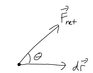
Now suppose that we’re interested in what is happening to our system during an infinitesmal time interval dt. We can multiply both sides by dt to find the equation dT = \vec{F}_{\textrm{net}} \cdot d\vec{r} \equiv dW_{\textrm{net}} where the right-hand side defines the infinitesmal work, dW. Let’s make a couple of useful observations about dW before we move on to integrating it, all of which apply to work in general. First of all, notice that dW is a scalar since it comes from a dot product. In fact, we can rewrite it using one of our dot-product identities as dW_{\textrm{net}} = F_{\textrm{net}} dr \cos \theta.
It’s important to emphasize a few special cases that can be counter-intuitive:
- dW_{\textrm{net}} can be zero, even if F_{\textrm{net}} is non-zero. (From above, this happens when \theta = 90^\circ, i.e. when \vec{F}_{\textrm{net}} is perpendicular to dr.)
- dW_{\textrm{net}} can be negative, if F_{\textrm{net}} and d\vec{r} point in opposite directions. (A simple example is a particle which is decelerating, so the net force is opposite its direction of motion.)
If we integrate both sides as our mass moves from point \vec{r}_1 to point \vec{r}_2, then we find the result T_2 - T_1 = \int_{\vec{r}_1}^{\vec{r}_2}\ dW_{\textrm{net}} = \int_{\vec{r}_1}^{\vec{r}_2}\ d\vec{r} \cdot \vec{F}_{\textrm{net}}, or more compactly, if we call the result of the integral over dW_{\textrm{net}} as just W_{\textrm{net}} (the net work), then we find:
The change in kinetic energy of a point mass as it moves from \vec{r}_1 to \vec{r}_2 is equal to the net work done:
\Delta T = W_{\textrm{net}} \equiv \int_{\vec{r}_1}^{\vec{r}_2}\ d\vec{r} \cdot \vec{F}_{\textrm{net}}.
This is an important relationship, because it gives us a way to interpret what kinetic energy actually means physically.
First, a brief comment on my notation above. It’s important to emphasize that the work-KE theorem is only true for a single point mass, and that it’s only true if we use the net force. However, it’s often useful to define the work done by a single force, which we can do using the same equation, W = \int_{\vec{r}_1}^{\vec{r}_2} d\vec{r} \cdot \vec{F}. Since d\vec{r} \cdot \vec{F}_{\textrm{net}} splits apart into d\vec{r} \cdot \vec{F}_1+ d\vec{r} \cdot \vec{F}_2 + ... in the case of multiple forces, the work also splits apart neatly, W_{\textrm{net}} = W_1 + W_2 + ....
Before we get to solving specific problems, the “big picture” we can see from the work-KE theorem is that changes in kinetic energy tell us something about the overall motion of a physical object. Although we can calculate T for an object at any moment in time, the significance of T is that it summarizes the history of how our object has moved. If our object starts from rest, the value of T later on is related to the sum total of all of the net forces acting in the direction of its path.
We’ll get to how to deal with the integral shortly, but there’s a specific case where it’s easy to simplify. If the net force is constant, then W = \vec{F}_{\textrm{const}} \cdot \int_{x_1}^{x_2} dx = \vec{F}_{\textrm{const}}\ \cdot \Delta \vec{x} which will be useful for considering some simple examples.
Here, you should complete Tutorial 4A on “Work-KE theorem”. (Tutorials are not included with these lecture notes; if you’re in the class, you will find them on Canvas.)
You drop your phone (mass m = 200 g) on the floor, from a height of 1m and from rest; fortunately, it’s in a protective case so it isn’t broken! But you notice a 0.5mm dent left in the case. Assuming that the floor provided a constant force F to stop your phone’s fall, how large is F in Newtons?
Answer:
First, we want to know how fast the phone is moving when it gets to the ground, which is a simple kinematic formula: first, the time to hit the ground is h = \frac{1}{2} gt_f^2 \Rightarrow t = \sqrt{\frac{2h}{g}} = 0.45\ \textrm{s} and then the speed at this time is v_f = v(t_f) = gt_f = 4.4\ \textrm{m}/\textrm{s}.
Now we’re almost done, since the last step is to apply the work-KE theorem. With a constant force, the work is just W = Fd, where d is the stopping distance of 0.5 mm (the size of the dent.) Setting this equal to the change in KE, we have F d = \frac{1}{2} mv_f^2 - 0 \Rightarrow F = \frac{1}{2d} mv_f^2. Plugging in numbers, we have a force of 650 N, which would give an acceleration of about 330 times g - pretty substantial, but not necessarily enough to break the phone, fortunately!
4.1.1 Line integrals
Before we can continue our study of work and kinetic energy, we have to deal with an important question: how do we evaluate the integral for work in general? Having another look at it: W_{\textrm{net}} = \int_{\vec{r}_1}^{\vec{r}_2} \vec{F}_{\textrm{net}} \cdot d\vec{r} How do we interpret this integral, where the integration variable is a vector? The best way to understand what this expression means is to go back to the infinitesmal picture for dW, and imagine building up the whole integral by just stringing together infinitesmal pieces:
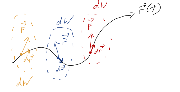
So the integral for W is a sum along the path traced out by \vec{r}., W = \sum_i dW_i \rightarrow \int dW
where the sum becomes an integral as we make our steps along the trajectory d\vec{r} smaller and smaller. Notice that this is not the “area under the curve” or anything related to it; we’re summing up the dot products \vec{F}_{\textrm{net}} \cdot d\vec{r} as we follow the curve. This is an example of a line integral.
There’s one special case where we already know how to do the integral: if the motion is one-dimensional. For one-dimensional motion, all vectors have only one component, so the dot product is trivial. If we call our single direction x, then W_{1d} = \int_{x_1}^{x_2} \vec{F}_{\textrm{net}}(x) \cdot d\vec{x} (I’m keeping the dot product notation to remind us that the directions still matter in one dimension, so we can get minus signs here.)
Now let’s pick a concrete example in two dimensions to see how things get tricky. Suppose that we have a constant force of the form \vec{F} = Fx\hat{x} + 2F\hat{y}, and we’d like to compute the work from \vec{r}_1 = (0,0) to \vec{r}_2 = (2,1).
First question: how do we interpret the vector differential d\vec{r}? We already know that derivatives of vectors are simple to evaluate: we just take the derivative of each component. Similarly, d\vec{r} just means we have a differential length in each component. In Cartesian coordinates, d\vec{r} = dx \hat{x} + dy \hat{y} + dz \hat{z}. So in our example, we can evaluate the dot product to find W = \int_{\vec{r}_1}^{\vec{r}_2} (Fx dx + 2F dy). The appearance of two differentials at once, dx and dy, signals that we can’t just evaluate this integral normally yet. More importantly, we have to specify one more thing not written down, which is the path along which we want to evaluate this integral. This is one of the sloppy things about this notation, although it’s used commonly: there are infinitely many ways to get from \vec{r}_1 to \vec{r}_2!
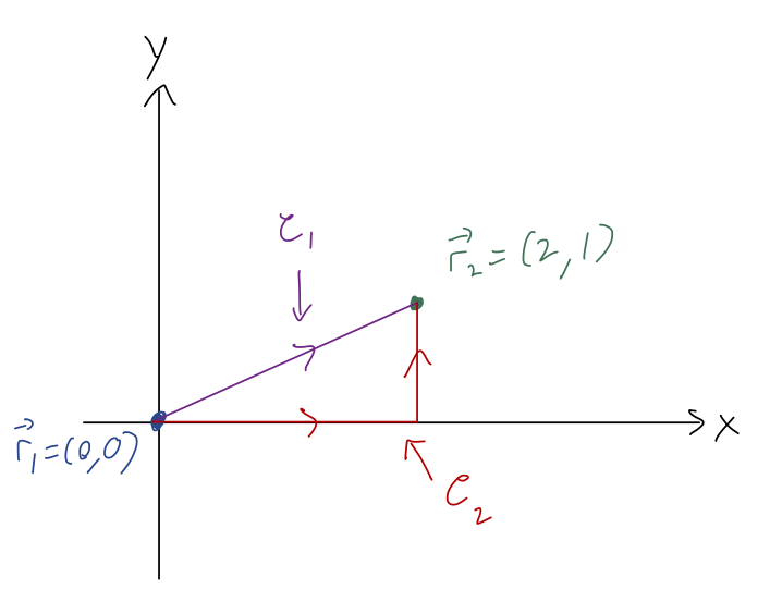
When we do a line integral, we’re actually choosing a directed path, hence the arrows on the sketch above, which tell us where we start and where we end. Just like a regular integral, if we go backwards (reverse the limits of integration so we move from \vec{r}_2 to \vec{r}_1), then we get an extra minus sign.
In math books, the integral will often be written instead as W = \int_{\mathcal{C}} \vec{F} \cdot d\vec{r}, where \mathcal{C} denotes a curve - the entire path we take, along with its endpoints. In physics applications, when we do the work integral, the curve is often just \vec{r}(t), the trajectory followed by our point mass.
Let’s pick one of the curves above and try to evaluate the integral. I’ll start with the straight line path, \mathcal{C}_1. If we think about it for a moment, the way a path is mathematically defined is an equation relating our coordinates to each other. In this case, we can write simply y = \frac{1}{2}x along \mathcal{C}_1. This relationship is true as long as we follow the curve. But we can use this to collapse our two differentials together: we have dx = 2dy so we can rewrite the line integral as W_1 = \int_{\mathcal{C}_1} (F xdx + 2F dy) \\ = \int_0^1 (F (2y) (2 dy) + 2F dy) \\ = F \left( \left. 4 \frac{y^2}{2} \right|_0^1 + \left. 2y \right|_0^1 \right) \\ = 4F.
This shows the basic idea of evaluating a line integral: although it looks like it has multiple coordinate differentials in it, when we move along a specific line, we can relate our coordinates together and collapse down to a single differential. Then we just have a normal integral to do! (It will always be a single integral, because a line is one-dimensional; we can always describe the distance along a line using a single number, whether the line is curved or not.)
An important feature of this method is that the way in which we collapse our multiple coordinates down to one is not unique. For example, we could have replaced dy instead of dx, and we’ll get the same answer: W_1 = \int_{\mathcal{C}_1} (Fx dx + 2F (dx/2)) \\ = \int_0^2\ F(1+x) dx \\ = F \left. x \right|_0^2 + F \left. \frac{1}{2} x^2 \right|_0^2 \\ = 4F. We don’t even have to stick to x and y! Another way to describe \mathcal{C}_1 is using a parametric equation: if we call our parameter s, then x(s) = 2s \\ y(s) = s \\ also defines the line y=x/2; try plugging in x(s) and y(s) to the line equation if it’s not obvious! Looking at the endpoints, we start at s=0 and end at s=1. Now we replace both coordinates, using dx = 2ds and dy = ds: W_1 = \int_{\mathcal{C}_1} (F (2s) (2 ds) + 2F ds) \\ = \int_0^1\ 2F (2s+1) ds = 4F.
Any line integral is always, implicitly, an integral against some single parameter s that describes the curve \mathcal{C} we are integrating along. Sometimes, it’s convenient to use coordinates like x or y as the parameter s, but we don’t have to. Pick whatever s is most convenient for a given curve!
Here’s yet another parameterization of the same curve: x(u) = 1-u\\ y(u) = (1-u)/2 where u runs from +1 to -1. Verify that this gives the same answer as above!
Answer:
First, we have to convert the differentials: from above we see dx = -du and dy = -du/2. Then we can plug in to the integral:
W_1 = \int_{\mathcal{C}_1} (F (1-u) (-du) + 2F (-du/2)) \\ = \int_{+1}^{-1} du\ F (-1 + u - 1) \\ = \left. F (-2u + \frac{1}{2}u^2) \right|_{+1}^{-1} = 4F.
No matter how we parameterize the curve, the result will always be the same - we’re not changing anything except how we choose to describe it. Finding a good parameterization can be kind of an art (like choosing a good set of coordinates!) In physics applications, time itself is often a good parameter to describe the path - we’re already used to solving for the motion \vec{r}(t)!
Now let’s consider the second curve \mathcal{C}_2. This is, in general, a different integral - even though the endpoints are the same, the path is different! This path isn’t a smooth curve - it has a sharp corner where the path suddenly changes. This means that we should do the integral piecewise, meaning that we divide up the path into smooth parts and deal with them one at a time. Here, the pieces of the path are very simple: from the origin, we have the curve y = 0 (which also implies dy = 0). For the second path of the curve, we have the fixed value x=2 - since this is constant, we see also that dx = 0. Thus, we can write the work integral along \mathcal{C}_2 as: W_2 = \int_{\mathcal{C}_2} (F x dx + 2F dy) \\ = \int_0^2 F x dx + \int_0^1 2F dy \\ = 2F + 2F = 4F.
In this particular case, we got the same answer again! In fact, this is not just a coincidence: you will get 4F for any path from (0,0) to (2,1) and this particular force. There is a deeper reason for this that we will see soon - but keep in mind, this is NOT guaranteed to be true for any force, so don’t just assume you can pick any path for an arbitrary force!
By the way, it’s often useful to visualize what’s going on in these line integrals before we just do the math out. Sketching the paths is only half of the visualization, because the direction and size of the force also matters. However, while the path is just a single line through space, the force \vec{F} is generally defined everywhere in space. As a result, we visualize it by drawing a force field plot. (A vector field is just a set of vectors that exist everywhere in space, whose values and directions are functions of position.)
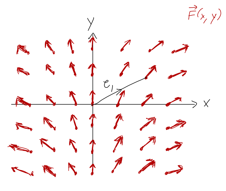
This makes it simpler to understand the work resulting from certain paths. In particular, if we move perpendicular to the force field, then \vec{F} \cdot d\vec{r} is always zero and the work will be zero. For path \mathcal{C}_1 (or \mathcal{C}_2 as well), we can easily predict from the force field plot that the work will be positive, since we are generally moving in the same direction that the force points (so \vec{F} \cdot d\vec{r} > 0.)
Since it’s often useful to sketch vector fields, it’s worth knowing that Mathematica has a function to do it for us, the VectorPlot[] function. Here’s an example:
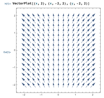
In Mathematica, vectors are denoted using curly braces {,}. You can see the input notation for VectorPlot above: the first argument is the vector field as a function, i.e. we enter {F_x, F_y} = {x, 2} for the vector field we’ve been working with. The last two arguments define the variable names and range to plot over, first x and then y.
Here, you should complete Tutorial 4B on “Line integrals”. (Tutorials are not included with these lecture notes; if you’re in the class, you will find them on Canvas.)
4.1.2 Line integrals and curvilinear coordinates
There are certain forces and/or certain paths for which the other coordinate systems we introduced this semester (cylindrical and spherical) will make things a lot simpler. For paths, working in different coordinates just gives us to a different way to parametrize the path - if we have a circular path, for example, then polar coordinates might be helpful. But as we’ve seen, there are usually multiple ways to choose the parameter s for any given path.
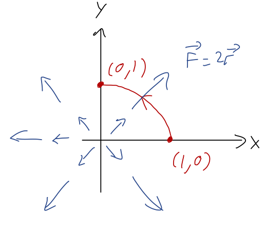
On the other hand, curvilinear vector coordinates can be very powerful for simplying line integrals whenever the force is most easily written using cylindrical or spherical components. To see this, let’s do another example. Suppose we have a force which is proportional to the polar unit vector \hat{\phi}, \vec{F} = F\hat{\phi} and we’re interested in the work done along a counterclockwise half-circle path from (1,0) to (-1,0).
Sketching vector fields makes my hand hurt, so here’s another Mathematica plot:
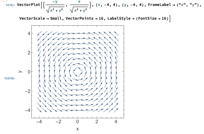
(I converted from polar to Cartesian for the plot - more on that below.) Think about it - does this match what you expected the plot to look like?
Next, we need d\vec{r} so we can find the dot product. Since we have \vec{F} in polar coordinates, we should use d\vec{r} in the same coordinates. We’ll assume z=0, but in full 3-d cylindrical coordinates, we know that \vec{r} = \rho \hat{\rho} + z \hat{z} To find d\vec{r}, one way would just be to start with the Cartesian version d\vec{r} = dx\ \hat{x} + dy\ \hat{y} + dz\ \hat{z} and apply our coordinate change. More directly, we can just calculate the derivative of \vec{r} with respect to some parameter, like t, and then cancel off the dt’s. Let’s try it that way: \frac{d\vec{r}}{dt} = \dot{\rho} \hat{\rho} + \rho \frac{d\hat{\rho}}{dt} + \dot{z} \hat{z} \\ = \frac{d\rho}{dt} \hat{\rho} + \rho \frac{d\phi}{dt} \hat{\phi} + \frac{dz}{dt} \hat{z} using the result for d\hat{\rho}/dt that we worked out back at the start of the semester. Cancelling off the dt’s, d\vec{r} = d\rho\ \hat{\rho} + \rho d\phi\ \hat{\phi} + dz\ \hat{z}. In case you ever need it, I’ll save you some trouble and give you the result for spherical coordinates: d\vec{r} = dr\ \hat{r} + r d\theta\ \hat{\theta} + r\sin \theta d\phi\ \hat{\phi}.
Using our result, we have the simple result dW = \vec{F} \cdot d\vec{r} = F \rho d\phi
Next, we parameterize the half-circular path. Any time we have a path like a circle or a spiral, an angle is a natural parameter to use. In fact, since this is just a section of the unit circle, we can easily write the path in the trivial-looking form \rho = 1, \\ \phi = \phi, starting at \phi=0 and ending at \phi=\pi. Thus, the integral can be written simply as W = \int_0^\pi F d\phi = \pi F. (Don’t be confused by units! Remember, our path has units of distance, so this is something like “pi meters times the constant force F.”)
Note that the length of the path can also be found by a line integral, which amounts to adding up a bunch of infinitesmal length segments: \ell = \int |d\vec{r}| = \int \sqrt{d\vec{r} \cdot d\vec{r}} = \int \sqrt{\rho^2 d\phi^2} = \int_0^\pi \rho\ d\phi = \pi (this is also easy to find geometrically as just half the circumference of a circle, of course.) So in this case, just like in our one-dimensional examples, we have simply W = F \ell. This happens because for this particular path and force, \vec{F} and d\vec{r} point in the same direction as one another along the entire path.
In this problem it was sort of obvious to choose polar coordinates, because of how we were given the force. But we could have been given \vec{F} in Cartesian coordinates instead: \vec{F} = -\frac{y}{\sqrt{x^2 + y^2}} \hat{x} + \frac{x}{\sqrt{x^2 + y^2}} \hat{y} You might be able to spot the fact that this is just \hat{\phi} from the expression, but a more reliable way to see that polar coordinates might be the way to go would be to plot the force field (this is one reason plotting vector fields is useful!) If you didn’t spot it, your integrals would be a lot more painful…
Another important note on coordinate dependence: it’s generally a better idea to let the force field dictate the coordinate choice, rather than the path. For example, suppose we had this same circular force, but the straight-line path y = x/2 from our previous example. It’s actually not so hard to parametrize that path in polar coordinates: remembering how polar and Cartesian are related, the line equation above becomes \rho \sin \phi = \frac{1}{2} \rho \cos \phi \Rightarrow \tan \phi = \frac{1}{2}. So this is a path with constant \phi and constant z, giving d\vec{r} = d\rho \hat{\rho}. We don’t have to go any further, since \vec{F} \cdot d\vec{r} = 0 and the work is just zero. (It will still be zero in Cartesian coordinates, but the integral will be much more work!)
That was too easy, since a straight line through the origin is just in the \hat{\rho} direction and therefore still nice in cylindrical coordinates. What about this path, the fixed vertical line x=1 from (1,1) to (1,-1)?
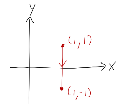
The equation for this line in polar coordinates is x = 1, which is just \rho = 1 / \cos \phi. This path changes in both \rho and \phi, so in general we will pick up both; but for the force we’re considering \vec{F} = F \hat{\phi}, the dot product is still \vec{F} \cdot d\vec{r} = \rho d\phi. Thus, the work integral still takes the same form we found above, W = \int \vec{F} \cdot d\vec{r} = \int F \rho d\phi \\ = F \int_{\pi/4}^{-\pi/4} \frac{d\phi}{\cos \phi} \\ \approx (-1.76\ {\textrm{m}}) F where I used Mathematica to do the integral numerically - it ends up being a complicated combination of logs and trig functions. I’m just reading the \phi limits of integration off the plot geometrically, but in general we get them by solving the equation of our line at the given points.
Here’s a more interesting line, y = 1 + x/2 from (0,1) to (2,2):
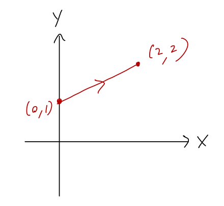
What is the line integral \int_{\mathcal{C}} \vec{F} \cdot d\vec{r} over this curve, for the force \vec{F} = F\hat{\phi}?
Answer:
If we substitute in the coordinate conversions for both x and y in polar, the equation for the line becomes: \rho \sin \phi = 1 + \frac{1}{2} \rho \cos \phi \\ \rho (2\sin \phi - \cos \phi) = 2 \\ \rho(\phi) = \frac{2}{2\sin \phi - \cos \phi}. How about the endpoints? At (0,1) we obviously have \phi = \pi/2; plugging this in to our \rho(\phi) is a good check of our work, and it gives \rho(\pi/2) = \frac{2}{2 - 0} = 1 which is correct. The other endpoint is at \phi = \pi/4, so our line integral is (using \vec{F} \cdot d\vec{r} = F \rho d\phi from above): W = \int_{\pi/2}^{\pi/4} d\phi \frac{2}{2\sin \phi - \cos \phi} d\phi I wouldn’t want to do this integral by hand, although it does have a closed-form answer in terms of \tan and \tanh. Doing it numerically, I find W \approx (-1.2\ \textrm{m}) F.The moral of these examples is that the force is the most important factor in your choice of coordinate system for a line integral, because we have to deal with the vector components of the force. Once that’s out of the way, it’s easy to make our path conform to whatever coordinates we’ve chosen.
To recap, when faced with a line integral, we need to work through the following steps to find the answer:
- Choose vector coordinates and find \vec{F} \cdot d\vec{r}. (The form of \vec{F} is usually most important in coordinate choice, but don’t ignore the path completely.)
- Parameterize the path, writing it in terms of a single coordinate or parameter.
- Use the results of 1) and 2) to write the work integral as a regular integral over our single parameter.
- Do the integral and find the answer!
If you feel like you need more line integral practice, here’s one more exercise you can try.
Calculate the work integral W = \vec{F} \cdot d\vec{r} for the force \vec{F} = 2\vec{r} and parabolic path x = 1-y^2, from (1,0) to (0,1).
Answer:
Let’s start by sketching the path:
It might be tempting to choose polar coordinates since the force field is radial, but radial force is pretty easy to describe in Cartesian coordinates too, and our path will be easier in Cartesian. (If we had a force in the \hat{\phi} direction, we’d almost certainly want polar instead!) Using Cartesian, we have \vec{F} = 2x \hat{x} + 2y \hat{y} and so \vec{F} \cdot d\vec{r} = 2Fx dx + 2Fy dy.
Next, we parameterize the path. Here y itself is a nice parameter, since we already have the path written in the form x = 1-y^2. In terms of differentials, we have dx = -2y dy and in terms of y, our path begins at y=1 and ends at y=0. So writing out our line integral, W = \int \vec{F} \cdot d\vec{r} = \int (2Fx dx + 2Fy dy) \\ = 2F \int_1^0 (1-y^2) (-2y dy) + y dy \\ = 2F \int_1^0 dy\ (-y + 2y^3) \\ = 2F \left. \left(-\frac{y^2}{2} + \frac{y^4}{2} \right) \right|_0^1 \\ = 0.
Although the work is exactly zero here, it’s sort of a coincidence: we notice that the cancellation of y^2 and y^4 only worked at y=0 and y=1, so pretty much any other starting or ending points along this curve would yield non-zero work.
4.2 Potential energy
Now that we know how to calculate line integrals, let’s go back to the physical meaning of work. In mechanics, we aren’t going to be dealing with completely arbitrary paths; the work-KE theorem only applies to the path which results from Newton’s laws and whatever forces are applied.
At the beginning of this section, I mentioned that energy comes in many forms. To really see how work and energy can be useful, we need to introduce a second form of energy, which is called potential energy. You may remember the buzzwords from intro physics: a potential energy can only be defined for a conservative force. This turns out to be a consequence of how we define a conservative force, acting on a point mass:
- Conservative forces depend only on \vec{r} and constants.
- The work done by a conservative force from \vec{r}_1 to \vec{r}_2 is independent of the path taken.
When both of these properties are satisfied, if we’re given two points anywhere in space, we immediately know the work done by the conservative force when we move from one to the other. (Property 1 matters because we don’t need any extra info to decide the work done, like how long it took to move between the points or how fast the object was moving.)
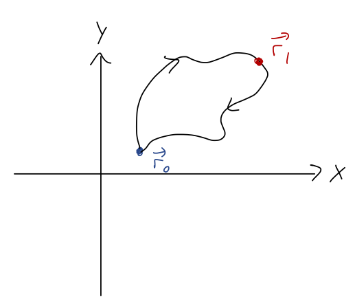
Now let’s pick a special point \vec{r}_0 somewhere in space and hold it fixed. The work done to get to any other point \vec{r} from this special point is a function only of where the second point is: W_{\vec{r}_0 \rightarrow \vec{r}} = \int_{\vec{r}_0}^{\vec{r}} \vec{F} \cdot d\vec{r} = -U(\vec{r}) This defines the potential energy function. (It only depends on \vec{r}, because we’ve agreed to hold \vec{r}_0 fixed.) The minus sign I added at the end is extremely important, as we’ll see below! Basically, it has to do with energy conservation: positive work will give a positive change in kinetic energy, which will be compensated by a negative change in potential energy so the total stays fixed.
Now, let’s do a short mathematical proof that will let us make two nice observations. If we try to calculate U(\vec{r}_0), we find the following: U(\vec{r}_0) = -\int_{\vec{r}_0}^{\vec{r}_0} \vec{F} \cdot d\vec{r} \\ = -\int_{\vec{r}_0}^{\vec{r}_1} \vec{F} \cdot d\vec{r} - \int_{\vec{r}_1}^{\vec{r}_0} \vec{F} \cdot d\vec{r} where I’m now just picking another arbitrary point \vec{r}_1 and using the properties of definite integration to split it up. Okay, this isn’t a normal integral. Really, the original line integral represents a closed path from \vec{r}_0 back to itself, and I’ve picked a point somewhere along that path and divided it in half:
Reversing the limits of any integral, including a line integral, just gives us a minus sign: U(\vec{r}_0) = -\int_{\vec{r}_0}^{\vec{r}_1} \vec{F} \cdot d\vec{r} + \int_{\vec{r}_0}^{\vec{r}_1} \vec{F} \cdot d\vec{r} = 0. These two integrals are on two different curves, but since \vec{F} is conservative it doesn’t matter; their results are equal and they cancel. The first nice observation is that picking a reference point is the same thing as choosing where our potential energy function is equal to zero, which you’ll remember as something you can do with e.g. the gravitational potential.
If you choose a different reference point \vec{r}'_0, then your potential energy function will be different, but in a simple way: U'(\vec{r}) = -\int_{\vec{r}'_0}^{\vec{r}} dW = -\int_{\vec{r}'_0}^{\vec{r}_0} dW - \int_{\vec{r}_0}^{\vec{r}} dW \\ = U(\vec{r}_0') - U(\vec{r}) or in other words, the difference between U and U' is just a shift by a constant.
The second nice observation we can make is that we’ve just showed that for any force which satisfies property 2 above (work done is path-independent), the work done around a closed path is exactly zero. You may remember the special notation for closed-path integrals from vector calculus: \oint \vec{F} \cdot d\vec{r} = 0. If you remember that notation, you probably also remember that \vec{F} \cdot d\vec{r} shows up in a very powerful result called Stokes’ theorem. We’ll come back to that later on: it will give us a much clearer picture of why any particular force should obey property 2 above, which seems sort of arbitrary right now.
Back to our general discussion of potential energy U. Assuming for the moment that the corresponding \vec{F} is the only force acting, the work-KE theorem applies: T(\vec{r}_2) - T(\vec{r}_1) = W_{1 \rightarrow 2} = \int_{\vec{r}_1}^{\vec{r}_2} \vec{F} \cdot d\vec{r} = -U(\vec{r}_2) + U(\vec{r}_1) or rearranging, T(\vec{r}_1) + U(\vec{r}_1) = T(\vec{r}_2) + U(\vec{r}_2). In other words, the combination E = T + U, which we call the mechanical energy (or just “the energy” when we’re doing classical mechanics), doesn’t change as we move from \vec{r}_1 to \vec{r}_2. Since this is true for any two points we choose, and since the path and other variables can’t change the work, we see that in the presence of a conservative force, energy is conserved: \frac{dE}{dt} = 0.
Since we used the work-KE theorem, we technically assumed above that \vec{F} is the only force acting in our system. If we have multiple forces, remember that we can divide net work up into the sum of work due to each individual forces. If they’re all conservative, then we can write a separate potential energy function for each force. So the more general version of the mechanical energy is E = T + U_1 + U_2 + U_3 + ... if we have several forces \vec{F}_1, \vec{F}_2, \vec{F}_3...
Of course, as we just noted there are plenty of non-conservative forces around. The work-KE theorem still applies to them, and we can still split them up. If we have both conservative and non-conservative forces, then \Delta T = W_{\textrm{net}} = W_{\textrm{cons}} + W_{\textrm{non-cons}} \\ = -\Delta U + W_{\textrm{non-cons}} or \Delta E = W_{\textrm{non-cons}} So energy is not conserved if we have non-conservative forces, but we know exactly how it will change if we keep track of the work done by those forces.
Here’s a quick note about the deeper interpretation of this absence of energy conservation, since I commented early that conservation of energy is a really important and general physical principle. Friction and air resistance are not fundamental forces: ultimately, they come from electromagnetic forces between the atoms in our object and the surface or medium providing the force. All of the known fundamental forces of nature are conservative, which means that total energy is conserved, period. When we find a non-zero \Delta E due to something like friction, that “lost” energy is just being transferred into another form - mostly heat, in the case of friction. When multiple conservative forces are present, energy will be exchanged between the different potentials and kinetic energy (see here for a classic example!), but total E is always the same.
One more brief aside, about magnetic fields, which are sort of a weird example. They are non-conservative because they depend on speed, but they also don’t do any work at all because the magnetic force is always perpendicular to \vec{v}! So a system including a magnetic field will still conserve mechanical energy - but we can’t write a potential energy function (of the form we’re using here) to describe the motion. (In other words, conserving energy alone isn’t sufficient for a force to be “conservative” by the definition we’re using.) Normal forces are even weirder, but they fall into the same category as magnetic force: they usually don’t do any work at all, but they’re not technically considered to be conservative and we can’t use potential energy to describe normal forces.
At this point, Taylor does an example of mixing conservative and non-conservative forces, involving a sliding block with friction. We solved the sliding block with friction way back in chapter 1, but work gives a quicker way to find the speed as a function of the height of the block. I’ll skip this example because Taylor already did it, and unfortunately there aren’t any other good simple examples of this sort of thing: you could try to do a similar trick with linear air resistance, but the equations are unsolvable and you have to resort to numerics anyway, so using energy and work doesn’t really help.
Let’s do a concrete example: a charge +q is suspended in a uniform electric field, \vec{E} = E_0 \hat{x}. The force on the charge is proportional to the field \vec{F} = q\vec{E} = qE_0 \hat{x}.
The force due to a (static) electric field is conservative, so we can go ahead and calculate a potential energy function by using the definition: U(\vec{r}) = -\int_{\vec{r}_0}^{\vec{r}} \vec{F} \cdot d\vec{r} = -\int_{\vec{r}_0}^{\vec{r}} qE_0 dx.
Normally, to continue we’d need to pick a reference point \vec{r}_0 and a path to integrate along - even if we know the answer will be path-independent, we have to choose one! However, in this case since the force is constant, we can see that the path doesn’t matter at all: the result of the integral is U(\vec{r}) = -qE_0 (x - x_0) or simply U(x) = -qE_0 x if we pick \vec{r}_0 to be the origin (0,0,0), which is clearly the simplest choice. This is a rare example where we can immediately tell that a force is conservative just by trying to calculate the work.
Let’s think briefly about the answer: we see that since U(x) \sim -x, the potential decreases as x increases. This makes sense, since the electric field will push our charge in the +\hat{x} direction; as it moves it will pick up kinetic energy (\Delta T > 0), so energy conservation requires that it lose an equal amount of potential energy (\Delta U < 0.) This should remind you of what you already know about gravitational potential U(z) = +mgz near the Earth’s surface.
Let’s go back to the example force that we were looking at to start our discussion of line integrals, \vec{F} = Fx\hat{x} + 2F\hat{y}.
I mentioned in passing that it wasn’t a coincidence that we kept finding the same answer for different paths with this force - it is, in fact, conservative. So let’s find the potential energy function: U(\vec{r}) = -\int_{\vec{r}_0}^{\vec{r}} \vec{F} \cdot d\vec{r} = -\int_{\vec{r}_0}^{\vec{r}} Fx' dx' + 2F dy'.
(I’m using primed coordinates under the integral to avoid some confusion.) For simplicity, let’s take \vec{r}_0 to be the origin again. In order to do this integral and find U(\vec{r}), this time we will need to pick a path. Vector field plots are always a useful place to start when deciding on a path! Here’s the field plot for this force field once again:
This is a little abstract, since our path has to be valid for any choice of x and y, but any sufficiently general curve will do. For example, we can take a straight-line path, but if we do that we have to let the slope be variable. Letting y' = bx', we have dy' = b dx', which we can use to simplify down the integral:
U(\vec{r}) = -\int_0^{x} Fx' dx + 2F (b dx') \\ = -\frac{1}{2} F x^2 - 2Fbx.
Now we have to deal with the slope b - we introduced that variable with our path choice, so we have to get rid of it. Remember that we’re finding the potential at a given point \vec{r} = (x,y,z). For the path to reach that point, we must also have y = bx, or b = y/x. Plugging back in gives us our answer: U(x,y) = -\frac{F}{2} (x^2 + 4y).
Just to make sure, let’s re-compute the answer using another path. In fact, although the straight-line path was simple to set up, it’s not really the simplest path we can use. Generally, moving along or perpendicular to field lines whenever possible will simplify our line integrals. Let’s do a piecewise path where we move along the y-axis first (so dx = 0), and then horizontally in the x direction (so dy = 0). This splits our answer into two integrals: U(\vec{r}) = -\int_0^y 2F dy' - \int_0^x Fx' dx' \\ = -2Fy - \frac{1}{2} F x^2
exactly as we found with the straight-line path, but now in just one step!
4.2.1 Force from the potential
Let’s come back to the relationship between potential energy and force. We defined the potential based on a path integral of the force: U(\vec{r}) = -\int_{\vec{r}_0}^{\vec{r}} \vec{F} \cdot d\vec{r}, which uses \vec{F} to find U. But we know that regular integrals can be inverted using derivatives, so it’s natural to ask: can we go the other way here as well, i.e. can we find \vec{F}(\vec{r}) given U(\vec{r})?
The answer is yes, and the easiest way to see it is thinking about the infinitesmal version of the integral above. Remember that a line integral is just a sum over lots of infinitesmal segments, which means that we can go backwards and notice that an infinitesmal contribution to the potential energy takes the form dU = -\vec{F} \cdot d\vec{r} (you can think of this as the change in potential if we move \vec{r} by a tiny amount; also, we get the formula above back by integrating both sides.) There’s another way to write out dU(\vec{r}); by using the chain rule with respect to the individual coordinates, we have dU = \frac{\partial U}{\partial x} dx + \frac{\partial U}{\partial y} dy + \frac{\partial U}{\partial z} dz. We can write out the first version of dU in a very similar way by expanding the dot product: dU = -F_x dx - F_y dy - F_z dz These equations are both dU, so their right-hand sides have to be equal. But more than that, they have to be equal for any possible path that we choose! Changing a path will change how dx, dy, and dz vary, which means that for these equations to always be true, the things multiplying dx, dy, and dz must be equal. This gives us the result \vec{F} = -\frac{\partial U}{\partial x} \hat{x} - \frac{\partial U}{\partial y} \hat{y} - \frac{\partial U}{\partial z} \hat{z} or written more compactly, \vec{F} = -\vec{\nabla} U where \vec{\nabla} represents the gradient of the function U. (The upside-down triangle symbol is usually called ‘del’, although another common name is ‘nabla’, which comes from the Greek word for ‘harp’.) The gradient can be thought of as being defined through the equation \vec{\nabla} \equiv \frac{\partial}{\partial x} \hat{x} + \frac{\partial}{\partial y} \hat{y} + \frac{\partial}{\partial z} \hat{z} in Cartesian coordinates. Clearly from the way we found it, \vec{\nabla} acts as the inverse operation to a regular line integral, just as an ordinary derivative is the inverse of an ordinary integral. (Because it is a vector, \vec{\nabla} will look different if we change coordinates! I won’t go through those formulas for now, just warn you that it will happen.)
If you have more of a formal math background, you might recognize \vec{\nabla} as a sort of object called an operator. An operator is basically a map from one class of objects to another. In this case, it takes us from a scalar function U(x,y,z) to a vector function \vec{F}(x,y,z). You probably remember the two other common vector differential operators: the divergence (\vec{\nabla} \cdot), which takes a vector to a scalar, and the curl (\vec{\nabla} \times), which takes a vector to another vector. We’ll see more of them soon! If you’ve seen something like d/dx written on its own, that’s also an example of an operator.
One simple but important note about \vec{\nabla} is that it can be distributed over sums, i.e. if we have two different potential functions, \vec{\nabla} (U_1 + U_2) = \vec{\nabla} U_1 + \vec{\nabla}U_2. (In math terms, this corresponds to \vec{\nabla} being a linear operator.) This means that if we have two separate forces acting on an object, and we know each of their potential functions, then the total potential is just the sum of the individual ones. We already pointed this out before, but now it’s clearly related to the fact that when we have multiple forces, we just add them as vectors.
Since this is a physics class, the most physical explanation for what \vec{\nabla} U means is (in my opinion) in terms of differentials, specifically the relation dU = \vec{\nabla} U \cdot d\vec{r}. In other words, if we sit at some point \vec{r} in space and then ask the question “how does U change if I move a tiny distance d\vec{r} in some direction?”, the answer is encoded in the gradient \vec{\nabla} U(\vec{r}), which contains all of the directional derivatives of U at that point.
The differential version also gives us some nice insights into the meaning of \vec{\nabla} U as a vector. Suppose we sit at a single point, so \vec{\nabla} U is fixed, and then try to vary d\vec{r}. We’ll find that the largest dot product, and thus the largest dU, occurs when d\vec{r} points in the \vec{\nabla} U direction. So \vec{\nabla} U points in the direction of the largest rate of change of U(\vec{r}).
We can also see that if \vec{\nabla} U = 0, then dU = 0 regardless of which direction we choose. So wherever \vec{\nabla} U = 0, the function U(\vec{r}) must be at a local extremum (maximum or minimum, or possibly a saddle point.)
One more extremely useful observation: going back to the general case where \vec{\nabla} U \neq 0, we can see that if we take d\vec{r} in the direction perpendicular to \vec{\nabla} U, then dU = 0. If we keep traveling in the direction perpendicular to \vec{\nabla} U, we will trace out a line along which U is constant. This line is known as an equipotential. In fact, for a given \vec{\nabla} U there is a whole plane of perpendicular vectors we can choose, which means that in three dimensions we actually have a two-dimensional equipotential surface along which U doesn’t change.
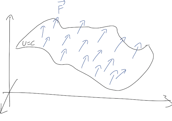
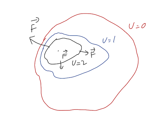
This gives us a useful way to visualize forces in two dimensions (the concept is still the same in three dimensions, but it’s very hard to draw!) Consider a point particle moving in the (x,y) plane, subject to some unknown force. In two dimensions, equipotential surfaces will just be lines, so we can make a contour plot showing the lines of constant U:
If you’ve ever read a topographic map, which shows lines of constant elevation in a top-down view, then you’re used to reading equipotential plots:
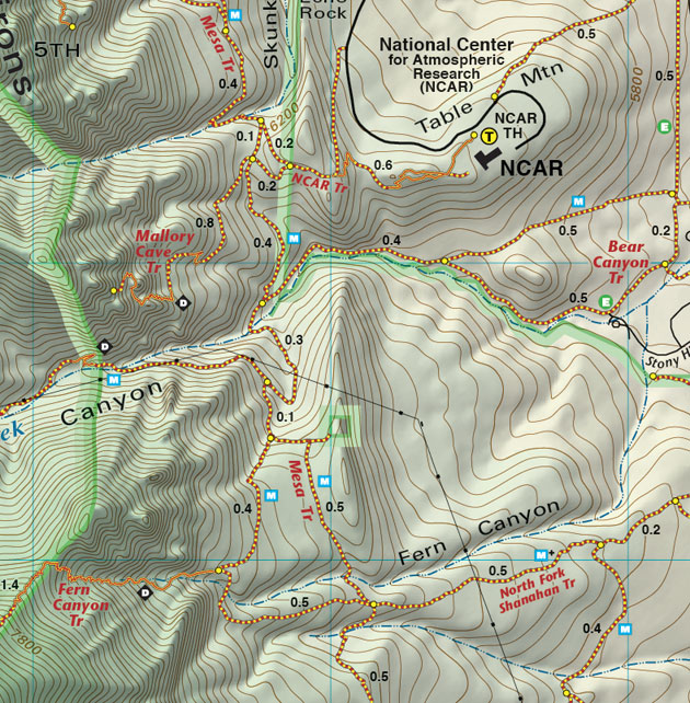
(source: https://www.latitude40maps.com/boulder-county-trails/)
Here the contours are equal height z, but since the gravitational potential U(z) \propto z, this is also a gravitational equipotential plot! This can give a useful metaphor for interpreting equipotential plots for other forces. In particular, it can help us remember the following facts:
- Equipotential lines never cross. This is basically true by definition: two different lines correspond to two different constant potential energies U_1 and U_2. Crossing would mean the potential can have two different values at the same point; our definition of a conservative force guarantees that can’t be true. For the topographic map, this is obvious - one point can’t have two heights!
- Force points “downhill”. In general, this means that since \vec{F} = - \vec{\nabla} U, the force is in the direction perpendicular to the equipotential lines and points towards smaller U. (In the topographic plot, this is literally downhill.)
- Spacing of lines tells us the magnitude of |\vec{\nabla} U|. Densely-spaced lines indicate that the potential is changing rapidly vs. position, indicating a large force. Again, this is intuitive for the topographic plot: lots of dense lines in a certain spot means a very steep slope.
Let’s gain some intuition by thinking about the details of equipotentials like this.
Here, you should complete Tutorial 4C on “Conservative Forces and Equipotential Diagrams”. (Tutorials are not included with these lecture notes; if you’re in the class, you will find them on Canvas.)
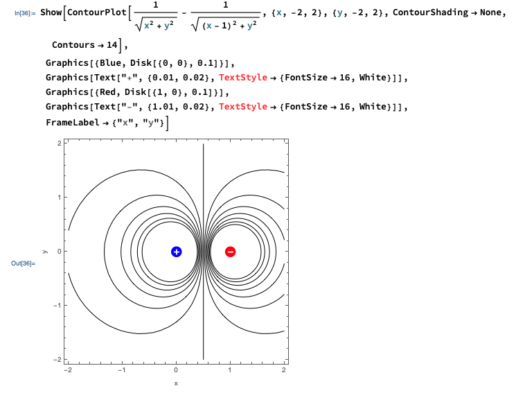
You won’t be surprised to learn that Mathematica has a function to make these plots for us, called ContourPlot[]. I won’t dwell on the details, but here’s a quick example showing how to make our own equipotential plot for a pair of electric charges.
Suppose a particle has a potential energy function of the form U(x,y,z) = 3x \cos(y/L) - 2z^2 (ignoring units for now, this is a math exercise.) What is the force?
Answer:
To find the force, we take the gradient: \vec{F} = -\vec{\nabla} U. For the gradient, we need to know the partial derivatives of U with respect to all three coordinates. We haven’t done any partial derivatives yet this semester, so let’s go through them: \frac{\partial U}{\partial x} = 3 \cos (y/L) \\ \frac{\partial U}{\partial y} = -\frac{3x}{L} \sin (y/L) \\ \frac{\partial U}{\partial z} = -4z (finding partial derivatives is easy: we just ignore everything that we’re not taking a derivative of.) Thus, the force is \vec{F} = -\vec{\nabla} U \\ = -\frac{\partial U}{\partial x} \hat{x} - \frac{\partial U}{\partial y} \hat{y} - \frac{\partial U}{\partial z} \hat{z} \\ = -3 \cos (y/L) \hat{x} + \frac{3x}{L} \sin (y/L) \hat{y} + 4z \hat{z}.
4.2.2 Curl and Stokes’ theorem
The operator \vec{\nabla} can be used to define other useful quantities, in addition to the gradient. One of these useful quantities is called the curl, where the curl of \vec{v} is denoted by \vec{\nabla} \times \vec{v}.
Before we do curl, let’s do a lightning review of the cross product. Unlike the dot product, the cross product \vec{a} \times \vec{b} gives us another vector instead of a number, and in particular \vec{a} \times \vec{b} by definition is perpendicular to both \vec{a} and \vec{b}. The magnitude of the cross product is |\vec{a} \times \vec{b}| = ab \sin \theta behaving in the opposite way to the dot product; in particular, notice that |\vec{a} \times \vec{a}| is always zero.
Now, given two different vectors \vec{a} and \vec{b}, there is a unique plane containing both of them; the direction of the cross product \vec{a} \times \vec{b} is then perpendicular to that plane. However, this isn’t quite enough information, because -\vec{a} \times \vec{b} is also perpendicular to the plane!
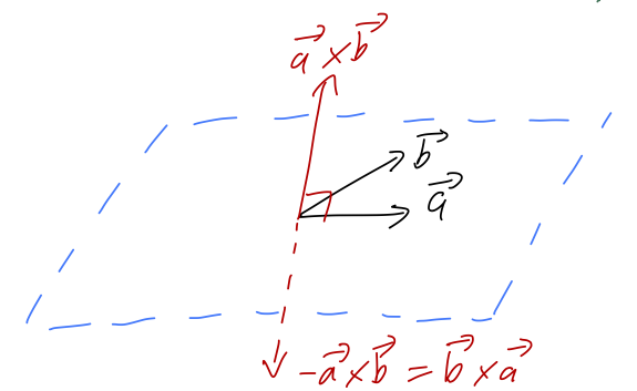
Deciding which of these two vectors to call the positive cross product is a choice of convention - which means it’s an arbitrary choice that we can make once, but then we have to keep that choice consistent. We will follow the standard physics convention, which is the right-hand rule: if you hold out your right hand with the thumb pointing in the direction of \vec{A} and your fingers in the direction of \vec{B}, then your palm points in the direction of \vec{A} \times \vec{B}. Try it with my diagram above!
The right-hand rule also fixes an ambiguity in our rectangular coordinates, which is that we could have picked either of these sets of axes:
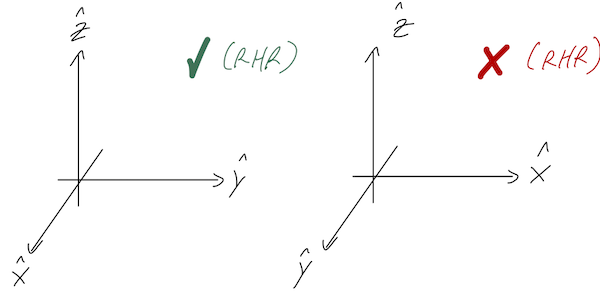
We always define our rectangular coordinates so that positive \hat{z} is a right-hand rule cross product of \hat{x} with \hat{y}. In other words, the directions of our rectangular unit vectors always satisfy: \hat{x} \times \hat{y} = \hat{z} \\ \hat{y} \times \hat{z} = \hat{x} \\ \hat{z} \times \hat{x} = \hat{y}. This is only one choice of convention, and not three; the first equation actually forces the other two to be true. An easy way to remember all three of these at once is to notice that they are all cyclic permutations: if you shift every vector to the left one spot, wrapping back around to the right at the left end, then you get the next formula.
There is a general, mechanical formula for the cross product in rectangular components, using a three-by-three matrix determinant: \vec{a} \times \vec{b} = \left|\begin{array}{ccc} \hat{x}&\hat{y}&\hat{z}\\ a_x&a_y&a_z\\ b_x&b_y&b_z\end{array}\right| \\ = (a_y b_z - a_z b_y) \hat{x} - (a_x b_z - a_z b_x) \hat{y} + (a_x b_y - a_y b_x) \hat{z}. We will use this a couple of times this semester, and you’ll see lots more of it next semester in classical mechanics 2.
Back to the curl. The cross product here is taken literally: the definition of curl is that we take the cross product of the gradient vector with the second vector. You’ll remember that one way to write the cross product is using a 3x3 determinant; using this notation here, the curl is (in Cartesian coordinates only!) \nabla \times \vec{v} = \left|\begin{array}{ccc} \hat{x}&\hat{y}&\hat{z}\\ \frac{\partial}{\partial x}&\frac{\partial}{\partial y}&\frac{\partial}{\partial z}\\ v_x&v_y&v_z\end{array}\right| \\ = \left( \frac{\partial v_z}{\partial y} - \frac{\partial v_y}{\partial z} \right) \hat{x} + \left( \frac{\partial v_x}{\partial z} - \frac{\partial v_z}{\partial x} \right) \hat{y} + \left( \frac{\partial v_y}{\partial x} - \frac{\partial v_x}{\partial y} \right) \hat{z}.
Now suppose we have a force \vec{F} which is conservative. By definition, that means we can find a potential function U so that \vec{F} = -\vec{\nabla} U. But now notice what happens when we try to take the curl of \vec{F} and write it in terms of U: (\vec{\nabla} \times \vec{F})_x = \frac{\partial F_z}{\partial y} - \frac{\partial F_y}{\partial z} \\ = \frac{\partial}{\partial y} \left( -\frac{\partial U}{\partial z} \right) - \frac{\partial}{\partial z} \left( -\frac{\partial U}{\partial y} \right). But the order of partial derivatives doesn’t matter: there’s only one \partial^2 U / \partial y \partial z, so both terms are the same. Therefore, (\vec{\nabla} \times \vec{F})_x = 0. Of course, we didn’t assume anything special about the x-direction, so it won’t surprise you to know that the whole curl is in fact zero! We’ve just proved the vector identity \vec{\nabla} \times \vec{\nabla} U = 0 for any function U. This means that if we have a conservative force, then its curl must be zero: \vec{\nabla} \times \vec{F} = 0.
Curl looks like kind of a weird and arbitrary quantity, so you might wonder why we care if a force has zero curl or not. The short answer is that this identity goes both ways: if we’re given a force \vec{F}, we can calculate its curl, and if it is equal to zero then the force must be conservative. So curl allows us to test for a conservative force!
This is a big deal, because you’ll remember that the second condition for a force to be conservative was that work done is independent of path, which is something you definitely can’t test directly - there are always an infinite number of paths. But we argued that the path-independence of work is equivalent to the condition that \oint \vec{F} \cdot d\vec{r} = 0, i.e. the work vanishes on any closed path (a path that goes back to the same point, i.e. a loop.) But now we come to an important vector calculus result, Stokes’ theorem, which I will state but not prove: \oint_{\partial \mathcal{S}} \vec{F} \cdot d\vec{r} = \int \hspace{-4mm} \int_{\mathcal{S}} (\vec{\nabla} \times \vec{F}) \cdot d\vec{A}
Those are some pretty dense symbols, so in words: “Consider a finite surface \mathcal{S}, with boundary curve \partial S. The surface integral of the curl of any vector over \mathcal{S} is equal to the line integral of the same vector around the boundary \partial S.”
We don’t need to go too deep into surface integrals for our current purposes; as the name implies, they are the two-dimensional equivalent of a line integral. The important point right now is that if we have a force for which the curl \vec{\nabla} \times \vec{F} vanishes, then its line integral around any closed loop anywhere is automatically zero by Stokes’ theorem.
We can get a little bit of intuition about this visually. We can consider taking our path over a given boundary curve \partial S, and drawing a bunch of small circular paths inside of S:
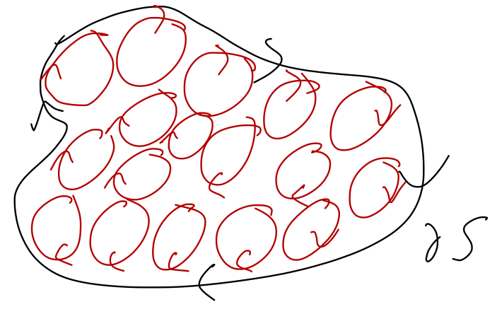
Around the perimeter, we can trace out a path along the edge of the circles which is close to the black path \partial S. In the interior of this region, the paths wherever two circles meet are running in the opposite direction. This means that if we add up the line integrals over all of the circles, we get (roughly) the line integral over the outer path \partial S!
Stokes’ theorem is precisely just the infinitesmal limit of this statement. If we fill the region with an infinite number of tiny circles, then the total path over all of them combined is exactly \partial S. What is the line integral over an infinitesmal circle? Well, if it’s really tiny, a square path will be about the same:
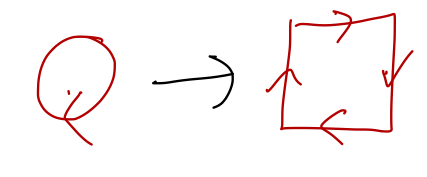
The two vertical paths give F_y(x,y) dy + F_y(x+dx,y) (-dy) = - \frac{\partial F_y}{\partial x} dx dy while for the two horizontal paths, we get similarly F_x(x,y) (-dx) + F_x(x,y+dy) (dx) = +\frac{\partial F_x}{\partial y} dx dy. Comparing back to our formula for the curl, this is exactly -(\nabla \times \vec{F}) \cdot (\hat{z} dx dy) = -(\nabla \times \vec{F}) \cdot d\vec{A} and integrating over the whole surface S to “add up” all of the infinitesmal circles gives us the right-hand side of Stokes’ theorem.
One more detail to deal with, that you might have already noticed: I have an extra minus sign on the curl of \vec{F} here, compared to how we wrote Stokes’ theorem above. Where did the sign come from? Did I make a mistake? In fact, I chose this path intentionally. Notice that if we reversed the path \partial S, we would get an extra minus sign. But there is a notational ambiguity in our original equation: when I write \oint_{\partial \mathcal{S}} \vec{F} \cdot d\vec{r}, does \partial \mathcal{S} mean the closed path the way I drew it (running clockwise), or the reversed path (counter-clockwise)? The answer should now be clear: when we write Stokes’ theorem without an extra minus sign, we mean the counter-clockwise path. This actually follows from the right-hand rule we saw above; if we adopted a left-hand rule for cross products, then the clockwise path would be positive \partial S instead.
In summary, there are several equivalent ways to state that a force \vec{F} is conservative:
- If the work done is path-independent;
- If \vec{F} = -\vec{\nabla} U for some function U;
- If \vec{\nabla} \times \vec{F} = 0 everywhere.
Curl is much more important in electrodynamics; in mechanics, it’s mostly important as a test for conservative forces. We’ll have more use for the divergence \vec{\nabla} \cdot \vec{F} later on, but for now let’s simply move on to our next topic.
4.3 Energy and one-dimensional systems
Although we’ve been working a lot in three dimensions with our vector calculus proofs, it turns out that some of the most powerful features of energy conservation arise in one-dimensional systems. It should be noted that “one-dimensional” here doesn’t mean “only moving along a line”; it refers to any physical system in which we only need a single coordinate to tell us the full state of the system.
A basketball in freefall with no horizontal motion is a one-dimensional system (we just need the height y), but so is a pendulum (just need the angle \theta), or even a roller coaster (it’s stuck on a track, so we can describe it in terms of s, the distance along the track.) For simplicity, we’ll call our single coordinate x in the following.
What about conservative forces? Taylor shows that because one-dimensional “paths” are very simple, any force which only depends on position is automatically conservative in one dimension. So as long as there’s no dependence on other parameters like speed or time, any force in one dimension has a corresponding potential energy U(x), and F(x) = -\frac{dU}{dx}.
In one dimension, equipotential surfaces aren’t useful anymore - they would consist of some scattered points. Instead, we can visualize a problem by just plotting U(x) vs. x. For example, here is the potential U(x) = \frac{1}{2} kx^2 corresponding to a mass on a spring, which is unstretched at x=0:
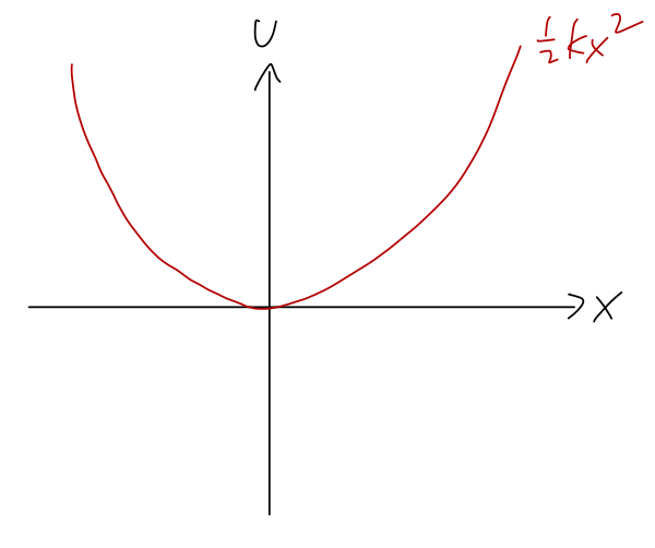
Again, the direction of the force is always “downhill”, opposite the direction of increasing U. We can also clearly see that there is an equilibrium point at x=0, where the potential is flat (dU/dx=0) and therefore the force vanishes. (Equilibrium just means that the system will stay there if we start it there at rest.)
The potential carries a lot of useful information about a physical system, even in cases where we can’t solve it completely! Once again, gravity will be a useful example and metaphor for understanding potentials in general. Imagine a roller coaster on a track. As a function of the distance x along the track, the height of the track y(x) will vary, usually in some complicated and interesting way. Since the gravitational potential is U(y) = +mgy, that means that drawing the track is the same thing as drawing the potential energy!
Suppose we have a segment of roller coaster track that looks like this:
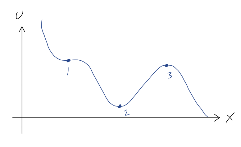
We can immediately see the points of equilibrium, marked 1, 2, and 3, where the force will vanish, and thus where the roller coaster cart would remain if it started at rest. We also get an immediate sense for the stability of these equilibria. A stable equilibrium point is one for which the system will remain near the equilibrium point if pushed slightly away; we can see that this is true at point 2, since if we give the cart a small push from this point, the force will always be directed back towards the lowest point.
An unstable equilibrium point is the opposite, a point where a small push will result in a large change in the system’s position. This is clearly the case at point 3; for a small push away from point 3, the force points away from point 3, and the coaster will accelerate away - back towards point 2, or off to the right, depending on which way we push it.
We can be more rigorous about these statements by considering a Taylor series expansion around each of these points. Let’s start with point 2, and I’ll use the shorthand notation U'(x) = dU/dx here. Since we already know that U'(x_2) = 0, the series expansion looks like U(x) \approx U(x_2) + \frac{1}{2} U''(x_2) (x-x_2)^2 + ... Now, we can’t actually compute the second derivative, but we do know from the plot that it must be positive. (Our series expansion is telling us that U(x) looks like a parabola if we get close enough to x_2, and from the plot the parabola has to be opening upwards.) So if we define U''(x_2) = +k with k>0, then U(x) \approx U(x_2) + \frac{1}{2} k(x-x_2)^2 + ... near point 2. Taking the derivative of this series gives us the force, F(x) = -\frac{dU}{dx} = -k(x-x_2). This looks exactly like a spring force; it points towards x_2, no matter what value of x we use. We can go a step further and solve for the motion. Let’s change coordinates so that u = x-x_2 is the distance to point 2. Then F(u) = -ku, and the equation of motion is m\ddot{u} = -ku. We haven’t considered general second-order ODEs yet, but we do know that this is a linear ODE, so it has a general solution containing 2 unknown constants, and we just need to find two different functions that go back to themselves with a minus sign after two derivatives. The basic trig functions both satisfy this property, so the solution is u(t) = A \cos (\sqrt{k/m} t) + B \sin (\sqrt{k/m} t). We don’t need any more detail than this: the point is that since \sin and \cos both oscillate between -1 and +1, our total solution is bounded - it will always stay within some range of point 2.
If we expand around point 3, we find an almost identical story, except that now we find U''(x_3) = -\kappa with \kappa > 0, which gives us the equation of motion m\ddot{u} = +\kappa u now with u = x-x_3. Without the minus sign, the solutions we find are exponentials instead of trig functions: u(t) = Ae^{-\sqrt{\kappa/m} t} + Be^{+\sqrt{\kappa/m} t}. The second exponential term gets arbitrarily large as t gets bigger, so our solution is indeed unstable - it will run away from point x_3. Of course, the motion isn’t exponential forever; we’re doing a series expansion around x_3, so as soon as we get far enough away that the terms we dropped from the series become important, we can’t use this simple solution for x(t) anymore.
Finally we come to point 1, which is sort of a tricky case; it is a saddle point of U(x), which means that the direction of the force depends on which way we push the cart. In physical terms, this is also an unstable equilibrium point. To see why, let’s Taylor expand one more time. We still know that U'(x_1) = 0, but we must also have U''(x_1) = 0. (You may remember from calculus that this is the condition for a saddle point. More physically, if U''(x_1) wasn’t zero, then close enough to x_1 our function would have to look parabolic, but that would mean it has to look like point 2 or point 3.) Thus, the series expansion here is U(x) \approx U(x_3) + \frac{1}{3!} U'''(x_3) (x-x_3)^3 + ... If we let U'''(x_3) = -q with q > 0 (convince yourself from the graph!), then the equation of motion is m\ddot{u} = \frac{1}{2} qu^2. We can’t solve this analytically - there is no solution using elementary functions. But we don’t need to, because it tells us what we need to know: the acceleration \ddot{u} is always positive, no matter the sign of u itself. So if we displace the cart from point 1 in either direction, it will be accelerated to the right - and since the acceleration increases as u increases, this solution is unstable and the cart moves away from point 1.
4.3.1 Total energy and turning points
Equilibrium points are local statements about a physical system, but we can also say interesting and useful things about the global behavior using the one-dimensional potential.
Let’s recap: since total energy E = T + U is conserved, if we know U(x) and the total energy, then we also know T(x). Instead of making a new plot, it’s often useful to just draw the value of E as a dotted line on the plot for U(x).
For example, let’s go back to our roller coaster and suppose the system begins at rest halfway between points 1 and 2. Then E = U(x_0), since at rest T=0. Let’s draw it on the graph:
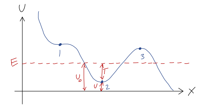
Since E = T + U and E is always the same, the difference between our dashed E line and the U(x) curve at any point is exactly the kinetic energy T! Now, since T = mv^2/2, it has the very important property that it can never be negative (note that U can be negative, and so can E, because the value U=0 is arbitrary.) But that means that we can never have U > E. So for the value of E shown, the cart can never reach point 1, point 3, or any part of the track above E!
This is a very simple but powerful observation: without knowing any of the details about how the cart moves with time, we know that its motion will never take it beyond the values of x where E = U(x) (the turning points.) The regions of the track where U > E are known as forbidden regions; we know the cart can never be found there. If all we know is E, then the cart could be anywhere else; in this example, it could be in the potential well near point 2, or it could be on the downward-sloping track to the right of point 3. If we also know where the cart starts, then we can identify it as being stuck in one of these two regions, and it can never get to the other one. (Of course, as you know from modern physics, this is only true classically; a quantum roller coaster would be able to tunnel from one region to the other.)
Here, you should complete Tutorial 4D on “One-dimensional potentials”. (Tutorials are not included with these lecture notes; if you’re in the class, you will find them on Canvas.)
We’ve previously talked about the motion of a simple pendulum, and found the equation of motion awhile ago to be \ddot{\phi} = -\frac{g}{L} \sin \phi
This is a non-linear differential equation, and there is no simple analytic solution to it at all. The usual procedure is to use the small-angle approximation, or numerical solution. But since this is a one-dimensional problem, we can instead write down the potential energy to make some useful observations!
Once again, here’s a sketch of the pendulum setup:
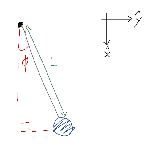
The only force acting is gravity, in the \hat{x} direction as the coordinates are drawn. Let’s set the gravitational potential to be zero at the lowest point of the pendulum, when \phi = 0. With the origin at the pendulum support, we thus have U(x,y) = mg(L-x) = mgL(1 - \cos \phi) using x = L \cos \phi. It’s always a good idea to check that the sign makes sense here, so let’s think about it: at \phi = 0, we have U = 0 as desired. At \phi = \pi/2, we have U = mgL; the gravitational potential should be larger when the bob is higher, so this also checks out.
Let’s sketch the potential as \phi changes from 0 to 2\pi:
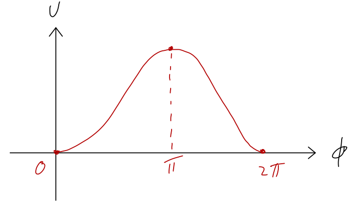
So we see two equilibrium points: in addition to the expected \phi = 0, there is also an unstable equilibrium at \phi = \pi. This might seem a little weird, but if you think about it for a moment it makes intuitive sense: at exactly \phi = \pi the pendulum is perfectly balanced straight above the support.
Although it’s easy to see graphically, let’s exercise our Taylor series abilities to check the stability or instability of the two equilibrium points. To find equilibrium points in general, we solve for where the gradient of U vanishes, or: \frac{dU}{d\phi} = 0 = mgL \sin \phi which has solutions at \phi = 0, \pi, 2\pi, ..., matching the points I already marked on the graph. Next, if we series expand the potential first at \phi = 0, we have U(\phi) \approx U(0) + \frac{1}{2} U''(0) \phi^2 + ... \\ = mgL(1 - \cos 0) + \frac{1}{2} (mgL \cos 0) \phi^2 + ... \\ = \frac{1}{2} mgL \phi^2 + ... which is indeed a stable equilibrium, since the coefficient of \phi^2 is positive. Note that I skipped the U' term in the expansion, since I already know it’s zero at this point. Let’s repeat the exercise at \phi = \pi, U(\phi) \approx U(\pi) + \frac{1}{2} U''(\pi) (\phi-\pi)^2 + ... \\ = mgL(1 - \cos \pi) + \frac{1}{2} (mgL \cos \pi) (\phi-\pi)^2 + ... \\ = 2mgL - \frac{1}{2} mgL (\phi-\pi)^2 + ... which is indeed unstable: the potential looks like a downwards parabola near the point, and if we compute the force F(\phi) = -\frac{dU}{d\phi} = mgL(\phi - \pi) it will always point in the same direction as \phi if we move slightly away from the equilibrium, and we will be pushed away.
Moving beyond equilibrium, we can also use conservation of energy and turning points to say useful things about the motion, without having to assume a small angle. Suppose the pendulum starts at \phi = 0, and we give it a push so that it starts moving with initial speed v_0. What does its motion look like? The total energy is just T at \phi = 0, so we have E = T + U \\ \frac{1}{2} mv_0^2 = T + mgL(1 - \cos \phi) The turning points \phi_T occur where T = 0, or \frac{1}{2} mv_0^2 = mgL (1 - \cos \phi_T) \\ 1 - \cos \phi_T = \frac{v_0^2}{2gL} \\ \Rightarrow \cos \phi_T = \left( 1 - \frac{v_0^2}{2gL} \right). So although we don’t know the detailed motion as a function of time, it’s easy to find the maximum possible angle the pendulum will reach based on the initial speed. Notice that this works for any angle, but only for v_0^2 < 4gL, at which point \phi_T = \pi. For even larger initial speeds, there is no solution: we just have E > U everywhere, and the pendulum will just spin in a circle forever, in the absence of other forces.
If we really want to know about the motion as a function of time, there’s one more nice trick we can do in one dimension. For any potential at all, the relation E = T + U in one dimension can be rewritten as: \frac{1}{2} m \dot{x}^2 = E - U(x). which we can solve for \dot{x}: \dot{x} = \pm \sqrt{\frac{2}{m}} \sqrt{E - U(x)} (we would need extra information to figure out the sign, since T is the same for +\dot{x} and -\dot{x}.) This is a first order and separable ODE - no matter how complicated U(x) is! So we can use it to write down a completely general solution: if x(0) = x_0, then t(x) = \pm \sqrt{\frac{m}{2}} \int_{x_0}^x \frac{dx'}{\sqrt{E-U(x')}} which we then have to invert to get x(t).
For the pendulum, this becomes t(\phi) = \pm \sqrt{\frac{m}{2}} \int_{\phi_0}^\phi \frac{d\phi'}{\sqrt{E - mgL(1 - \cos \phi')}} This is, unfortunately, one of those integrals that you can’t actually do: it is used to define a special function called an elliptic function, which is the solution to the pendulum at all angles. So we didn’t get something for nothing in this case. On the other hand, this can be a convenient way to do a numerical solution, since you don’t need an ODE solver like Mathematica - you just need to do an integral.
Here, you should complete Tutorial 4E on “One-dimensional potentials (part 2): Morse potential”. (Tutorials are not included with these lecture notes; if you’re in the class, you will find them on Canvas.)
Taylor explores a few other special topics in energy conservation, including the use of time-dependent potential energies (Taylor 4.5) and some more explorations of equilibrium and one-dimensional systems (4.7); I encourage you to read about these for your interest, but we won’t go into them in any detail. Instead, we’ll continue with his discussion of central forces, which will lead us into a detailed case study of the most important fundamental force in mechanics: gravity.
4.4 Central forces
A central force is one for which in some choice of coordinates, \vec{F}(\vec{r}) = f(\vec{r}) \hat{r}. The key point here is that the origin (i.e. the center of our coordinate system) is the source providing our central force, and the force at any point \vec{r} always points towards or away from this center. This should remind you a bit of drag forces, which we argued were always in the direction of \hat{v} (or opposite \hat{v}, more precisely.) In both cases, we have a specific direction for the force by identifying where it comes from (motion for air resistance, and the source object for central force.)
We’ll deal with gravity in great detail soon. Another good example that you already know of a central force is just the electric force: if I put a charge Q at the origin, then the force on a second charge q sitting at point \vec{r} is \vec{F}_e(\vec{r}) = \frac{kqQ}{r^2} \hat{r}. As Taylor observes, this (along with gravity, which has the same r dependence) is a slightly more specialized version of a central force, because f(\vec{r}) = f(r), i.e. the magnitude of the force only depends on the distance between the charges. This is an example of spherical symmetry, or rotational invariance: in spherical coordinates, we can rotate our test charge q around in \theta and \phi as much as we want, and as long as r is held fixed the force magnitude is the same (although the direction changes so it’s always pointing out from the origin.) As we’ll prove in a moment, this is related to the question of whether or not we have a conservative central force. A static electric force is definitely conservative!
4.4.1 Gradient and curl in spherical coordinates
To study central forces, it will be easiest to set things up in spherical coordinates, which means we need to see how the curl and gradient change from Cartesian. Let’s talk through the derivation for the gradient - although this is something you can always look up, it’s actually pretty easy, and the formula that you look up won’t seem so arbitrary. Remember that in our derivation of gradient, we found the following infinitesmal relationship: dU = \vec{\nabla} U \cdot d\vec{r}. To proceed, we need d\vec{r} in spherical coordinates. The derivation in full is included below, if you want to see it - it’s not that bad, but it requires a bit of algebra. The result is: d\vec{r} = dr\ \hat{r} + r d\theta\ \hat{\theta} + r \sin \theta\ d\phi\ \hat{\phi}.
We start with the observation that in spherical coordinates, \vec{r} = r\hat{r}. Taking the derivative with respect to some parameter s, \frac{d\vec{r}}{ds} = \frac{dr}{ds} \hat{r} + r \frac{d\hat{r}}{ds}. Next, we can relate the unit vector \hat{r} back to Cartesian coordinates: \hat{r} = \frac{1}{r} \left( x \hat{x} + y \hat{y} + z \hat{z} \right) \\ = \sin \theta \cos \phi \hat{x} + \sin \theta \sin \phi \hat{y} + \cos \theta \hat{z}. We can take a derivative with respect to s here, but it’s better to remember that we eventually want our answer in terms of spherical unit vectors. Remember that we define the unit vectors as pointing in the direction of change with respect to a certain coordinate, so we can find them by looking at the derivatives of \hat{r}: \frac{d\hat{r}}{d\theta} = \cos \theta \cos \phi \hat{x} + \cos \theta \sin \phi \hat{y} - \sin \theta \hat{z} \\ \frac{d\hat{r}}{d\phi} = - \sin \theta \sin \phi \hat{x} + \sin \theta \cos \phi \hat{y} and computing the lengths, \left| \frac{d\hat{r}}{d\theta} \right| = \cos^2 \theta (\cos^2 \phi + \sin^2 \phi) + \sin^2 \theta = 1 \\ \left| \frac{d\hat{r}}{d\phi} \right| = \sin^2 \theta (\sin^2 \phi + \cos^2 \phi) = \sin^2 \theta Now we use the chain rule: \frac{d\hat{r}}{ds} = \frac{d\hat{r}}{d\theta} \frac{d\theta}{ds} + \frac{d\hat{r}}{d\phi} \frac{d\phi}{ds} \\ = \left| \frac{d\hat{r}}{d\theta} \right| \hat{\theta} \frac{d\theta}{ds} + \left| \frac{d\hat{r}}{d\phi} \right| \hat{\phi} \frac{d\phi}{ds} on the last line using the definition of the unit vectors, \hat{\theta} = \frac{d\vec{r}/d\theta}{|d\vec{r}/d\theta|} = \frac{d\hat{r}/d\theta}{|d\hat{r}/d\theta|} where the second equality comes from the fact that the difference between \vec{r} and \hat{r} is a factor of the radius r, which doesn’t depend on the angle and so just cancels out. Combining our results above, we have \frac{d\hat{r}}{ds} = \frac{d\theta}{ds} \hat{\theta} + \sin \theta \frac{d\phi}{ds} \hat{\phi} or going all the way back to the start and cancelling out the ds infinitesmals, d\vec{r} = dr \hat{r} + r d\theta \hat{\theta} + r \sin \theta d\phi \hat{\phi}. This was a little bit of an algebra grind, but it’s been a little while since we’ve done these sorts of coordinate manipulations so I thought the practice would be good!
If you prefer a geometric derivation, Taylor does it that way without the algebra. In fact, it’s pretty easy to see that this form makes sense from a little sketch:
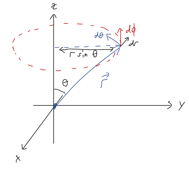
At fixed r, in the \theta direction, we’re always moving around a big circle of radius r, so the infinitesmal arc length that we travel is ds = r d\theta. In the \phi direction we’re also tracing out a circle, but the size of that circle depends on \theta, so ds = \rho d\phi = r \sin \theta d\phi.
Next, to work out how the function U changes with respect to coordinates, we just apply the chain rule to find dU = \frac{\partial U}{\partial r} dr + \frac{\partial U}{\partial \theta} d\theta + \frac{\partial U}{\partial \phi} d\phi. Notice there are no extra factors or coordinate changes to worry about - since U is just a scalar function, the chain rule applies in this same simple way no matter what! Now we rewrite the original equation: dU = \vec{\nabla} U \cdot d\vec{r} \\ \frac{\partial U}{\partial r} dr + \frac{\partial U}{\partial \theta} d\theta + \frac{\partial U}{\partial \phi} d\phi = (\vec {\nabla} U) \cdot \left( dr \hat{r} + r d\theta \hat{\theta} +r \sin \theta d\phi \hat{\phi} \right) and just matching the dr, d\theta, d\phi terms on both sides, we find \vec{\nabla} U = \frac{\partial U}{\partial r} \hat{r} + \frac{1}{r} \frac{\partial U}{\partial \theta} \hat{\theta} + \frac{1}{r \sin \theta} \frac{\partial U}{\partial \phi} \hat{\phi}.
Not bad at all! The bad news is that we can’t simply derive the curl or divergence from the gradient in spherical or cylindrical coordinates. This is basically for the same reason that Newton’s laws become more complicated in these coordinate systems: the unit vectors themselves become coordinate-dependent, so extra terms start to pop up related to derivatives acting on unit vectors.
The correct way to derive the curl in spherical coordinates would be to start with the Cartesian version and carefully substitute in our coordinate changes for the unit vectors and for (x,y,z) \rightarrow (r,\theta,\phi). This is straightforward but tedious, so I’ll skip to the result: the curl in spherical coordinates takes the form, in determinant notation, \vec{\nabla} \times \vec{A} = \frac{1}{r^2 \sin \theta} \left| \begin{array}{ccc} \hat{r} & r \hat{\theta} & r \sin \theta \hat{\phi} \\ \frac{\partial}{\partial r} & \frac{\partial}{\partial \theta} & \frac{\partial}{\partial \phi} \\ A_r & r A_\theta & r \sin \theta A_\phi \end{array} \right|
Let’s use this to compute the curl of central force vector \vec{F}(\vec{r}) = f(\vec{r}) \hat{r} in spherical coordinates: \vec{\nabla} \times \vec{F}(\vec{r}) = \frac{1}{r^2 \sin \theta} \left| \begin{array}{ccc} \hat{r} & r\hat{\theta} & r\sin \theta \hat{\phi} \\ \frac{\partial}{\partial r} & \frac{\partial}{\partial \theta} &\frac{\partial}{\partial \phi} \\ f(\vec{r}) & 0 & 0 \end{array} \right| \\ = \frac{1}{r \sin \theta} \frac{\partial f}{\partial \phi} \hat{\theta} - \frac{1}{r} \frac{\partial f}{\partial \theta} \hat{\phi}. So we can see right away that the condition for the curl to vanish - and therefore for \vec{F}(\vec{r}) to be conservative - is that both \partial f/\partial \phi and \partial f/\partial \theta should be zero, or in other words the magnitude should only depend on the radius, f(\vec{r}) = f(r). You can also prove this by using the gradient and matching on to the fact that \vec{F} has to point in the \hat{r} direction; convince yourself from the formula for \vec{\nabla} U we found, or read the argument in Taylor.
A central force \vec{F}(\vec{r}) = f(\vec{r}) \hat{r} is conservative if (and only if) it depends only on distance to the source: f(\vec{r}) = f(r).
4.4.2 Two-particle central forces
Conservative central forces are common in physics, particularly for fundamental forces: both electric force and gravitational force are central and conservative. One of the really nice features of such a force is that since the magnitude only depends on r, the distance to the source, many aspects of their physics can be treated as one-dimensional; we’ve already seen how that can be a really powerful simplification.
However, this setup so far forces a coordinate choice on us: we have to put our source at the origin. But what if we have two particles that are both sources, and are both moving - how can we describe their effects on each other through a central force? More generally, what if we have an extended source which is larger than a point - where do we put the origin?
We’ll start by generalizing to the two-particle case, which will be the hard part; taking the next step to extended sources will be easy. We start with two particles labelled 1 and 2, at positions \vec{r}_1 and \vec{r}_2 like this:
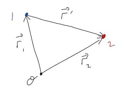
No external forces are present, but as shown, we assume that the particles are exerting a central force on one another. Defining the \hat{r}' vector pointing from 1 to 2 as shown, we have from the definition of a central force \vec{F}_{12} = f(\vec{r}') \hat{r}' \\ \vec{F}_{21} = -f(\vec{r}') \hat{r}' where we notice that Newton’s third law requires the magnitude to be the same function, so that these are equal and opposite. Now, \vec{r}' isn’t some unknown, it’s related to the positions of our two objects: \vec{r}' = \vec{r}_1 - \vec{r}_2 (easier to see in the form \vec{r}_1 + \vec{r}' = \vec{r}_2), and for the corresponding unit vector \hat{r}' = \frac{\vec{r}'}{|\vec{r}'|} = \frac{\vec{r}_1 - \vec{r}_2}{|\vec{r}_1 - \vec{r}_2|}. Since the central force only acts in the \vec{r}' direction, the point is that we can just solve for the relative motion of our two objects, and we’re back to having just one vector to worry about instead of two. So we don’t have to push one object to the origin for a central force to be a useful description of two objects - we just focus on their relative position.
You might object that just knowing the relative position isn’t enough information! We have two particles, which means we need 6 numbers to describe where they both are at any given moment, but \vec{r}' only has three components. In fact, we can get the other three components using the center of mass: because we’ve specified no external forces, we have for the CM position M \ddot{\vec{R}} = \vec{F}_{\textrm{ext}} = 0 which gives us the other three equations we need to fully keep track of everything.
What if we have not just a central force, but a conservative force? We know that f(\vec{r}') becomes just f(r') - that is, the force will only depend on the distance between our two particles and nothing else. As a result, we can write a single potential energy function U(r') that will describe the force f(\vec{r}')!
To get the individual forces from the potential, we take gradients with respect to each coordinate: \vec{F}_{12} = -\vec{\nabla}_1 U(r') \\ \vec{F}_{21} = -\vec{\nabla}_2 U(r') where the subscript gradient means “take derivatives with respect to the given coordinate”, for example in Cartesian coordinates \vec{\nabla}_1 = \frac{\partial}{\partial x_1} \hat{x}_1 + \frac{\partial}{\partial y_1} \hat{y}_1 + \frac{\partial}{\partial z_1} \hat{z}_1 ignoring the coordinates of \vec{r}_2. It’s easy to show from the definition of \vec{r}' that this definition gives us equal and opposite forces as required by the third law (try it yourself!)
Taylor has a very thorough discussion of how all of this generalizes beyond two particles, to the general N-particle case: the punchline is that we can always define a combined potential energy U for all our particles, and the force on any given particle is \vec{F}_\alpha = -\vec{\nabla}_\alpha U(\vec{r}_1, \vec{r}_2, ..., \vec{r}_N) and the total energy E = T_1 + T_2 + ... + T_N + U is always conserved (if the forces involved are conservative - which we’ve sort of assumed by writing a U in the first place, but there are some edge cases like time-dependent potential energies that Taylor talks about.)
I will just let you read the Taylor derivation and not go over it here; it’s an important fundamental result, but it doesn’t really show off any math that we haven’t seen before, and it’s not something we’ll need to work with practically. But the upshot is very important:
Given a conservative, central force, the combined force on a single point mass (at position \vec{r}) due to all other sources in the system can be described in terms of a single potential energy function U(\vec{r}).
This is a very useful observation, because it lets us deal with extended sources - realistic objects that emit a force, instead of only point sources. With this result in hand, let’s move on to consider a single conservative, central force in detail: gravity!
4.5 Gravity
Our starting point is Newton’s general law of gravitation. If we have a source mass M at the origin, and a test mass m at \vec{r}, the force of gravity acting on the test mass is \vec{F}_g = -\frac{GMm}{r^2} \hat{r}. The “gravitational charge” of an object is just its mass. Since mass is always positive, the force of gravity is always attractive - it pulls the two objects together, or in this case, pulls the mass m towards M at the origin. The constant G is known as the gravitational constant, Newton’s constant or just “big G”; its best value, according to NIST CODATA, is G = 6.67430(15) \times 10^{-11}\ {\textrm{m}}^3 / {\textrm{kg}} / {\textrm{s}}^2. The corresponding potential energy function is U(r) = -\frac{GMm}{r} We can add an arbitrary constant to it; the choice above with no constant corresponds to choosing our zero point at infinity, i.e. \lim_{r \rightarrow \infty} U(r) = 0.
Take special note that both \vec{F}_g and U(r) are negative, despite the relationship \vec{F} = -\nabla U! Mathematically, this happens because the derivative of 1/r pops out a extra minus sign, which cancels the other minus sign in the definition of force. You can also remember the sign on physical grounds: it takes work to push two massive objects apart against gravity, so U should increase as r increases, which it does with the minus sign.
The gravitational force closely resembles the electric force, and in a similar way to the electric example, we can define a gravitational field \vec{g} by dividing out the “charge” (the mass in this case), such that \vec{F}_g = m\vec{g}. From above, the gravitational field generated by a point mass M is then \vec{g} = -\frac{GM}{r^2} \hat{r}.
There isn’t a whole lot of interesting physics we can do with just two masses, as it turns out. (Well, we could derive Kepler’s laws for the motion of planets in the solar system, but that turns out to be much nicer with some extra math tools that you’ll get next semester.) So what happens if we have multiple sources? Since multiple forces acting on a simple object just add together, we can also add together the gravitational fields from multiple sources to get a single, combined field: \vec{g} = \vec{g}_1 + \vec{g}_2 + ... = -\frac{GM_1}{r_1^2} \hat{r}_1 -\frac{GM_2}{r_2^2} \hat{r}_2 + ...
This is the starting point we need to talk about extended sources, which will let us do some realistic applications of gravity, such as the Earth’s gravitational field.
4.5.1 Extended sources of gravity
To deal with realistic objects, we’d like to be able to calculate the gravitational field due to a continuous object with some density. Recalling our previous example of finding the center of mass, we can think of this as just adding up all of the contributions from infinitesmal bits of mass dm inside of an object. For the center of mass, recall we had M = \sum_\alpha m_\alpha,\ \ \vec{R} = \frac{1}{M} \sum_\alpha m_\alpha \vec{r}_\alpha which became for continuous objects M = \int dm = \int \rho(\vec{r}) dV,\\ \vec{R} = \frac{1}{M} \int \vec{r} dm = \frac{1}{M} \int \vec{r} \rho(\vec{r}) dV.
Similarly, for an extended massive source, we can add up all of the contributions to the gravitational field from individual pieces. However, this is going to be a little more complicated, so we should start with a diagram:
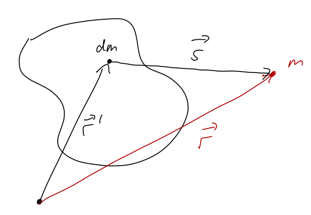
As pictured, we have to keep track of the location \vec{r}' of our source mass, but also the position \vec{r} where we want to know the field. As a sum over individual masses m_\alpha, we have
\vec{g} = \sum_\alpha -\frac{Gm_\alpha}{|\vec{s}_\alpha|^2} \hat{s}_\alpha where \vec{s} = \vec{r} - \vec{r}'_\alpha is the vector pointing from the source mass \alpha to the position \vec{r}. (Some books will refer to this using a funny-looking script r; I think this is confusing, and I also don’t know how to typeset the weird r, so I’ll use s.)
We find the continuous version by replacing m with the density \rho: \vec{g}(\vec{r}) = -G \int \frac{dm}{|\vec{s}|^2} \hat{s} \\ = -G \int \frac{dV' \rho(\vec{r}')}{|\vec{r} - \vec{r}'|^3} (\vec{r} - \vec{r}') where I’ve written out \hat{s} in terms of the other vectors, which gives us an extra factor of 1/|\vec{s}|. As the prime on dV' indicates, we’re integrating over all possible positions \vec{r'} of the source mass dm. We can do a u-substitution to think of the integral as being over the relative position vector \vec{s}, but that hides the dependence on \vec{r'} which can be confusing.
This looks pretty horrible compared to the center of mass integral! Much of the complication comes from the fact that we have a second vector \vec{r} in addition to the one that we’re trying to integrate over. We’ll do a couple of examples, but I’ll emphasize from the start that it is very important to make sketches and think carefully about these vectors when trying to calculate \vec{g}!
Symmetry will also be very useful, as with the center of mass. In particular, suppose we are at the origin and there are two equal pieces of mass at +\vec{s} and -\vec{s}, exactly on opposite sides:
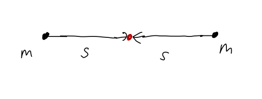
Then the total gravitational field is, taking the horizontal direction to be the x-axis, \vec{g} = -\frac{Gm}{s^2} \hat{x} - \frac{Gm}{s^2} (-\hat{x}) = 0. In other words, just as we saw for the CM position, the contributions of two equal masses at opposite positions to the \vec{g} field cancel exactly. This reflection-symmetry observation will extend to a whole object: if we have two solid hemispheres with the same mass and shape, then at the point exactly in between their centers, \vec{g} = 0 without having to calculate anything.
This can also work component by component. If we have our two equal masses at (+x',0,0) and (-x',0,0), and we’re interested in the gravitational field along the y axis:
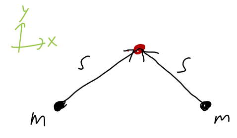
The distance s to both sources is the same again, but now the directions are slightly different. Worrying about the \hat{s} vector (which we’ll define with respect to the left source to be consistent with signs), we have:
g_x = -\frac{GM}{s^2} (\hat{s}_x - \hat{s}_x) = 0, \\ g_y = -\frac{GM}{s^2} (\hat{s}_y + \hat{s}_y) \neq 0.
In words: the magnitude of the field is the same from both sources, but the y-components add since they both point in the same direction (downwards), so g_y is not zero.
Here, you should complete Tutorial 4F on “Gravitational fields”. (Tutorials are not included with these lecture notes; if you’re in the class, you will find them on Canvas.)
Let’s try to apply our setup to a real example of finding \vec{g} for an extended object (not just point masses.) Suppose we have a solid but very thin disk of constant area mass density \sigma and radius R.
To deal with a thin disk, our integral over dV will become just a two-dimensional area integral dA, since the z-direction is infinitesmally thin. (If you’re not happy with this hand-waving approximation, you can calculate the three-dimensional version of this for a height h, and then take the limit h \rightarrow 0. You should get the same results we’re about to find.)
Now, as with the center of mass, we can view the equation for \vec{g} as just three separate integrals to do for each of the components g_x, g_y, g_z. In general, we need to calculate all three of them, but symmetry can save us by telling us certain components are automatically zero. However, things are complicated by the fact that we have to choose the point \vec{r} to calculate the field at. For a completely arbitrary point in space, symmetry won’t help us for the disk!
But let’s say we want to calculate the field directly above the center of the disk, along the z-axis:
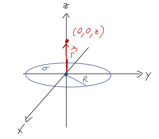
Then we have \vec{g}_x = \vec{g}_y = 0 thanks to reflection symmetry (remember, it’s the reflection of the relative \vec{s} vector that matters, which is why we had to specify \vec{r} = z\hat{z} first!) Let’s convince ourselves by actually setting up one of the integrals: g_x = -G \int \frac{dA' \sigma}{|\vec{r} - \vec{r}'|^3} (\vec{r} - \vec{r}')_x \\ = G \sigma \int \frac{dA' x'}{(x'^2 + y'^2 + z^2)^{3/2}} using \vec{r} - \vec{r}' = -x' \hat{x} - y' \hat{y} + z \hat{z}, from the diagram. Now, this is already good enough to see the cancellation: because the integrand has a single x' upstairs, for every point on the disk at (+x', +y') there will be an equal and opposite contribution from (-x',y'), so the whole thing will be zero. To see it even more explicitly, we should really change to cylindrical coordinates (\rho', \phi') inside the integral: g_x = G \sigma \int_0^{2\pi} d\phi' \int_0^R d\rho' \frac{\rho'^2 \cos \phi'}{(\rho'^2 + z^2)^{3/2}} The \phi' integral is the one that matters, and it’s easy to do: we have \int_0^{2\pi} d\phi' \cos \phi' = \left. \sin \phi'\right|_0^{2\pi} = 0.
Since the choice of x-direction vs. y-direction on a disk is totally arbitrary, clearly the same setup will give us g_y = 0 as well.
Now let’s move on to the non-zero part of the field, g_z. Since we’ve already gone through the details of the setup for x, it should be easy to see that g_z = -G \sigma \int_0^{2\pi} d\phi' \int_0^R d\rho' \frac{\rho' z}{(\rho'^2 + z^2)^{3/2}} \\ = -2\pi G \sigma z \int_0^R \frac{d\rho' \rho'}{(\rho'^2 + z^2)^{3/2}}. This is actually a very friendly integral for u-substitution! Let’s pick u = \rho'^2 + z^2, which gives du = 2\rho' d\rho'. Then g_z = -2\pi G \sigma z \int_{z^2}^{R^2 + z^2} \frac{du/2}{u^{3/2}} \\ = -\pi G \sigma z \left( \left. -\frac{2}{u^{1/2}} \right|_{z^2}^{R^2+z^2} \right) \\ = 2\pi G \sigma z \left( \frac{1}{\sqrt{R^2 + z^2}} - \frac{1}{|z|} \right). \\ We could replace the density \sigma with the total mass M; since it’s a two-dimensional density, we have M = \sigma \pi R^2. But there’s no normalizing 1/M like there is for the center of mass, so for this calculation it’s fine to just leave it in terms of \sigma in general.
The other limit to consider is z \rightarrow \infty. This means that z \gg R, which we can use to series expand the first term in the field: \frac{1}{\sqrt{R^2 + z^2}} = \frac{1}{|z|} \frac{1}{\sqrt{1 + (R/z)^2}} Let’s use the binomial formula to expand, (1+z)^n = 1 + nz + \frac{n(n-1)}{2} z^2 + ... which leads to, just keeping the first two terms, \frac{1}{\sqrt{R^2 + z^2}} \approx \frac{1}{|z|} \left(1 - \frac{R^2}{2z^2} + ... \right) The 1/|z| terms cancel off, and we’re left with g_z \rightarrow 2\pi G \sigma \frac{z}{|z|} \left( -\frac{R^2}{2z^2} + ... \right) Now it’s useful to substitute in M = \pi R^2 \sigma, which will absorb the R^2 factor and leave us with g_z \rightarrow -\frac{GM}{z^2} \frac{z}{|z|} or \vec{g} = -GM/z^2 \hat{r}, along the z-axis. So in this limit, the leading dependence on R vanishes and we just recover the single point-particle form of the gravitational field! This makes a lot of sense: if we’re really, really far away from the disk, then the fact that it’s an extended object doesn’t really matter - in fact, from far enough away we probably wouldn’t be able to tell that it has any radius, we would just see a point.
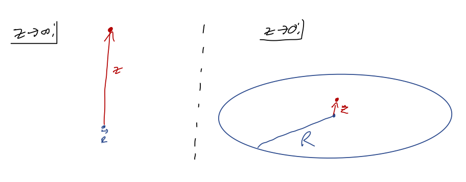
4.5.2 Gravitational potential
So far, we haven’t really used the fact that gravity is a conservative force. In fact, being able to write a potential energy function U(\vec{r}) can actually save us a lot of work when dealing with extended objects! Recall that the potential energy for a single test mass m in the gravity field of a source mass M is U(r) = -\frac{GMm}{r}. When we have multiple sources, as we discussed above for any conservative central force, we simply add up the potentials!
One more definition before we continue: like the force, the potential energy depends on the test mass m, but in a very trivial way. It’s often useful to factor out the m so we can calculate a function that only depends on the sources, which we can then apply to any test mass (or collection of test masses.) So just like we defined \vec{F}_g = m\vec{g}, we now define the gravitational potential for a point source to be \Phi(r) = -\frac{GM}{r} so that U(r) = m\Phi(r). We can immediately see that \vec{g} = -\vec{\nabla} \Phi, so this gives us another way to find the gravitational field.
Potential is an unfortunate name for the quantity \Phi; it is not a potential energy, since it has the wrong units! Taking the combination U = m\Phi gives us an actual potential energy. This is completely analogous to the electric potential V(r), which is also not a potential energy - but the combination qV is.
Now if we have an extended object, as we saw before:
then the potential at position \vec{r} due to the infinitesmal source dm is d\Phi(\vec{r}) = -\frac{G dm}{s} = -\frac{G dm}{|\vec{r} - \vec{r}'|}, and thus the total potential is \Phi(\vec{r}) = -G \int \frac{dV' \rho(\vec{r}')}{|\vec{r} - \vec{r}'|}. This is much nicer to evaluate than the integrals we had to do for \vec{g}! Now we have no vector components to worry about - just a single scalar quantity. We can then take the gradient of our result (with respect to \vec{r}) to find the gravitational field \vec{g}.
Here, you should complete Tutorial 4G on “Gravitational potential”. (Tutorials are not included with these lecture notes; if you’re in the class, you will find them on Canvas.)
Now let’s do an example to see how this approach works in more detail.
Let’s find the \vec{g} field due to a spherical shell of mass M (and constant mass density \sigma), using the gravitational potential \Phi. Once again, we’ll consider a target point on the z-axis, so \vec{r} = z\hat{z}.
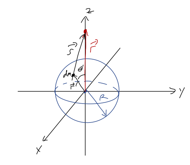
We start by setting up the integral, using the sketch as a guide: \Phi(\vec{r}) = -G \int \frac{dA' \sigma}{|\vec{r} - \vec{r}'|}. Let’s work in spherical coordinates since we have a sphere. The vector \vec{r}' has length R, but is at arbitrary spherical angles \theta, \phi. In order to proceed, we’ll need to find the length of the vector \vec{r} - \vec{r}'. The geometry is a bit tricky, although if you make a sketch and remember the law of cosines, it’s straightforward to find.
I personally can never remember the law of cosines, so I prefer to just write out the two vectors and take the difference! Using spherical coordinates but Cartesian basis vectors, we have:
\vec{r}' = R \sin \theta' \cos \phi' \hat{x} + R \sin \theta' \sin \phi' \hat{y} + R \cos \theta' \hat{z} and much more simply, \vec{r} = z \hat{z}. So, taking the difference and then the squared length: |\vec{r} - \vec{r}'|^2 = (r' \sin \theta' \cos \phi')^2 + (r' \sin \theta' \sin \phi')^2 + (z - r' \cos \theta')^2 \\ = r'^2 + z^2 - 2zr'\cos \theta'.
You might wonder, why are we mixing spherical and Cartesian coordinates here, instead of just working with spherical basis vectors as well? The reason is that spherical basis is great for any single vector, but with two vectors to deal with here it’s not so useful!
In spherical coordinates, the reference point is at \vec{r} = z \hat{\rho}, and the object point is at \vec{r}' = R \hat{\rho}'. But since these are two different vectors, they have two different spherical unit vectors! We could try to figure out how \hat{\rho} and \hat{\rho}' are related, but we need a common set of basis vectors to do it - probably just the Cartesian basis we’re using anyway for this problem.
Now we can set up our integral for \Phi(z). Since we’re working with a shell, this will be an area integral over the two spherical angles:
\Phi(z) = -G \sigma \int_0^{2\pi} d\phi' \int_0^\pi d\theta' \frac{R^2 \sin \theta'}{\sqrt{R^2 + z^2 - 2zR \cos \theta'}}.
The integral over \phi' is trivial, and just pops out a factor of 2\pi, so the only work we have left is the \theta' integral. This integral is actually a little tricky, simply because you have a good chance of getting stuck if you’re used to just plugging things in and letting Mathematica deal with them!
The good news is that there is a pretty obvious u-substitution to do. Since almost everything in the square root is constant, we can write u = R^2 + z^2 - 2zR \cos \theta' \Rightarrow du = 2zR \sin \theta' d\theta' The new limits of integration will be \theta'=0 \Rightarrow u=(z-R)^2, \\ \theta' = \pi \Rightarrow u = (z+R)^2.
With the \sin \theta' already upstairs, this simplifies really nicely: \Phi(z) = -2\pi \sigma G \int_{(z-R)^2}^{(z+R)^2} \frac{R^2 du}{2zR} \frac{1}{\sqrt{u}} \\ = -\pi \sigma G \frac{R}{z} \left(2 \left.\sqrt{u}\right|_{(z-R)^2}^{(z+R)^2}\right) \\ = -2\pi \sigma G \frac{R}{z} (z+R - (z - R)) \\ = -4\pi \sigma G \frac{R^2}{z}.
Some of these numerical factors should look familiar: the combination 4\pi R^2 is just the surface area A of the sphere, and since A \sigma = M, we have finally just \Phi(z) = -\frac{GM}{z}.
An important observation to make is that there is nothing special about the z direction for a sphere. If I chose a point in any arbitrary direction above the surface of the sphere to find the potential at, I could have just called that direction z and I would get the same answer.
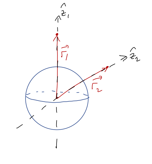
Thanks to this rotational symmetry, the z-axis answer is the answer everywhere: for any point a distance r>R from the center of the sphere, we have \Phi(r) = -\frac{GM}{r}. This is the same potential as if all of the mass were concentrated at the center of the sphere - even if we’re really close to the surface!
What about points inside the shell, instead (so z < R)? Most of the setup will be exactly the same; in fact, we need to be careful to even spot the difference! Our work will be exactly the same up to the following equation: \Phi(z) = -\pi \sigma G \frac{R}{z} \left( \left. 2 \sqrt{u} \right|_{(z-R)^2}^{(z+R)^2} \right). When we’re taking the square root, we have to make sure the result is positive. Before, we took \sqrt{u} \rightarrow z-R for the bottom limit of integration; this is positive as long as z > R. But now, we should take R-z instead, which leads to: \Phi(z) = -2\pi \sigma G \frac{R}{z} \left( R + z - (R-z) \right) \\ = -4\pi \sigma G R or in terms of total mass, \Phi(z) = -\frac{GM}{R}.
This is a constant, for any value of z (and thus due to spherical symmetry, for any point inside the sphere). Constant potential means the force due to gravity will be exactly zero!
The surprisingly simple results we found for the sphere and spherical shell above are actually consequences of some powerful math at work, which we’ll explore next.
4.5.3 Gauss’s law and gravity
We’ve emphasized that the potential tends to be easier to work with than trying to calculate \vec{g} directly. However, one good reason to use \vec{g} in certain cases is to invoke some very powerful results from vector calculus. We already mentioned Stokes’ theorem briefly in our discussion of curl and conservative forces. Now I’ll borrow another result, again without proof, known as Gauss’s law: \oint_{\partial V} \vec{g} \cdot d\vec{A} = -4\pi G \int_V \rho(\vec{r}) dV = -4\pi G M_{\textrm{enc}}. Let’s unpack the dense notation here, a lot of which looks very similar to Stokes’s theorem. Here V denotes some volume in three-dimensional space, and \partial V is the boundary of this volume, which must be a closed surface (in the same way that the boundary \partial A of a surface is a closed loop); the ring on the integral reminds us of this. We know what everything else is, except for M_{\textrm{enc}}: this is the “enclosed mass”, i.e. the total of all the mass contained in the region V.
Where does this result come from? To understand that, we need to introduce our last vector derivative, the divergence, which we get as the dot product of the gradient with another vector. In Cartesian coordinates, we would have \vec{\nabla} \cdot \vec{g} = \frac{\partial g_x}{\partial x} + \frac{\partial g_y}{\partial y} + \frac{\partial g_z}{\partial z} and the equivalents in cylindrical or spherical are more complicated - refer to the back of Taylor. Gauss’s law is actually a special case of a more general vector calculus result known as the divergence theorem, stated without proof: for any vector field \vec{b}(\vec{r}), the divergence theorem states that \oint_{\partial V} \vec{b}(\vec{r}) \cdot d\vec{A} = \int_V (\vec{\nabla} \cdot \vec{b}(\vec{r})) dV This matches on to Gauss’s law if we make the identification \vec{\nabla} \cdot \vec{g} = -4\pi G \rho(\vec{r}). This equation is sometimes also called Gauss’s law, because one version implies the other one thanks to the divergence theorem. This last equation is also interesting, because we can view it as a differential equation that can be solved for \vec{g} given \rho(\vec{r}) - yet another way to obtain the gravitational vector field!
Actually, there’s one more simplification we can make here. Remember that the gravitational field is related to the potential as \vec{g} = -\vec{\nabla} \Phi. If we plug this in, we find the equation \nabla^2 \Phi(\vec{r}) = 4\pi G \rho(\vec{r}), where \nabla^2 is another new operator called the Laplacian, which is basically the dot product of the gradient \vec{\nabla} with itself. In Cartesian coordinates, \nabla^2 \Phi = \frac{\partial^2 \Phi}{\partial x^2} + \frac{\partial^2 \Phi}{\partial y^2} + \frac{\partial^2 \Phi}{\partial z^2}. This differential equation relating \Phi directly to \rho is known as Poisson’s equation. For some applications, it’s the most convenient way to solve for the gravitational field, since we don’t have to worry about vectors at all: we get the scalar potential from the scalar density. In particular, Poisson’s equation is often a useful way to solve numerically for the potential due to a complicated source density.
We won’t use the differential versions of these equations in practice this semester, but they are very useful for more than just numerical solutions: you’ll probably see a lot of them when you take electricity and magnetism. But I wanted to explain in a bit more detail where Gauss’s law comes from.
Having covered the math, I should say a little bit more about the physical interpretation of Gauss’s law. The quantity on the left-hand side, \oint_{\partial V} \vec{g} \cdot d\vec{A}, is known as the gravitational flux through the surface \partial V. There are some hand-waving arguments people sometimes like to make about “counting field lines” to think about flux, but obviously this is a little inaccurate since the strength |\vec{g}| of the field matters and not just the geometry. Still, a physical way to state Gauss’s law is: “for a surface with no enclosed mass, the net gravitational flux through the surface is zero.”
How do we use Gauss’s law as a calculational tool? Dealing with the right-hand side is pretty easy; we know how to do integrals over density to find the mass already. But for the left-hand side, it’s not so obvious. The key will be to find a clever choice of our “Gaussian surface” \partial V, so that the product \vec{g} \cdot d\vec{A} will be constant. If this product is constant over the surface (ideally, if \vec{g} is parallel to d\vec{A}), then we can just pull out the magnitude of \vec{g} and the integral just becomes the surface area. Let’s see how it works with a simple example.
Let’s revisit our calculations for the case of a thin spherical shell of radius R and total mass M. We’ll begin by working outside the sphere, so r > R. We take a Gaussian spherical surface at r to match our spherical source:
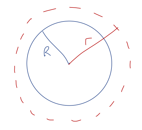
The spherical surface we’ve chosen here is known as a Gaussian surface - it defines the vector d\vec{A} and is crucial in applying Gauss’s law. We always want to choose the Gaussian surface to match the symmetries of our problem. Here, symmetry tells us immediately that \vec{g}(\vec{r}) = g(r) \hat{r} in the case of a spherical source. Since d\vec{A} is also in the \hat{r} direction for a spherical surface, we have \vec{g} \cdot d\vec{A} = g(r) dA, and then we can pull g(r) out of the integral. Thus, \oint_{\partial V} \vec{g} \cdot d\vec{A} = -4\pi G \int_V \rho(\vec{r}) dV becomes g(r) (4\pi r^2) = -4\pi G M \Rightarrow g(r) = -\frac{GM}{r^2}. This was way easier to find using Gauss’s law than the direct calculation we did! What about inside the spherical shell? For r < R, we again take a spherical surface:
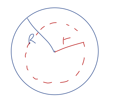
The entire calculation is the same as outside the sphere, except that now M_{\textrm{enc}} is always zero - correspondingly, we simply have g(r) = 0 for r < R. This again matches the result we found the hard way before - constant potential, which gives zero \vec{g} field when we take the gradient.
Here, you should complete Tutorial 4H on “Gauss’s law and dark matter”. (Tutorials are not included with these lecture notes; if you’re in the class, you will find them on Canvas.)
There aren’t a huge number of applications of Gauss’s law, in fact; the only three Gaussian surfaces that are commonly used are the sphere, the cylinder, and the box, matching problems with the corresponding symmetries (a sphere, a cylinder, or an infinite plane.) For most other cases (like this question), there simply isn’t quite enough symmetry to actually use Gauss’s law in practice. We will see one more very important application soon, when we talk about dark matter. In the rare cases where it does apply, it makes calculating \vec{g} really easy!
Before we move on, there is one really useful thing we can do with Gauss’s law even when dealing with an arbitrary object shape.
Here I’ll use Gauss’s law to prove a very general result that was hinted at by our solutions above: for any massive object of size R, the gravitational field at distances r \gg R will be exactly the field of a point mass and nothing more. Let’s draw a spherical surface of size r \gg R around our arbitrary object of mass M:
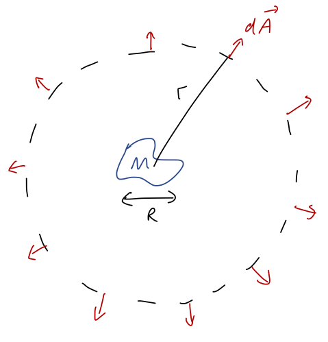
Since we don’t know what \vec{g}(\vec{r}) is yet, our objective is to choose the right simplifications so we can pull \vec{g} out of the integral on the left-hand side.
Since r is much larger than R, the volume integral on the right-hand side of Gauss’s law always includes the entire object, and we just get the total mass M. So in other words, for any choice of r > R, we have \oint_{\partial V} \vec{g}(\vec{r}) \cdot d\vec{A} = -4\pi G M. With our choice of a spherical surface as \partial V, the vector d\vec{A} is always in the \hat{r} direction. Explicitly in spherical coordinates, \int_0^{2\pi} d\phi \int_0^\pi d\theta (r^2 \sin \theta) \vec{g}(\vec{r}) \cdot \hat{r} = -4\pi G M Now let’s think about the field \vec{g}(\vec{r}). If our object were perfectly symmetric, like a sphere, then any components not in the radial direction would cancel off as we’ve seen, and we would have \vec{g}(\vec{r}) = g(r) \hat{r}. On the other hand, what if it wasn’t perfectly symmetric? That would mean we have an imperfect cancellation between the field contributions from two bits of mass that are no more than R apart from each other. But the contribution from two such pieces has to be something like |\Delta g(\vec{r})| \sim \frac{1}{|\vec{r}'_1 - \vec{r}|^2} - \frac{1}{|\vec{r}'_2 - \vec{r}|^2} \\ = \frac{1}{r^2} \left(1 + \frac{2|\vec{r}'_1|}{r} + ... \right) - \frac{1}{r^2} \left(1 + \frac{2|\vec{r}'_2|}{r} + ... \right) The 1/r^2 parts cancel off nicely, so the leading term is something like (|\vec{r}'_1| - |\vec{r}'_2|) / r^3. But this can’t be any larger than R/r^3, which is R/r smaller than the leading 1/r^2 term. In other words, we know that \vec{g}(\vec{r}) = g(r) \hat{r} + \mathcal{O} \left(\frac{R}{r} \right) even if our object isn’t spherically symmetric. If we only keep the leading term, then the integral simplifies drastically: -4\pi G M = \int_0^{2\pi} d\phi \int_0^\pi d\theta \sin \theta r^2 g(r) = 4\pi r^2 g(r) and since there’s no r-integral, we just have g(r) = -\frac{GM}{r^2} up to corrections of order R/r, as I assumed.
This is a nice confirmation of the arguments I made above, that everything looks like a point mass if you’re far enough away! It’s also a simple example of how we use Gauss’s law in practice: it’s most useful if some symmetry principle lets us identify the direction of g(r) so that we can actually do the integral on the left-hand side. If we try to keep even the leading R/r correction, we’ll have to find another way to get the answer, because it will have some dependence on the angle \theta in addition to the distance r.
You should recognize a lot of similarities between how we’re dealing with the gravitational force and how you’ve seen the electric force treated before. Here’s a quick list of equivalences between gravity and electric force:
Gravity vs. electric:
- Force: \vec{F}_g = -\frac{GMm}{r^2} \hat{r} vs. \vec{F}_e = +\frac{kQq}{r^2} \hat{r}
- Field: \vec{g} = \frac{\vec{F}_g}{m} = -\frac{GM}{r^2} \hat{r} vs. \vec{E} = \frac{F_e}{q} = \frac{kQ}{r^2} \hat{r}
- Potential energy: U(r) = -\frac{GMm}{r} vs. U(r) = +\frac{kQq}{r}
- Potential: \Phi = \frac{U}{m} = -\frac{GM}{r} vs. V = \frac{U}{q} = +\frac{kQ}{r}
and of course Gauss’s law: for gravity we have \oint_{\partial V} \vec{g} \cdot d\vec{A}' = -4\pi G \int_V \rho(\vec{r}') dV' = -4\pi G M_{\textrm{enc}}. while the electric version reads \oint_{\partial V} \vec{E} \cdot d\vec{A}' = +4\pi k Q_{\textrm{enc}}.
Notice how everything is almost completely identical! The main differences are a different constant (G vs. k), a different “charge” (m and M vs. q and Q), and the minus sign - reflecting the fact that like charges repel in electromagnetism, but they attract for gravity.
A lot of the tools and techniques we’re talking about now will transfer more or less directly to electromagnetism; for example, calculating the electric potential V(\vec{r}) from an extended charged object.
4.6 Selected modern topics in gravity
One of the more exciting things about teaching gravitation is that we now have the tools to make contact with some really important and cutting-edge ideas in physics! I’ll give you a taste of two such topics: effective theories, and dark matter.
4.6.1 Effective theory and gravity at the Earth’s surface
As we’ve just seen, to the extent that the Earth is a sphere, we know that its gravitational field on the surface and above is \vec{g}(r) = -\frac{GM}{r^2} \hat{r}.
However, this is not the form you use in the lab! For experiments on the Earth’s surface, we replace this with the constant acceleration g. In fact, we can derive this by expanding our more general result in the limit that we’re pretty close to the Earth’s surface.
Let R_E be the radius of the Earth, M_E its mass, and suppose that we conduct an experiment at a distance z above that radius. Then we have \vec{g}(z) = -\frac{GM_E}{(R_E+z)^2} \hat{z} = -g(z) \hat{z} where I’ve replaced \hat{r} with \hat{z}, because if we’re on the surface of a sphere, “up” is the same as the outwards radial direction. Now, if we assume that we’re relatively close to the surface so z \ll R_E, then a series expansion makes sense: g(z) = \frac{GM_E}{R_E^2 (1 + (z/R_E))^2 } = \frac{GM_E}{R_E^2} \left[ 1 - \frac{2z}{R_E} + \frac{3z^2}{R_E^2} + ... \right] We see that indeed, so long as z is very small compared to R_E, then g(z) \approx g, a constant acceleration. We can also see now where g comes from in terms of other constants; if we measure g \approx 9.8 {\textrm{m}}/{\textrm{s}}^2, and we also know G = 6.67 \times 10^{-11} {\textrm{m}}^3 / {\textrm{kg}} / {\textrm{s}}^2 and R_E \approx 6400 km = 6.4 \times 10^6 m, then we can find the mass of the Earth: M_E = \frac{gR_E^2}{G} \approx 6 \times 10^{24}\ {\textrm{kg}}. This is, essentially, the only way we have to measure M_E; the composition of the Earth is complicated and not well-understood beyond the upper layers that we can look at directly, so it’s hard to estimate using density times volume.
Our series expansion buys us a lot more than just estimating g! In particular, we have a specific prediction that if we change z by enough, we’ll be sensitive to a correction term linear in z g(z) \approx g \left(1 - \frac{2z}{R_E} + ... \right) Boulder is about 1.6km above sea level, so in this formula, we would predict that g is smaller by about 0.05% due to our increased height. This is a very small difference, but not so small that it can’t be measured! (Although there are other effects of similar size, including centrifugal force due to the fact that the Earth is spinning.)
Now we come to the big idea here, which is the idea of effective theory. This is something which is rarely taught in undergraduate physics, but I believe it’s one of the most important ideas in physics - and it’s lurking in a lot of what you are taught, even if we don’t acknowledge it by name.
My definition of an effective theory is that it is a physical theory which is agnostic about the true underlying physical model, on the basis of identifying a scale separation. If we are interested in some system of size r, then any physics relevant at much longer scales L \gg r is “separated”. So is any physics relevant at much shorter scales, \ell \ll r.
Going back to our example for g(z), we could also ask about the influence of the Sun’s gravity on an object on the Earth’s surface; this would depend on the Earth-Sun distance, R_{ES} = 1.48 \times 10^{11} m. Or maybe we’re worried about the quantum theory of gravity, and want to know the effect of corrections that occur at very short distances (our best modern estimate of the length scale at which this would matter is the Planck length, \ell_P = 1.6 \times 10^{-35} m.) Scale separation tells us that we can series expand such contributions in ratio to the scale z at which we’re experimenting: g(z) \approx g \left( 1 - \frac{2z}{R_E} + ... \right) + C_1 \frac{z}{R_{ES}} + C_2 \frac{\ell_P}{z} + ... and although we can keep these terms in our expansion, as long as the numerical coefficients C_1, C_2 aren’t incredibly, surprisingly large, the ratios z/R_{ES} and \ell_P/z are so incredibly small that we can always ignore such effects. So we can see the power of scale separation: large enough separation allows us to completely neglect other scales, because even their leading contribution in a series expansion would be tiny!
This validates the effective theory framework of ignoring any physical effects that are sufficiently well-separated, although it’s very important to note that this depends on z, the experimental scale. An effective theory doesn’t claim to be the right and final answer: it’s only “effective” for a certain well-defined set of experiments. If our z approaches any one of these other scales, then the series expansion relying on scale separation will break down, and we’ll have to include the new physics at that scale to get the right answer.
A couple of slightly technical points I should make on the last equation I wrote. You might wonder why I can assume the series expansion for something like the Earth-Sun distance starts at z/R_{ES}. Why can’t there be an R_{ES} / z term, for example? That wouldn’t make any physical sense, basically - it would imply that there’s a large effect from the Earth-Sun distance in the limit that R_{ES} goes to infinity. We can’t have a z/\ell_P term for a similar reason - it makes no sense as \ell_P goes away (goes to zero.)
Now, this isn’t a guarantee that there’s no possible effect from the other physical scales present. In this example, if R_{ES} was significantly smaller, there might be terms like R_{ES} / R_E which aren’t necessarily completely negligible. But this doesn’t depend on z - z is a scale that we define as part of the effective theory. So such a correction could change the leading-order constant term g, or the coefficients of other terms, but it can’t alter the form of the z-dependence, as long as we still have scale separation between z and R_{ES}.
This leads to a second way to think about effective theory. Even if we didn’t know the full Newtonian theory of gravity, experimenting with gravity at different heights above the Earth’s surface would still tell us that there is some dependence on the height. We could have instead built a top-down effective theory, where we don’t know the fundamental theory at all, but we use experiment and symmetry to formulate a theory.
From experiments on the Earth, it’s easy to discern that (1) g is almost a constant downwards acceleration, and (2) there is some dependence on the height z. Based on those two observations, we can write a very general Taylor series in z over an unknown length scale L: g(z) = g + g_1 \frac{z}{L} + g_2 \frac{z^2}{L^2} + ...
Actually, we can do slightly better than this. All of the unknown coefficients g_i we’ve added have dimensions - they are accelerations. Since we already have a constant g with units of acceleration, it is more natural to write them in terms of g and work with dimensionless constants instead:
g(z) = g \left(1 + \eta_1 \frac{z}{L} + \eta_2 \frac{z^2}{L^2} + ... \right)
In fact, since we know the answer from the bottom-up approach, we can recognize that if we choose L to be R_E, the radius of the Earth, then the first unknown coefficient is just \eta_1 = -2. If we just guessed \eta_1 = 1 after factoring out all of the dimensionful quantities, we would have actually been pretty close to the right answer! (This is an example of a technique known as dimensional analysis: as a first guess to answering any physics question, we take care of the units using known quantities, and guess that the remaining dimensionless numbers are not too far from 1. This works pretty well in a wide range of problems, at least for a rough guess!)
If we didn’t already know the right answer, in the top-down approach we would instead go out and do experiments to measure the acceleration due to gravity at lots of different heights, and then we find the values \eta_1, \eta_2, ... that describe our data. Once we’ve done that exercise, we now have a working theory of gravity that we can use to make predictions - without knowing anything about the more fundamental theory!
Of course, this will break down at some point; when z approaches the unknown length scale L, the expansion won’t converge and our predictions will fail. But this is actually a feature of top-down effective theories: they let you know when they begin to break! And by doing enough experiments to infer the z-values where this theory begins to fail, we can actually discover what the value of L is, which can be a big hint as to what the more fundamental theory is. (In this case, we know the right answer already: L is R_E, the Earth’s radius.)
There is another way that our effective theory can fail: if we neglect to include some physical effect which is actually important. In this case, we have done just that: the Earth is not perfectly spherical, and its density is also not uniform. So if we just keep our height above sea level z fixed and try to measure g(z), we will find different results depending on where we are on the Earth! After doing some experiments, we would need to revise our effective theory to g(x,y,z), accounting for the additional variation with our position on the Earth’s surface. This is an experimental question, and in fact experiments such as NASA’s GRACE satellite have done just that:
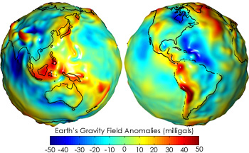
(image from https://earthobservatory.nasa.gov/features/GRACE/page3.php.) The measurement shown is the gravity “anomaly”, which is the deviation from the prediction for a smooth, uniform Earth. The unit of “milligal” is a unit of acceleration named after Galileo; one gal is equal to 0.01 m/s{}^2, which works out to about 1/1000 the size of g, so a milligal is 1/10^6 times g. Our estimated correction to g in Boulder of 0.05% of g works out to 500 milligals, so height is the dominant effect (and has clearly been subtracted to produce the shown anomaly map.)
Effective theory is a seemingly simple idea: basically an application of series expansion once again. But again, this is a really important idea in physics! Whenever we write down Newton’s laws, we’re also ignoring long-distance effects from things like the Sun’s gravitational field, and we’re ignoring quantum effects that will show up around atomic distance scales. So all of Newtonian physics is in fact an effective theory!
In fact, all of the “fundamental” forces are effective theories too, as far as we know. A famous example is gravity itself; if we try to calculate using the theory of gravity on scales where quantum mechanics is also important, then we find that the resulting effective theory diverges badly if we even ask theoretical questions about distances close to \ell_P, the Planck length I mentioned above. This is such an enormously short distance scale that we have no experiments that can possibly probe it, so far - but effective theory gives us a tantalizing hint that gravity has to change somehow if we can start to look at those really short distances.
4.6.2 Dark matter
The story of dark matter begins with a really simple physics question: how do we know the mass of the Sun M_{\odot}? I mentioned before that for the Earth, there’s only one reliable measurement of its mass, which is using the force of gravity exerted by the Earth. We can do the same for the Sun, by looking at the Earth’s orbit.
The force on the Sun due to the Earth is \vec{F}_g = -\frac{GM_{\odot} M_E}{R_{ES}^2} Now, the orbit of the Earth isn’t perfectly circular, but it’s pretty close; if we assume that it is circular, then this is also a centripetal force: \vec{F}_g = \vec{F}_c \Rightarrow \frac{GM_{\odot} M_E}{R_{ES}^2} = \frac{M_E v_E^2}{R_{ES}} or solving for the mass of the Sun, M_{\odot} = \frac{v_E^2 R_{ES}}{G}.
Finding the speed of the Earth’s orbit is easy: we know it completes a full orbit in 1 year, or 365.25 days. A full orbit is a change in angle of 2\pi, so the Earth’s angular speed is \omega_E = \frac{2\pi}{365.25\ {\textrm{days}}} \approx 2.0 \times 10^{-7} / s. Since v_E = \omega_E R_{ES}, we now know v_E in terms of R_{ES}. Determining the latter is actually tricky, although there are estimates dating back as much as 2300 years ago; I won’t go into details, but it involves geometric arguments with the Sun, Earth, and another astronomical body making a triangle. The advent of radar ranging to other planets can be combined with modern versions of these geometric calculations to yield a fairly accurate result, which I already quoted above: R_{ES} \approx 1.48 \times 10^{11} m.
Putting things together, we find M_{\odot} = \frac{\omega_E^2 R_{ES}^3}{G} = 1.9 \times 10^{30}\ {\textrm{kg}}.
For the Sun, we actually have a second way to estimate its mass: based on its size and density. Again using geometry, the radius of the Sun itself can be determined to be R_{\odot} = 7.0 \times 10^5 km. Thus, the mass will be related to the density as M_{\odot} = \rho_{\odot} V_{\odot} = \frac{4}{3} \pi R_{\odot}^3 \rho_{\odot}. We can estimate the density of the Sun because we know what it’s made of: primarily hydrogen and helium, heated into a superhot plasma. Now, this is definitely not a simple exercise: the temperature will have significant effects on the density, and so will the additional pressure generated by the huge gravitational pull of the Sun. But we have fairly complete models of the Sun’s interior, and it’s certainly possible to do the calculation carefully and get an estimate - see here for a taste of how such models work - of about 1400 kg/{\textrm{m}}^3. This once again gives a result of M_{\odot} \sim 2 \times 10^{30} kg.
This is a nice consistency check between our model of gravity and our model of the Sun. It also suggests a similar approach to a much more ambitious question: how much mass is in a galaxy like the Milky Way? The second method for weighing a galaxy is straightforward: you estimate how many stars there are, multiply by the mass of an average star (very roughly the mass of the Sun, but there are detailed models of stellar populations that can improve this!), and that gives you one version of M_{\textrm{galaxy}}.
The gravitational way of estimating a galaxy’s mass turns out to be a bit more involved. But we have a lot of extra information: since we can infer the motion of all of the visible stars in a galaxy, we can see “inside” the galaxy to probe its complete gravity field instead of having to rely only on objects well outside the galaxy, as we did for the Earth-Sun case.
Let’s restrict our attention to a certain fairly common kind of galaxy known as an elliptical galaxy, which can be nearly spherical - in fact, let’s assume it is spherical for the sake of our calculation. (I’ll comment on this assumption later.)
To find the gravitational field, we need to consider another variant of the sphere problem: finding the field inside of a solid sphere. We can set this up simply using Gauss’s law. Let’s take a sphere of radius R and consider r < R as shown:
Using the result from the tutorial, the gravitational field inside the sphere is g(r) = -\frac{4}{3}\pi G \rho r So the strength of the gravitational field actually increases with distance! We can’t observe the gravity field directly, just the motion of the stars, so we have one more step, to relate this to the speed. The main dynamics of a galaxy is not that different from our solar system: the stars follow orbits around the galactic center of mass. If we make the assumption of an approximately circular orbit, then the force of gravity must be equal to the centripetal force, |\vec{F}_g| = |\vec{F}_c| \\ m|\vec{g}(r)| = \frac{mv^2}{r} \\ \frac{4}{3} \pi G \rho r = \frac{v^2}{r} \\ v = \sqrt{\frac{4\pi G \rho}{3}} r.
We can measure v and r, and then extract the density \rho from this equation to find the galaxy mass. Of course, this is only true inside the sphere, or equivalently in the middle of the galaxy where the density really is more or less constant. But if we look at stars close to the edge of the galaxy, we can treat them as being just outside a sphere, and we have our previous result g(a) = -\frac{GM_{\textrm{enc}}}{r^2} for r > R. Relating to the speed in the same way as before, we have \frac{GM_{\textrm{enc}}}{r^2} = \frac{v^2}{r} \\ v = \sqrt{\frac{GM_{\textrm{enc}}}{r}}. So if we can get good observations of stars at the edge of a galaxy, we can just measure their speeds directly to determine the mass. Overall, if we look at all of the stars, if the density is constant out to the edge of the visible galaxy at R, we expect the profile of speed vs. distance to look like this:
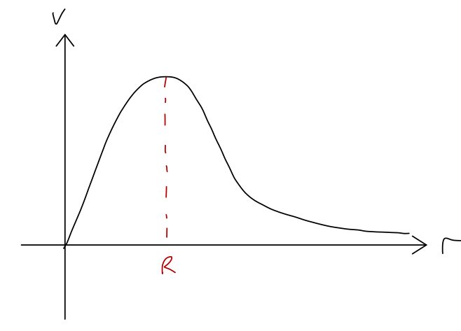
(Our prediction isn’t this smooth near R, but a smooth function is more realistic, due to measurement error and the fact that the density of a galaxy isn’t really uniform.) So far, so good. But what do we see if we actually do this experiment? Here is a plot of v vs. r for the galaxy NGC 3198: this is a spiral galaxy and not an elliptical, so I’m cheating a little; spirals seem to be easier to make this sort of observation of the full rotation curve in, probably because we get an unobstructed view of stars all the way to the center.
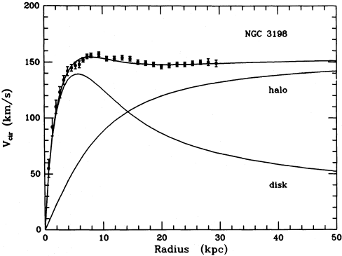
(from https://jila.colorado.edu/~ajsh/astr1200_18/dm.html, and originally https://ui.adsabs.harvard.edu/abs/1985ApJ…295..305V/abstract.)
The “disk” line shows the expected dependence; the data points show the observed results. You can see from the disk line that in this model, R for the galaxy is about 6 kpc (kilo-parsecs, a parsec is short for “parallax arcsecond” and is one of those somewhat arcane astronomy units; a parsec is about 3.3 light-years.) For small r the data agree well with the disk model, with speed increasing with distance, but then instead of the expected turnover, the velocity just becomes constant out to well beyond where the visible edge of the dense part of the galaxy is found!
One possibility is that we’ve neglected something: there is another force that we don’t know about, or our model of gravity is just wrong. This is still a possibility, although the preponderance of evidence is strongly in favor of the second option: dark matter. That is to say, what we have wrong isn’t the force law, but the density function: there must be some additional source of gravity that extends out beyond where the visible stars end. Quite far beyond, in fact; for most galaxies, a full explanation requires an enormous dark matter “halo” surrounding the visible galaxy:
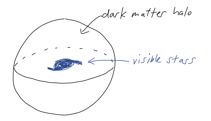
This has to be “dark” because it doesn’t emit or absorb light at all, or at best it does so very weakly; astronomical observations across the spectrum of light show nothing at all where the gravitational mass should be plentiful. This also brings me back to the comment about spherical galaxies: even for a spiral galaxy, the dark matter halo itself is still spherical (and much larger than the galaxy itself!), so our calculation still applies.
We can even guess what the density of the missing dark matter is using what we’ve derived so far: as you can see from the plot, the contribution to the speed from the halo goes roughly as \sqrt{r}. Working backwards, this requires a constant gravitational field, which in turn means that for the dark matter halo, \rho(r) \propto \frac{1}{r}. Of course, this is only one galaxy; there are other examples where v(r) becomes constant (which would require \rho(r) \propto 1/r^2) or begins to drop at very large distances. A commonly adopted model which works well for a large number of galaxies is the Navarro-Frenk-White profile, or NFW profile for short: \rho_{\textrm{NFW}}(r) = \frac{\rho_0}{(r/a)(1 + r^2/a^2)} introducing a second length scale a, the “scale radius”. This model can be argued as a simple but general parametrization of the behavior of so-called “cold and collisionless” dark matter - which can be tested using numerical simulations consisting of N masses only interacting through gravity.
Since it’s an active topic of research, I should say a little more about what we do know about dark matter. So far, the answer is “not very much”; experimental searches that attempt to capture the passing of a dark matter particle through an Earth-based detector have so far yielded nothing, except strong confirmation that it is indeed “dark” - any other interaction it has with ordinary matter must be very weak indeed.
However, we have a large amount of evidence for the gravitational effects of dark matter. In addition to observations of galactic structure (for which there are many examples):
- There is evidence for an imprint of dark matter on the cosmic microwave background, a uniform background noise that was formed in the very early universe.
- Over the very largest distance scales, the galaxies that make up our universe are not spread around randomly; instead, they seem to be organized into large, invisible filaments. This filamentary structure is consistent with simulations of the formation of the universe that include dark matter.
- Finally, according to the theory of general relativity (which replaces Newtonian gravity like special relativity replaces Newtonian mechanics), the path of a ray of light bends in a gravity field, an effect known as “gravitational lensing”. This is a complicated subject, but there are a number of observed examples where (for example) a distorted image of a distant galaxy is seen as its light passes near a closer galaxy. The mass of these lensing galaxies inferred from reconstructing the path of the light is consistent with the dark matter halo mass and not just the visible mass.
The story is not completely settled, of course; maybe a modification of gravity can account for all of the above, although since very different distances scales are involved it is quite difficult to formulate such a theory. The more likely explanation is that dark matter exists, and the hunt is on to discover what it is!