3 Momentum and conservation laws
Our next big physics topic is going to be momentum. Although we’ve sort of been ignoring it when solving problems, the concept of momentum is central to all three of Newton’s laws, and in fact the way we write the second law, \vec{F} = m \ddot{\vec{r}}, is actually not always correct! The most general correct form of Newton’s second law is the one stated in terms of momentum, \vec{F} = \dot{\vec{p}}. This is the version that applies when we extend mechanics to include special relativity. It’s also the version that applies in the case that m depends on time - the most important example of such a system is a rocket, which we’ll be studying in detail.
3.1 Conservation of linear momentum
Momentum is also a really useful concept because it obeys a conservation law, which you’ve certainly learned in intro physics and which we’ll re-derive next. The general idea of a conservation law is simple: if C is some property of a physical system, then we say that C is conserved if \frac{dC}{dt} = 0, i.e. if C doesn’t change with time. This is a simple but really powerful observation! Having a conservation law lets us do several useful things:
- If we know the starting and ending points of our system, we can calculate C_{\textrm{initial}} and C_{\textrm{final}}, and they must be equal.
- If there are parts within C that do depend on time, then setting dC/dt = 0 can give us a useful and relatively simple differential equation relating them.
- A conservation law can give us powerful qualitative insights about how different parts of a physical system interact with each other and with the outside world. For example, energy conservation means that there is no such thing as “free energy” - if a black box is producing mechanical energy, it has to be transferred from somewhere!
There is an even deeper connection between conservation laws and symmetries, which are ways in which you can change an experiment without changing the result. Probably the most important symmetry in nature, and the reason that science can work at all, is known as time translation symmetry: the fact that if you wait a little while after an experiment and then repeat it (being careful to reset the initial conditions), the outcome will be the same. It turns out that this all-important symmetry actually leads to one of the most important conservation laws, conservation of energy. Unfortunately, the framework to prove that is something you won’t see until next semester, so you’ll have to stick around to see it!
Now let’s dig into the first important conservation law we’ll discuss, conservation of linear momentum.
I’ll state it first:
For any physical system which is subject to zero net external force, the total combined linear momentum \vec{P} of all objects in that system satisfies d\vec{P}/dt = 0.
Conservation of momentum isn’t a basic, axiomatic principle; we can prove it following from Newton’s laws for a single point mass! But before we get to a proof, let’s talk about why this concept is useful. Here are a couple examples of complicated physics problems made simpler by momentum conservation:

Inelastic collisions: for example, a car crash certainly involves a lot of complicated internal forces. But momentum conservation tells us that in the absence of external forces (say, a crash on an icy road), the total momentum of both cars is conserved! Combining this with information about how the cars moved after the collision, e.g. from looking at marks left on the road, can give enough information to investigators to reconstruct the full event.
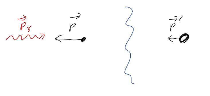
A neat special-case example of an inelastic collision is laser cooling. You’ll recall from modern physics that photons carry momentum, p = h/\lambda. Although we’ve only proved it for Newtonian mechanics, momentum conservation actually holds down to the most fundamental theories we know of! If we shine a laser on an atom at just the right frequency, the atom will absorb the photon; momentum conservation tells us that the atom has the slow down in response.
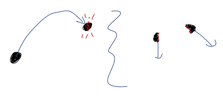
Explosions: this is basically just an inelastic collision in reverse! A firework detonation is a good example of this kind of process. Again, the internal forces involved here can be complicated and violent, but momentum conservation constrains the combined motion of all the pieces. If we track N-1 pieces after the explosion, we know exactly the trajectory of the last piece.
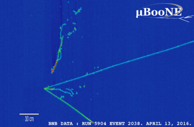
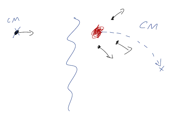
(from https://microboone-exp.fnal.gov/public/approved_plots/Event_Displays.html)
Another sub-atomic application of this sort of problem is tracking invisible particles. The picture above, from the MicroBooNE experiment at Fermilab, shows visible tracks for charged particles (like electrons) passing through their detector. However, notice that all of the tracks point back to a single point, and if we try to add up the total momentum it’s definitely pointing to the right. We can thus infer that there was an incoming particle that is invisible to our detector, which collided at the vertex where the tracks meet and caused the visible particles to fly off. (In fact, this invisible particle is a neutrino, and is precisely the particle that the MicroBooNE experiment was designed to look for!)
Now let’s run through a more quantitative example to see how this works in practice.
A hockey puck is traveling in the +\hat{x} direction at constant speed v_0 m/s. Suddenly, it breaks apart into two pieces which travel off at \theta_1 = 60^\circ and \theta_2 = 30^\circ as pictured:
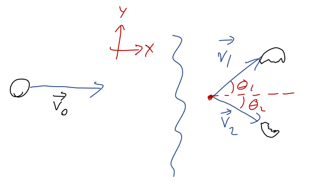
If the first piece is moving at v_1 = 4 m/s, and its mass is equal to 2/3 of the total mass of the hockey puck, what is the speed v_2 of the other piece?
Since there are no external forces, we have conservation of total momentum \vec{P}, which is most usefully written as \vec{P}_{\textrm{ initial}} = \vec{P}_{\textrm{final}}. This gives us two conservation equations, one for the \hat{x} components and one for the \hat{y} components: (m_1 + m_2) v_0 = m_1 v_1 \cos \theta_1 - m_2 v_2 \cos \theta_2 \\ 0 = m_1 v_1 \sin \theta_1 - m_2 v_2 \sin \theta_2 To relate v_2 to v_1, we can just use the second equation for the vertical components. Doing some algebra, m_1 v_1 \sin \theta_1 = m_2 v_2 \sin \theta_2 \\ v_2 = \frac{m_1 \sin \theta_1}{m_2 \sin \theta_2} v_1 If the total mass of the hockey puck is M, then since m_1 = 2M/3, we know that m_2 = M/3, since they have to add up to M. So m_1 / m_2 = 2. Plugging in \sin \theta_1 = \sqrt{3}/2 and \sin \theta_2 = 1/2, we end up with v_2 = 2 \sqrt{3} v_1 = 8 \sqrt{3}\ {\textrm{m}} / {\textrm{s}}, or about 13.8 m/s.
We only had to use conservation of momentum in the \hat{y} direction to get this far, so we still have the other equation involving P_x. We could continue and use that equation to find the only unknown quantity left, which is the speed v_0. But this won’t really be any different from the calculation we just did, so I’ll stop here.
3.1.1 Newton’s second law for extended systems
Now that we know how useful it is, let’s prove conservation of linear momentum. In fact, the conservation equation is actually just a special case of an extended version of Newton’s second law:
For a physical system consisting of multiple objects, the rate of change of total linear momentum \vec{P} is given by the net, external force \vec{F}_{\textrm{net,ext}}:
\vec{F}_{\textrm{net, ext}} = \frac{d\vec{P}}{dt}.
When \vec{F}_{\textrm{net, ext}} = 0 we find conservation of momentum, d\vec{P}/dt = 0. Our goal will be to prove this result from what we already know.
To work this out in general, we’ll say that we have a collection of N point masses, with masses m_1, m_2, ..., m_N. They can all move independently, so we’ll also have to keep track of N momentum vectors \vec{p}_1, \vec{p}_2, ..., \vec{p}_N. (Likewise there are N position vectors \vec{r}_1, ..., \vec{r}_N, but we won’t need to refer to them for present purposes.)

Let’s start by just focusing on the first two masses, 1 and 2. To be completely general, there can be forces acting between these two particles in either direction. (Our collection could be a liquid, or a solid, in which case we have bonding forces; it could be a bunch of asteroids, which would have a gravitational force; it could be a collection of electric charges…) We can divide up the net force on each object to single out that piece: \vec{F}_1 = \vec{F}_{12} + \vec{F}_{1,\textrm{ext}} \\ \vec{F}_2 = \vec{F}_{21} + \vec{F}_{2,\textrm{ext}} where \vec{F}_1 is the net force acting on mass 1, \vec{F}_{12} can be read as “the force on mass 1 by mass 2”, and \vec{F}_{1,\textrm{ext}} just represents all other forces external to the mass 1 - mass 2 system.
Now, we know that Newton’s second law will hold for each of our two masses, so \vec{F}_1 = \frac{d\vec{p}_1}{dt},\ \ \vec{F}_2 = \frac{d\vec{p}_2}{dt}. This means that if we define the total momentum \vec{P_{12}} \equiv \vec{p}_1 + \vec{p}_2, then \frac{d\vec{P}_{12}}{dt} = \vec{F}_1 + \vec{F}_2 = \vec{F}_{1,\textrm{ext}} + \vec{F}_{2,\textrm{ext}} + \vec{F}_{12} + \vec{F}_{21}. But now, we can call on Newton’s third law: the net forces between objects 1 and 2 must be equal and opposite, \vec{F}_{21} = -\vec{F}_{12}. This means that the last two terms above cancel, and we just have \frac{d\vec{P}_{12}}{dt} = \sum_{\alpha=1}^2 \vec{F}_{\alpha,\textrm{ext}} = \vec{F}_{\textrm{net, ext}}. (On the last line I used summation notation to rewrite the sum of two outside forces, and then combined them into a single net force.) So for two masses in isolation, we find that Newton’s second and third laws tell us that the combined momentum of both satisfies Newton’s second law, in terms of the outside forces acting on the pair; the momentum change due to the internal forces cancelled out in the sum.
Seeing that it works in the simple case, let’s move on to the full set of N particles. The manipulations we need to do will be similar, but we’ll have to keep track of all of the pieces. Let’s start with mass 1 again, singling out the force on it due to each other particle: \vec{F}_1 = \vec{F}_{12} + \vec{F}_{13} + ... + \vec{F}_{1N} + \vec{F}_{1,\textrm{ext}} \\ = \sum_{\alpha=2}^N \vec{F}_{1\alpha} + \vec{F}_{1,\textrm{ext}} using summation notation to write this more compactly. Similarly for the second mass, \vec{F}_2 = \sum_{\alpha \neq 2} \vec{F}_{2\alpha} + \vec{F}_{2,\textrm{ext}} where we’re adopting a new notation for the sum, which means “sum over all possible values of \alpha, except for \alpha = 2” - which is missing because mass 2 can’t exert any force on itself. (In this notation it’s implied that \alpha runs from 1 to N, instead of explicitly written on the symbol.) Seeing the pattern, we can write for an arbitrary mass \beta \vec{F}_\beta = \sum_{\alpha \neq \beta} \vec{F}_{\beta \alpha} + \vec{F}_{\beta, \textrm{ext}}. Newton’s second law tells us that \vec{F}_\beta = d\vec{p}_\beta/dt. As before, our next step is to put together the total momentum of the system, \vec{P} = \sum_\beta \vec{p}_\beta. Now we take the time derivative and apply Newton’s second law: \frac{d\vec{P}}{dt} = \sum_\beta \frac{d\vec{p}_\beta}{dt} = \sum_\beta \vec{F}_\beta \\ = \sum_\beta \left( \sum_{\alpha \neq \beta} \vec{F}_{\beta \alpha} + \vec{F}_{\beta, \textrm{ext}} \right).
Let’s continue to focus on the first “sum of sums”, the sum over all internal forces; in line with our 2-mass example, we expect this to add up to zero due to Newton’s third law. To see any cancellation happening, it can be a good idea to write things out more explicitly. Here’s what the terms in the sum look like without summation notation, excluding the \vec{F}_{\textrm{ext}} pieces: \vec{F}_{1,{\textrm{int}}} = 0 + \vec{F}_{12} + \vec{F}_{13} + ... + \vec{F}_{1N} \\ \vec{F}_{2,{\textrm{int}}} = \vec{F}_{21} + 0 + \vec{F}_{23} + ... + \vec{F}_{2N} \\ \vec{F}_{3,{\textrm{int}}} = \vec{F}_{31} + \vec{F}_{32} + 0 + ... + \vec{F}_{3N} \\ ... I’ve explicitly written zeroes in place of the ‘’missing’’ diagonal terms \vec{F}_{11}, \vec{F}_{22}... to make the pattern more obvious. For the few terms we’ve written out, we see the third-law cancellation: every \vec{F}_{\alpha \beta} has a corresponding \vec{F}_{\beta \alpha} on the opposite side of the diagonal.
The argument above is “hand-waving”, but there is a more rigorous way to prove that the double sum is zero thanks to the third law. This also shows off some useful manipulation techniques for dealing with these kinds of sums, which are nice to know for other applications (but we won’t need them again this semester.)
To show the cancellation, it should be clear that we have to split the double sum apart into pieces somehow. We can accomplish that by splitting apart the \neq sign: \sum_\beta \sum_{\alpha \neq \beta} \vec{F}_{\beta \alpha} = \sum_\beta \sum_{\alpha < \beta} \vec{F}_{\beta \alpha} + \sum_\beta \sum_{\alpha > \beta} \vec{F}_{\beta \alpha} Now, we do the following trick on the second sum: since the labels \alpha and \beta are arbitrary (like variables of integration), we can swap them. Then we notice that because the double sum means “sum over all pairs (\alpha, \beta) where \beta > \alpha”, we can invert the order of the sums and rewrite the inequality: \sum_\beta \sum_{\alpha > \beta} \vec{F}_{\beta \alpha} = \sum_\alpha \sum_{\beta > \alpha} \vec{F}_{\alpha \beta} = \sum_{\beta} \sum_{\alpha < \beta} \vec{F}_{\alpha \beta} Putting things back together gives \sum_\beta \sum_{\alpha \neq \beta} \vec{F}_{\beta \alpha} = \sum_\beta \sum_{\alpha < \beta} (\vec{F}_{\beta \alpha} + \vec{F}_{\alpha \beta}) and finally using the third law, \vec{F}_{\alpha \beta} = -\vec{F}_{\beta \alpha}, so this sum just vanishes!
If these manipulations are too arcane for you, compare back to the hand-waving argument above where I sketched out what all of the terms look like. When we divide up the sum over \alpha \neq \beta, the \alpha < \beta piece of \vec{F}_{\beta \alpha} is all the terms below the diagonal, while \alpha > \beta is the terms above. But saying “all possible \vec{F}_{\alpha \beta} where \alpha < \beta” is clearly also all the terms above the diagonal.
Thus, the double sum is just zero (since all the terms cancel!) and we have the result we wanted, \frac{d\vec{P}}{dt} = \sum_{\beta = 1}^N \vec{F}_{\beta,\textrm{ext}} = \vec{F}_{\textrm{net, ext}}.
The physics underneath the mathematics is simple: Newton’s second law for an extended system follows simply from Newton’s third law! All of the internal forces have equal-and-opposite counterparts, and so they all add up to zero when we look at the system as a whole.
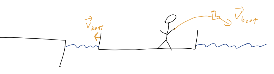
I’m standing on a boat in a completely still lake, near a dock. Everything starts at rest. If I walk at constant speed on the boat, in the direction away from the dock, how does the distance between me and the dock change?
There’s a few things to keep track of here: the boat, the dock, and me. Step one is to sketch some coordinates, then:

using subscripts for relative position, i.e. \vec{r}_{PD} is position of the person, relative to the dock. With the coordinate labels as given above, it’s clear that there is a relationship between them, namely \vec{r}_{BD} + \vec{r}_{PB} = \vec{r}_{PD}. Taking time derivatives, the same relation holds for speeds, \vec{v}_{BD} + \vec{v}_{PB} = \vec{v}_{PD}. Momentum is a different story, because for momentum the mass of each object matters. Since the dock position is fixed, the two momenta we have to keep track of are \vec{p}_{BD} = m_B \vec{v}_{BD} \\ \vec{p}_{PD} = m_P \vec{v}_{PD} and then \vec{P} = \vec{p}_{BD} + \vec{p}_{PD} for the total momentum. (Note that we don’t need to try to include the person-boat relative motion when defining \vec{P}; we’ve included all of the moving objects just with these two momentum vectors.)
Given that everything starts at rest, we know that \vec{P} = 0 at t=0. Since there are no external forces, momentum conservation thus tells us that \vec{P} is always zero. This gives us the relation \vec{P} = 0 = m_B \vec{v}_{BD} + m_P \vec{v}_{PD} \\ = m_B \vec{v}_{BD} + m_P (\vec{v}_{BD} + \vec{v}_{PB}) \\ \Rightarrow \vec{v}_{BD} = -\frac{m_P}{m_P + m_B} \vec{v}_{PB}. In other words, if the person starts walking at speed \vec{v}_0, the boat moves relative to the dock with speed given in this formula. The minus sign indicates that as we walk away from the dock, the boat moves towards it. We can also plug this in to the relation between the three velocities to find the person’s motion relative to the dock: \vec{v}_{PD} = \vec{v}_{BD} + \vec{v}_{PB} = +\frac{m_B}{m_P + m_B} \vec{v}_{PB}. It’s useful to consider the limits of m_B here. If the boat is very light, say m_B \sim m_P, then it’s very easy for our motion to influence the boat’s motion; our walking will push the boat towards the dock, and as a result we won’t move as quickly away from the dock as we would on dry land. On the other hand, if m_B \gg m_P, then \vec{v}_{BD} approaches zero while \vec{v}_{PD} \rightarrow \vec{v}_{PB}. (In other words, for a heavy enough boat, our effect on the boat’s motion is imperceptible and it’s as if we’re just walking on land.)
Just for fun, let’s plug in some numbers on a larger-scale example. The largest cruise ship in the world is the Royal Caribbean Symphony of the Seas, with a mass of about 100,000 tons, or 9 \times 10^7 kg. At maximum capacity, the Symphony can hold 7,718 people. Assuming an average person weighs about 60 kg, what would happen if everyone lined up at one end of the ship and ran to the other end at v = 5 m/s?
Treating all the people as one mass m_P = 7718 \times (60\ {\textrm{kg}}) = 4.6 \times 10^5 kg moving together, then v_{PB} is 5 m/s, and we can plug in to our formula assuming \vec{v}_{BD} = 0, i.e. the boat is initially at rest: \vec{v}_{BD} = -\frac{4.6 \times 10^5\ {\textrm{kg}}}{4.6 \times 10^5\ {\textrm{kg}} + 9 \times 10^7\ {\textrm{kg}}} (+5\ {\textrm{m}}/{\textrm{s}}) = 0.025\ {\textrm{m}}/{\textrm{s}} or 0.06 mph. So I don’t think anything noticeable will happen to the ship - it’s simply too heavy! (On the other hand, if you’ve been on a small few-person boat on a lake, you know that your own movements can have a significant effect on how the boat moves.)
3.2 Rockets
For a compound system, as we’ve seen, we can change the momentum of one part of the system by causing some motion to happen to another part. In our boat example problem, the person can actually move the entire boat just by walking across it in the opposite direction. However, there are practical limits in that case: the person can only walk so far, and as we saw the distance from person to dock always increases in that example - so you can’t use this trick to make it back to dry land if your motor shuts off.
A better way to exploit conservation of momentum in the boat example is by using projectiles. If you take an object on the boat and throw it overboard, conservation of momentum requires that the boat will be pushed forward in the opposite direction. Since the object is separated from the boat, we can get closer to dry land in this way - the only practical limit is how many things we have to throw in order to propel ourselves forwards.
This is, in fact, an example of rocket propulsion: the idea of propelling a vessel forwards by ejecting part of its mass in the opposite direction that we want to travel. If we consider the vessel and the ejected mass to be part of the same system, there are only internal forces active, so we have d\vec{P}/dt = 0. Of course, throwing things by hand isn’t very efficient; when I say the word “rocket”, you probably picture something that uses a chemical reaction to eject super-hot gas.
Before we get to this kind of rocket (which requires dealing with a continuous rate of mass ejection), let’s consider a detailed example of the simpler kind of rocket propulsion on the next tutorial.
Here, you should complete Tutorial 3A on “Momentum conservation and rockets”. (Tutorials are not included with these lecture notes; if you’re in the class, you will find them on Canvas.)
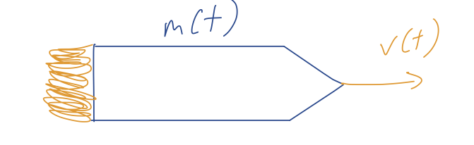
Now that we’ve built some intuition, let’s do the case of continuous mass ejection. We’ll assume our rocket is continuously ejecting mass at a rate dm/dt, so the rocket itself has a mass-dependent time m(t). The speed at which the mass is ejected, called the exhaust speed v_{\textrm{exh}}, is also important. To begin with, we’ll assume all external forces are zero; it will be easy to generalize.
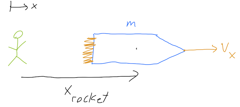
Let’s work more carefully, which means starting with an inertial frame of reference (the rocket will accelerate, so its frame is no good.) What does an observer on the ground see, watching the rocket system? Let’s set up some coordinates, considering both the rocket and an infinitesmal bit of mass dm being ejected, and just considering motion in a single direction x:
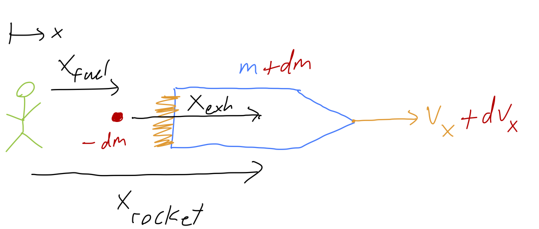
Just like the boat example, x_{\textrm{exh}} = x_{\textrm{rocket}} - x_{\textrm{fuel}} is a redundant but useful coordinate describing the position of the bit of fuel dm relative to the rocket. Notice that we’re writing the mass of the fuel as “-dm”, which means dm itself is negative: this will give us dm/dt < 0 for the rocket itself, which it has to be since it’s losing mass. (This is a little confusing here, but less confusing later!)
Using these coordinates, we can derive the relationship between the velocity of the fuel and the velocity of the rocket: v_{x,\textrm{exh}} + v_{x,\textrm{fuel}} = v_{x,\textrm{rocket}} \\ v_{x,\textrm{exh}} + v_{x,\textrm{fuel}} = v_{x,\textrm{rocket}} \\ v_{x,\textrm{fuel}} = -v_{x,\textrm{exh}} + v_{x,\textrm{rocket}}.
Note that I’m writing out the x subscripts explicitly mid-derivation, to remind us that we’re working with v_x \equiv dx/dt, which is a component of velocity and NOT a speed - it can be positive or negative!
Let’s be extra careful about that second term. The fuel is being ejected backwards from the rocket, so we might be tempted to say that v_{x,\textrm{exh}} is negative. But if we look at our diagram, the fuel is moving away from the rocket, which means x_{\textrm{exh}} is increasing. Therefore, v_{x,\textrm{exh}} = |v_{\textrm{exh}}| is positive! (This is, basically, because we drew our arrow from the fuel to the rocket; so the positive v_{x,\textrm{exh}} is the velocity of the rocket moving away from the fuel, basically.)
Here I’m writing |v_{\textrm{exh}}| with an absolute value sign to make it completely clear that it is a speed (i.e., always positive - this matches Taylor’s conventions, although he omits the absolute value sign.) Plugging in to our equation above, then, we have the relationship v_{x,\textrm{fuel}} = -|v_{\textrm{exh}}| + (v_x + dv_x).
Before we continue, let’s do a couple of checks:
What happens if the rocket starts from rest, v = 0? Ignoring the tiny change dv, we can plug in to our formula above to see that v_{x,\textrm{fuel}} = -|v_{\textrm{exh}}|. This answer makes sense; with v=0 now there is no difference between the perspective of the rocket and the observer (since they’re at relative rest), and they agree that the fuel is just coming out at the exhaust speed, to the left.
What happens if the rocket is moving at the exhaust speed, v = |v_{\textrm{exh}}|? Using the formula again, we simply have v_{x,\textrm{fuel}} = 0. Now the fuel looks like it’s at rest when ejected, according to the ground observer. This also makes sense (convince yourself!)
Moving on, we can apply conservation of momentum: \vec{P}(t) = \vec{P}(t+dt) \\ mv_x = p_{\textrm{fuel}} + p_{\textrm{rocket}} \\ = (-dm) v_{x,\textrm{fuel}} + (m+dm) (v_x + dv_x) Cancelling off the mv_x on both sides, this becomes 0 = (-dm) (-|v_{\textrm{exh}}| + v_x + dv_x) + v_x dm + m dv_x \\ -|v_{\textrm{exh}}| dm = m dv_x where a couple more cancellations have happened. Finally, to get a differential equation we restore the time differential dt: m \frac{dv_x}{dt} = -|v_{\textrm{exh}}| \frac{dm}{dt}. This is the rocket equation, which will let us calculate the motion of the rocket. Remember, the rocket is losing mass, so dm/dt < 0, which means that dv_x/dt > 0, i.e. the rocket moves forwards. Since this ends up looking exactly like Newton’s second law, we can identify the right-hand side as a force, called the thrust:
The thrust force of a rocket with exhaust speed |v_{\textrm{exh}}| and mass ejection rate dm/dt < 0 is equal to:
F_{\textrm{thrust}} = -|v_{\textrm{exh}}| \frac{dm}{dt}.
For a rocket to achieve larger thrust, we see that either the reaction has to be faster (so |dm/dt| goes up), or more energetic (so |v_{\textrm{exh}}| goes up.)
In general, we could have a rocket where the exhaust speed is a function of time. However, if it is constant, we can easily integrate to find the motion - let’s do an example.
Suppose we have a rocket-powered car moving in a straight line across a flat surface. Ignoring friction and air resistance, how does the position of the car change with time?
As always we start with the equation of motion, which is m(t) \ddot{x} = F_{\textrm{thrust}}.
This looks simple, but we have to deal with the extra complication that m(t) is time dependent. Fortunately, since we know that the mass ejection rate is constant, it’s easy to see that m(t) = m_0 - kt. Our equation of motion is nice and separable: moving things around and integrating, we find first that \int_{\dot{x}(0)}^{\dot{x}(t)} d\dot{x}' = F_{\textrm{thrust}} \int_0^t \frac{dt'}{m_0 - kt'} \\ \dot{x}(t) = \dot{x}(0) - \frac{F_{\textrm{thrust}}}{k} \ln \left(1 - \frac{kt}{m_0}\right). To get the position, we integrate one more time. A useful identity is \int dx \ln x = x \ln x - x (which you can easily check by taking the derivative!) Applying this to our result above, we see that (using u = 1 - (kt/m_0)) \int dt\ \ln \left(1 - \frac{kt}{m_0} \right) = -\frac{m_0}{k} \int du \ln u \\ = -\frac{m_0}{k} (u \ln u - u) \\ = \left(\frac{m_0}{k} - t\right) \left[1 - \ln \left( 1 - \frac{kt}{m_0} \right) \right]
Plugging back in, we end up with x(t) = x(0) + \left(\dot{x}(0) + \frac{F_{\textrm{thrust}}}{k} \right) t + \frac{F_{\textrm{thrust}} (m_0 - kt)}{k^2} \ln \left(1 - \frac{kt}{m_0}\right).
This is an analytic solution, but it’s already pretty complicated - and this was the simplest possible case, with no other forces acting! It’s also worth noting that this solution is not valid for all times: mathematically, we can see that at t = m_0 / k the log blows up, and we have x(m_0 / k) \rightarrow \infty!
Of course, t = m_0 / k is the time at which m(t) = 0, which is obviously not possible. Physically, we know that our solution is only valid until the fuel is burned completely, at which point F_{\textrm{thrust}} shuts off and we just have constant speed from that point on (the speed we already found with the rocket equation above, in fact.)
3.2.1 Rocket speed vs. mass
There’s one more useful way to think about rockets, starting from the version of the rocket equation before we introduced the dt: -\frac{dv_x}{|v_{\textrm{exh}}|} = \frac{dm}{m} \\ v_x(m) = -|v_{\textrm{exh}}| \ln m + C Using the generic initial condition that v_x(m_0) = v_0, we have C = v_0 + |v_{\textrm{exh}}| \ln m_0 \\ \Rightarrow v_x(m) = v_0 + |v_{\textrm{exh}}| \ln (m_0/m).
Since this relates v_x to m directly, this is true whether or not dm/dt is constant (!) (If dm/dt is constant, then we have constant thrust and we can just find m(t) and then integrate with respect to time.)
The bad news in this equation is that we have a logarithmic dependence on mass - this makes it very difficult to increase the top speed of our rocket by just adding more fuel! To be concrete, we can write m_0 = m_E + m_F where m_E is the mass of the empty rocket, and m_F is the mass of the fuel. (If you’re looking up real-world information on rockets, m_E is often called the “dry mass”, while the total m_E + m_F including the fuel is the “wet mass”.) Then the top speed of the rocket, if it starts from rest, is v_{\textrm{max}} = v(m_E) = |v_{\textrm{exh}}| \ln \left( 1 + \frac{m_F}{m_E} \right) So if the exhaust velocity is fixed, just making our rocket bigger alone won’t help; if we double the size of the rocket and both m_E and m_F are twice as large, the top speed doesn’t increase at all! We need to either increase m_F without making the rocket heavier, or make m_E lighter with the same amount of fuel.
Even if we can accomplish those engineering feats, the gains are heavily diminishing. Suppose we build a rocket which has 90% of its mass devoted to fuel, so m_F = 10 m_E. Then its top speed is about 2.4 times |v_{\textrm{exh}}|. If we somehow strip nearly all the mass out of the rocket and make a better design which is 99% fuel by mass, then m_F = 100 m_E, but the top speed will only go up to 4.6 times |v_{\textrm{exh}}|. Physically, it’s easy to see the problem: to get more total thrust we need more mass to eject, but if we start with more mass, then we get less speed for the same amount of thrust.
What if we have other external forces? If we wanted to track the motion of the rocket-exhaust system combined, we could keep track of the combined center of mass and see how the forces act on that. However, this would be complicated to do! Fortunately, we don’t care about the combined system - we only care about the net forces on the rocket itself. So if we have additional forces like drag or gravity, we just treat them as acting on the rocket, in addition to the thrust force provided by the ejected mass.
For example, taking both forces above at once and assuming quadratic drag, a rocket moving vertically from the Earth’s surface has the equation of motion m(t) \dot{v}_y = \vec{F}_{\textrm{thrust}} - m(t) g - cv_y^2. although this will get more complicated quickly if we remember that the density of air depends strongly on altitude, so c = c(z) for a more realistic model (and at some point, g starts to change too, and so on.) This also means there’s no terminal velocity for a rocket launch into space; once it gets out of the Earth’s atmosphere and away from the Earth’s gravity, the rocket will just continue to move at constant speed.
As you can start to see, getting much further with practical examples of rocketry is going to require a lot of additional details, and the equations will become difficult to handle very, very quickly. Basically, any realistic rocket problems are going to involve heavy use of numerical solutions. The main interesting exception is a multi-stage rocket, but I’ll include that as a bonus example since there is not really any new physics compared to a simple rocket - just a bit more complication.
A multi-stage rocket is just multiple rockets, stuck together. The rockets are burned one at a time, with the spent rockets being ejected after they are used up. For example, in a two-stage rocket the first stage is burned, then ejected, so that the second stage only has to propel itself and the cargo from that point:

Ignoring all other forces (e.g. imagine we’re working in deep space), let’s compare the maximum speed of two different rockets. Rocket A is simple rocket with a fuel-to-mass ratio of m_{A,F} / m_{A,E} = 25. Rocket B is a two-stage rocket, which means it’s two rockets stuck together: both stage 1 and stage 2 have a fuel-to-mass ratio of m_{B1,F} / m_{B1,E} = m_{B2,F} / m_{B2,E} = 10. Stage 2 is also about 5 times lighter than stage 1, i.e. m_{B1,E} / m_{B2,E} = 5. Assuming v_{\textrm{exh}} = 2.5 km/s, what is the \Delta v supplied by each rocket?
We only need one equation here, although we’ll need it a few times. From above, we can get the \Delta v for rocket A just by plugging in: (\Delta v)_A = |v_{\textrm{exh}}| \log \left(1 + \frac{m_{A,F}}{m_{A,E}} \right) \\ = |v_{\textrm{exh}}| \log \left(1 + 25 \right) = 8.1\ {\textrm{km}} / {\textrm{s}}
For the two-stage rocket, we have to be more careful what masses we plug in. Let’s working in units of the mass of the empty second stage, m_{B2,E} \equiv m, since this is the lightest mass in the problem. In these units, we have for example the empty first stage m_{B1,E} = 5m.
Let’s now work through the first-stage burn, finding the appropriate m_E and m_F to use with our formula. Since the fuel-to-mass ratios for both of the two stages are 10, we have m_{B2, F} = 10m and m_{B1,F} = 50m. For the first stage, only the mass of the burned fuel matters. So m_F = 50m, the fuel in the first stage alone. For the “empty” mass, however, we need to be more careful: the “empty” first stage includes the mass of the second stage, which is being carried as cargo! This includes the second-stage fuel, which hasn’t been burned yet. Thus, the mass after the burn is m_E = m_{B1,E} + m_{B2,F} + m_{B2,E} = 5m + 10m + m = 16m.
So after the first-stage burn, we have (\Delta v)_{B1} = |v_{\textrm{exh}}| \log \left(1 + \frac{50}{16} \right) = 3.5\ {\textrm{km}} / {\textrm{s}} Now we discard the first stage and just consider the second stage alone, which is much easier to plug in for: (\Delta v)_{B2} = |v_{\textrm{exh}}| \log \left(1 + 10\right) = 6.0\ {\textrm{km}} / {\textrm{s}} So in total, the second rocket achieves (\Delta v)_B = 9.5\ {\textrm{km}}/{\textrm{s}}, somewhat better than rocket A - despite the fact that the individual stages had a much lower fuel-to-mass ratio! Qualitatively, this makes sense: if we can dump some of the mass of our rocket partway through, then the fuel-to-mass ratio at that point is immediately improved. (After the first-stage burn but before separation, our fuel-to-mass ratio is all the way down to 1.7.)
By the way, 25 to 1 is generally considered about the best possible ratio for a single rocket stage, based on available technology for both rocket fuels and engineering the rocket itself. The ratio of 5 in mass between the two stages is taken from SpaceX’s Falcon 9 rocket, but the real Falcon 9 has much better single-stage performance, with 18:1 for the first stage and 25:1 for the second. This gives the Falcon 9 an approximate \Delta v of 12.1 km/s (before including a payload) - large enough that we can start thinking about escaping the Earth completely and going elsewhere in the Solar system (like Mars!)
3.3 Center of mass
Going back to our extended system of N point masses, let’s now think about their positions \vec{r}_1, ..., \vec{r}_N. Since the momentum of a point mass is \vec{p}_\alpha = m_\alpha \dot{\vec{r}}_\alpha, we can actually rewrite the total momentum in terms of individual speeds, \vec{P} = \sum_\alpha \vec{p}_\alpha = \sum_\alpha m_\alpha \dot{\vec{r}}_\beta. Just based on dimensions, if we divide \vec{P} by a mass scale, we’ll get a velocity vector of some sort. Since this is the total momentum, it makes the most sense to divide by the total mass: if M = \sum_\beta m_\beta then we define the total velocity vector to be \vec{V} = \frac{\vec{P}}{M} = \frac{1}{M} \sum_{\alpha=1}^N m_\alpha \dot{\vec{r}}_\alpha. Looking at the definition, this is just the time derivative of another vector, which we’ll call the center of mass (or “CM”) position vector: \vec{V} = \dot{\vec{R}},\ \ \vec{R} = \frac{1}{M} \sum_{\alpha=1}^N m_\alpha \vec{r}_\alpha. Some references will write this as \vec{R}_{CM} to be explicit; I’ll skip the subscript as long as it’s clear from context. The CM vector \vec{R} gives sort of a weighted average of the positions of all the objects in our system, with weighting proportional to their mass. And now we notice that if we go back to the equation for external net force, we find \frac{d\vec{P}}{dt} = M \ddot{\vec{R}} = \vec{F}_{\textrm{net, ext}}. So the center of mass position evolves like a point particle with total mass M, following Newton’s second law and subject to the net external force acting on the system. This immediately justifies a common approximation used in mechanics, which is that we can treat large, extended objects the same way we treat point particles when applying Newton’s laws.
3.3.1 Center of mass and symmetry
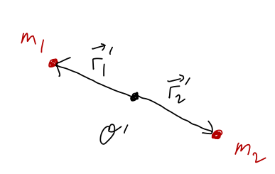
Before we get into doing any integrals, it’s a good idea to run through the center of mass calculation for two point masses, which we’ll call m_1 and m_2. Let’s set up our coordinates like this:

Using our formulas above, we have \vec{R} = \frac{m_1}{m_1 + m_2} \vec{r}_1 + \frac{m_2}{m_1 + m_2} \vec{r}_2 Notice that if we take m_1 \rightarrow 0, then the CM position approaches \vec{R} = \vec{r}_2, and vice-versa. So the CM position tends to be closest to the heavier mass. On the other hand, if m_1 = m_2, then \vec{R} = \frac{1}{2}(\vec{r}_1 + \vec{r}_2) which is exactly in the center between the masses.
We can make a couple more nice observations in the two-mass case by changing coordinates. First, let’s try setting \vec{r}_1 = 0, i.e. putting mass 1 at the origin of our coordinates. Then we have \vec{R} \rightarrow \frac{m_2}{m_1 + m_2} \vec{r}_2 so \vec{R} points in the same direction as \vec{r}_2. In other words, the position of the center of mass is along the line between m_1 and m_2.
Finally, let’s put our coordinate origin at the geometric center, exactly halfway in between \vec{r}_1 and \vec{r}_2 as shown:
Measured from this point, we have \vec{r}'_2 = -\vec{r}'_1. Using this relation in the general formula gives \vec{R} = \frac{m_1}{m_1 + m_2} \vec{r}'_1 - \frac{m_2}{m_1 + m_2} \vec{r}'_1 In general, the CM is not at the geometric center; it will be closer to the heavier mass out of m_1 or m_2. However, in the special case where m_1 = m_2, the two terms are equal and opposite and cancel completely. The situation where this cancellation happens is said to exhibit reflection symmetry or mirror symmetry about the origin; mirror reflection takes \vec{r} \rightarrow -\vec{r}, so with \vec{r}'_2 = -\vec{r}'_1 we can think of mass 2 as a ‘reflection’ of mass 1 if they are identical.
This probably seems like a really special case, but notice what happens if we add two more masses along a different line:
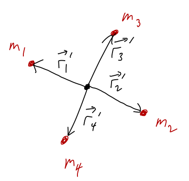
With \vec{r}'_4 = -\vec{r}'_3, we have \vec{R} = \frac{m_1 - m_2}{M} \vec{r}'_1 + \frac{m_3 - m_4}{M} \vec{r}'_3 and once again, if the pairs (m_1, m_2) and (m_3, m_4) are reflection symmetric, then both pairs contribute zero to the CM position and we find \vec{R} = 0.
What we’re seeing is a very general and powerful rule that applies to calculating the center of mass: if we have two equal masses m_1 = m_2 at exactly opposite positions, \vec{r}_1 = -\vec{r}_2, then their total contribution to the CM is zero.
3.3.2 Finding the center of mass
Of course, most everyday objects are pretty complicated, and in fact even a tennis ball is made of an incredible large number of individual tennis-ball particles. For situations where N would be very large, we can instead replace the sum with an integral. (Think back to your calculus class - this is how integrals are originally defined!)
For the situation where N is very large, we can replace the discrete set of point masses \{ m_\alpha \} with a continuous set of infinitesmal masses dm. (Notation aside: curly brackets is math notation for a set, which is a collection of mathematical objects. m_\alpha denotes one point mass; \{ m_\alpha \} is the collection of all of them.) Since each tiny speck of mass has its own position, we have to define a function of position \vec{r} to keep track of them. We define the mass density function \rho(\vec{r}) through the relationship dm = \rho(\vec{r})\ dV By inspection \rho(r) has units of mass per unit volume, [M]/[L]^3. With this definition, all of the sums over masses become integrals over dm:
For an extended object with mass density \rho(\vec{r}), the position \vec{R} of its center of mass is \vec{R} = \frac{1}{M} \int \vec{r}\ dm = \frac{1}{M} \int \rho(\vec{r}) \vec{r}\ dV, where the total mass M is given by M = \int dm = \int \rho(\vec{r}) dV.
We could write similar formulas for \vec{P} and \vec{V}, but they’re easily obtained by just taking derivatives of \vec{R}.
Don’t get confused by the fact that we’re integrating over a vector! Since both sides of the equation are vectors, this is really just three separate integrals for each of the components, i.e. in Cartesian components X_{CM} = \frac{1}{M} \int x\ dm,\ \ Y_{CM} = \frac{1}{M} \int y\ dm,\ \ Z_{CM} = \frac{1}{M} \int z\ dm. The components are almost always found in Cartesian components, even if the integrals themselves are easier to do in cylindrical, spherical, etc. coordinates.
Before we move on to examples, one comment about the definition of dm. The replacement we’ve used above is only really appropriate for three-dimensional objects, for which it makes sense to talk about the “volume” of the object. But we’ll see a number of examples where we’re interested in objects that don’t really have volume, because they’re flat (two-dimensional) or thin lines (one-dimensional.) We can handle these various cases by adjusting the form of dm:
dm = \rho(\vec{r}) dV (solid object, 3-d)
dm = \sigma(\vec{r}) dA (flat object, 2-d)
dm = \lambda(\vec{r}) ds (linear object, 1-d)
Here \rho, \sigma, \lambda are all forms of “density”, but with different units, for example \sigma (the “area density”) has units of kg / m{}^2, while \lambda (the “linear density”) has units of kg / m.
Of course, we live in three dimensions so there is no such thing as a truly flat object - these are just approximations. In fact, we can understand a bit better how these definitions are related if we imagine working with a real “flat” object, say a rectangular prism which is square on two sides with side length a, and then has a thickness b \ll a in the third dimension. The total mass of the disk will be, using cylindrical coordinates:
M = \int dm = \int_0^a dx \int_0^a dy \int_{0}^{b} dz\ \rho(x,y,z) If we assume that b is so tiny that the difference between \rho(x,y,b) and \rho(x,y,0) is negligible, then we can just do the z-integral assuming the density is constant in that direction:
M \approx \int_0^a dx \int_0^a dy \left[ b \rho(x,y,0) \right] \equiv \int_0^a dx \int_0^a dy\ \sigma(x,y). In other words, integrating over the infinitesmally thin z-direction gives us the combination of thickness times volume density, which we can just rewrite and think about as an area density.
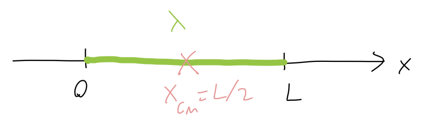
As a warm-up to more interesting continuous objects, let’s compute the center of mass of a rod of length L, which we will assume is very thin (so its other two dimensions are negligible.)

Since this object is (effectively) one-dimensional, we can treat it using a linear mass density, and we only have to worry about the x-direction. So, for the center of mass position we have the single integral X_{CM} = \frac{1}{M} \int x dm = \frac{1}{M} \int_0^L dx\ x \lambda(x) (identifying ds = dx since the rod is along the x-axis) and then, for the total mass, M = \int dm = \int_0^L dx\ \lambda(x).
Now, if the rod has constant density \lambda(x) = \lambda = M/L, then we have a simple symmetry argument that the CM position is at X_{CM} = L/2: for any point we pick on one side of the rod, there is an equal point reflected across L/2 with the same mass.
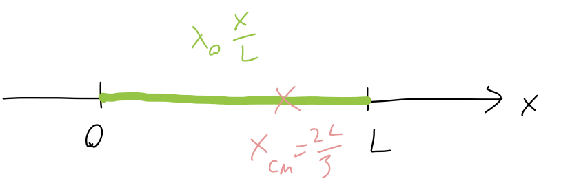
Things become more interesting if the linear density is not constant anymore. Let’s take a linear density: \lambda(x) = \frac{\lambda_0}{L} x. (This isn’t very realistic since the density goes all the way to zero at x=0, but it’s mathematically simple.) Now the symmetry argument fails, since the reflected points will have different masses. In fact, since the mass density increases with x, we can anticipate before we do any more math that X_{CM} > L/2, since the mass is concentrated more towards the end of the rod at x=L.
Let’s do the math: first, with this density, the total mass is M = \int_0^L dx\ \frac{\lambda_0}{L} x \\ = \frac{\lambda_0}{L} \left.\frac{1}{2} x^2 \right|_0^L \\ = \frac{1}{2} \lambda_0 L. or, rearranging a bit, \lambda_0 = \frac{2M}{L}.
Then for the center of mass: X_{CM} = \frac{1}{M} \int_0^L dx\ x \frac{\lambda_0}{L} x \\ = \frac{\lambda_0}{ML} \frac{1}{3} L^3 \\ = \frac{2M}{ML} \frac{1}{3} L^2 \\ = \frac{2}{3} L.
So indeed, the CM is shifted towards the heavier side as we guessed.
Now that we’re warmed up, let’s move up to two dimensions with a tutorial!
Here, you should complete Tutorial 3B on “Center of mass”. (Tutorials are not included with these lecture notes; if you’re in the class, you will find them on Canvas.)
Finally, on to a three-dimensional example.
In this example we will find the center of mass for a cylinder of uniform density:
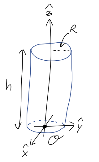
Let’s just set up and do the integrals, and then we’ll think about the results. With uniform (i.e. constant) density, we have simply \rho(\vec{r}) = \rho. We put the origin at the center of the bottom of the cylinder, as shown. Starting with the x-position: X_{CM} = \frac{1}{M} \int x\ dm = \frac{1}{M} \int x (\rho\ dV) = \frac{\rho}{M} \int_0^{2\pi} d\phi \int_0^R dr \int_0^h dz\ r x using cylindrical coordinates to expand out dV, which gives us a factor of r. (I am also using r instead of \rho for the cylindrical radius, because we have another \rho already, the density!) Thinking back to the definition of cylindrical coordinates, we recall that x = r \cos \phi, so the integrand is r^2 \cos \phi. All of the integrals are separate and easy to do, but let me go slowly and do them in order for this first example: X_{CM} = \frac{\rho}{M} \int_0^{2\pi} d\phi \int_0^R dr\ r^2 \cos \phi \left.(z) \right|_0^h \\ = \frac{\rho}{M} h \int_0^{2\pi} d\phi\ \cos \phi \left. \left( \frac{1}{3} r^3 \right) \right|_0^R \\ = \frac{\rho}{3M} h R^3 \left. (\sin \phi) \right|_0^{2\pi} \\ = \frac{\rho}{3M} h R^3 (\sin 2\pi - \sin 0) = 0 So we just have X_{CM} = 0. I’ll leave it as a short exercise to convince yourself that similarly, Y_{CM} ends up proportional to \cos 2\pi - \cos 0, so that also Y_{CM} = 0. Finally, for the z position, we have Z_{CM} = \frac{\rho}{M} \int_0^{2\pi} d\phi \int_0^R dr \int_0^h dz\ r z \\ = \frac{2\pi \rho}{M} \left(\frac{1}{2} h^2\right) \left( \frac{1}{2} R^2 \right) = \frac{\pi \rho h^2 R^2}{2M}. To simplify further, we recognize that \rho and M are related to each other. For constant density we just have M = \rho V, but I’ll just do the integral: M = \int \rho dm = \int_0^{2\pi} d\phi \int_0^R dr \int_0^h dz\ \rho r = \pi R^2 h \rho. Plugging back in then gives us the much simpler result Z_{CM} = \frac{h}{2}.
Gathering our results, the center of mass of the cylinder (in the chosen coordinates) is at \vec{R} = (0, 0, h/2). This is also the geometric center of the cylinder.
Zero is a pretty special result, so let’s go back and think about why we found that for X_{CM} and Y_{CM} in the example above. Before we convert to cylindrical coordinates, the integral for X_{CM} can be written in the form: X_{CM} = \frac{\rho}{M} \int_{-R}^R dx\ x \int dy \int dz = \frac{\rho}{M} \int_{-R}^R dx\ x f(x) where f(x) is the result of doing the y and z integrals out first. We get a function of x because the y limits of integration depend on x. (The function f(x) isn’t too difficult to find explicitly, and if you need practice with integrating go ahead and try it!) All we need to know is that f(x) is reflection symmetric, f(-x) = f(x). This has to be true because if we reflect the cylinder along the x-axis about the origin, it looks completely identical. (I say “reflect along the x-axis”, but really what this means is you should imagine a plane perpendicular to the x-axis and containing the origin. That plane is acting like a mirror for the reflection.)
Knowing this one geometric fact, we have X_{CM} \propto \int_{-R}^R dx\ x f(x) = \int_{-R}^0 dx\ x f(x) + \int_0^R dx\ x f(x) \\ = \int_R^0 (-dx) (-x) f(-x) + \int_0^R dx\ x f(x) \\ = -\int_0^R dx\ x f(x) + \int_0^R dx\ x f(x) = 0. (the symbol \propto means “is proportional to”, i.e. ignoring the \rho/M out front.) Similarly, the fact that the cylinder is identical if we reflect along the \hat{y}-axis lets us predict immediately that Y_{CM} = 0, even before we actually do the integral. This doesn’t work for the \hat{z} direction, because if we reflect about the origin, (i.e. through a plane containing the origin and perpendicular to \hat{z}), our sketch looks different:
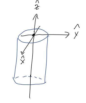
On the other hand, if we put the origin halfway up the cylinder’s axis at z=h/2, then we have the reflection symmetry and would find Z_{CM} = 0 - exactly in agreement with our third result above. In math terms, this is the difference between integrating from 0 to h and from -h/2 to h/2 - we need the symmetric interval of integration for the two halves of the integral to cancel off.
There’s a more physical explanation for why the mathematics works out this way; it’s exactly the same cancellation that we saw before in our point-mass examples. Because of the reflection symmetry in the \hat{x} direction, for any little bit of mass dm that we identify in the cylinder, there is a corresponding (and identical) bit of mass dm on the other side of the origin. As we saw above, the contribution of these two masses to the CM location will balance and cancel off.
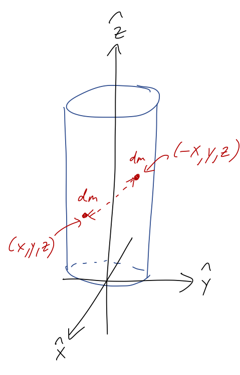
Likewise, we see that reflecting about the CM at Z_{CM} = h/2, the mass on either side in the \hat{z} direction is perfectly balanced. We could have used this observation to see that Z_{CM} = h/2, again without having to actually do any integrals. Symmetry is powerful!
Now suppose we have a half-cylinder, cut in half through the circular direction as shown:
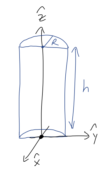
What is the CM position?
Answer:
Let’s begin with Y_{CM} and Z_{CM}; for these two directions, we can use symmetry to find the answer without doing any math! In the \hat{y} direction, we notice that we have reflection symmetry about the axis through the middle of the half-cylinder: every point (x,y,z) in the cylinder has a matching point at (x,-y,z). So Y_{CM} = 0 by symmetry.
Similarly, in the \hat{z} direction we still have reflection symmetry about the plane halfway through the half-cylinder, so Z_{CM} = h/2 as in the previous case.
We can’t apply these arguments to X_{CM}, because there’s nowhere that we can put a mirror perpendicular to \hat{x} that will reflect our object without giving a different image! So symmetry helped us twice, but we have to do one integral. Let’s set it up: we have X_{CM} = \frac{1}{M} \int \rho\ x\ dV \\ = \frac{\rho}{M} \int_0^\pi d\phi \int_0^R r dr \int_0^h dz (r \cos \phi) where the only adjustment we need to make for the half-cylinder is that our polar angle runs from \pi/2 to 3\pi/2 (look carefully at the diagram!) Doing the integrals gives X_{CM} = \frac{\rho}{M} \left.\frac{hR^3}{3} (\sin \phi) \right|_{\pi/2}^{3\pi/2} \\ = -\frac{2hR^3\rho}{3M} (the minus sign puts it inside the half-cylinder according to our chosen coordinates, which makes sense.) Since this is a half-cylinder, its volume is just half of the standard volume, V = (1/2) \pi R^2 h, which means M = \frac{1}{2} \pi R^2 h \rho allowing us to simplify the answer to X_{CM} = -\frac{4R}{3\pi}. which is about -0.4 times R - not quite halfway up the semicircle, which makes sense since there’s more mass around x=0 than x=R. (This is very similar to the example of the hemisphere we just considered.)3.3.3 Using the center of mass
Now that we have a good idea of how to find the CM, we should step back for a moment and reflect on why it’s useful to find the CM. Formally, the CM is a useful idea because if we only have external forces pushing a large object around, we can treat the whole thing as a point particle located at the CM. There are a few more specific implications of this fact:
Explosion and collision problems: Since the CM position obeys Newton’s second law with respect to external forces, \vec{F}_{\textrm{ext}} = m \ddot{\vec{R}}, we know that for processes with just internal forces, like an explosion, the CM will move as if no forces at all are acting upon it! (More realistically, we usually have at least gravity. For an object exploding in mid-air, for example, the CM of the pieces will continue to move as a simple free-falling point mass, even after the explosion!) Using the CM can give a more economical way to deal with such momentum-conservation problems.
Recall the broken hockey puck example from above:
The problem we solved with momentum conservation was: given that v_1 = 4 m/s and the angles are \theta_1 = 60^\circ and \theta_2 = 30^\circ, what is v_2? We can think of this in terms of the CM instead: because there are no external forces, the CM must continue moving along the \hat{x}-axis at speed v_0 even after the puck breaks apart. Since the CM position is \vec{R} = \frac{1}{M} (m_1 \vec{r}_1 + m_2 \vec{r}_2) = \frac{2}{3} \vec{r}_1 + \frac{1}{3} \vec{r}_2, we can just take a time derivative of both sides to get \dot{\vec{R}} = \vec{v}_0 = \frac{2}{3} \vec{v}_1 + \frac{1}{3} \vec{v}_2 \\ (v_0, 0) = \frac{2}{3} (v_1 \cos \theta_1, v_1 \sin \theta_1) + \frac{1}{3} (v_2 \cos \theta_2, -v_2 \sin \theta_2) These are the same equations we found through conservation of momentum (they had to be!), but we arrived at them a bit faster. This approach of using the CM position directly for explosion and collision problems is usually an even better shortcut if the object in question breaks into more than two pieces.
Balancing forces: One of the more well-known properties of the CM is that an object can be balanced even on a point, so long that CM is directly above the balance point. We can sketch the gravity and normal forces as follows:
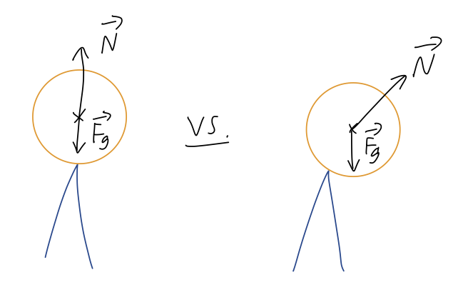
Gravity always acts straight down on the CM, but the normal force direction is always perpendicular to the contact between the surfaces. So if our object is tipped over slightly, the normal force will no longer balance against gravity completely, and the net force will cause the object to tip further.
You might ask: what if I had a completely flat object balanced on a thin rod? Once again, our flat object will tip over unless the rod is placed directly below the CM. But in this case, it seems like the normal force is always straight up, so why is the motion different?

The answer is that there are two ways an extended object can move: in addition to the CM itself moving around in space, an extended object can rotate. As you’ll recall from intro physics, rotation is caused by torque, \vec{\Gamma} = \vec{r} \times \vec{F}. Because gravity is proportional to mass, \vec{F}_g always acts on the center of mass, but the normal force acts at the point of contact - giving a net torque and causing rotation, unless the normal force is also applied at the center of mass, in which case \vec{r} = 0 in the torque equation.
Before we move on to energy, let’s have a brief look at angular momentum. The definition of angular momentum is \vec{\ell} = \vec{r} \times \vec{p} = m\vec{r} \times \dot{\vec{r}} for a point mass. You should have seen the cross product before, but this is a good point to remind you of some definitions.
Unlike the dot product, the cross product \vec{a} \times \vec{b} gives us another vector instead of a number, and in particular \vec{a} \times \vec{b} by definition is perpendicular to both \vec{a} and \vec{b}. The magnitude of the cross product is |\vec{a} \times \vec{b}| = ab \sin \theta behaving in the opposite way to the dot product; in particular, notice that |\vec{a} \times \vec{a}| is always zero.
Now, given two different vectors \vec{a} and \vec{b}, there is a unique plane containing both of them; the direction of the cross product \vec{a} \times \vec{b} is then perpendicular to that plane. However, this isn’t quite enough information, because -\vec{a} \times \vec{b} is also perpendicular to the plane!
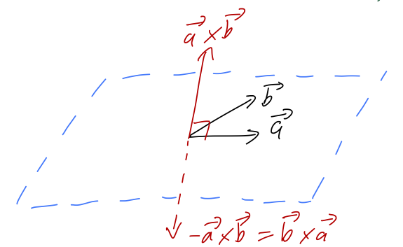
Deciding which of these two vectors to call the positive cross product is a choice of convention - which means it’s an arbitrary choice that we can make once, but then we have to keep that choice consistent. We will follow the standard physics convention, which is the right-hand rule: if you hold out your right hand with the thumb pointing in the direction of \vec{A} and your fingers in the direction of \vec{B}, then your palm points in the direction of \vec{A} \times \vec{B}. Try it with my diagram above!
The right-hand rule also fixes an ambiguity in our rectangular coordinates, which is that we could have picked either of these sets of axes:
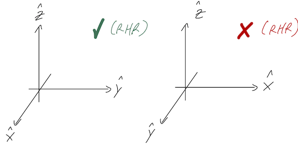
We always define our rectangular coordinates so that positive \hat{z} is a right-hand rule cross product of \hat{x} with \hat{y}. In other words, the directions of our rectangular unit vectors always satisfy: \hat{x} \times \hat{y} = \hat{z} \\ \hat{y} \times \hat{z} = \hat{x} \\ \hat{z} \times \hat{x} = \hat{y}. This is only one choice of convention, and not three; the first equation actually forces the other two to be true. An easy way to remember all three of these at once is to notice that they are all cyclic permutations: if you shift every vector to the left one spot, wrapping back around to the right at the left end, then you get the next formula.
There is a general, mechanical formula for the cross product in rectangular components, using a three-by-three matrix determinant: \vec{a} \times \vec{b} = \left|\begin{array}{ccc} \hat{x}&\hat{y}&\hat{z}\\ a_x&a_y&a_z\\ b_x&b_y&b_z\end{array}\right| \\ = (a_y b_z - a_z b_y) \hat{x} - (a_x b_z - a_z b_x) \hat{y} + (a_x b_y - a_y b_x) \hat{z}. We will use this a couple of times this semester, and you’ll see lots more of it next semester in classical mechanics 2.
Now back to angular momentum, \vec{\ell} \equiv \vec{r} \times \vec{p}. It’s very important to stress that, unlike linear momentum, this depends strongly on what the origin of our coordinate system is! Consider the following example: we have a 1 kg mass moving in a straight line at v = 2 m/s. Here’s a sketch with two possible coordinate systems:
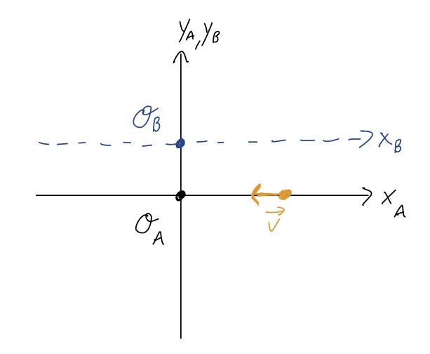
The linear momentum of the particle is the same in both coordinate systems, \vec{p} = (-2,0,0)\ {\textrm{kg}} \cdot {\textrm{m}} / {\textrm{s}}. However, the angular momentum is different: \vec{\ell}_A = \vec{r}_A \times \vec{p} = (4,0,0) \times (-2, 0, 0) = (0,0,0)\ {\textrm{kg}} \cdot {\textrm{m}}^2 / {\textrm{s}} \\ \vec{\ell}_B = \vec{r}_B \times \vec{p} = (4, -2, 0) \times (-2, 0, 0) = (0,0,-4)\ {\textrm{kg}} \cdot {\textrm{m}}^2 / {\textrm{s}}
(check the direction with the right-hand rule!) Of course, this isn’t really a fundamental difference: if I set up a third coordinate system with origin \mathcal{O}_C which is moving to the left at 2 m/s, then the linear momentum will change to \vec{p}_C = (0,0,0). Momentum is something that we define to make sense of a physical system, but all that really matters is the actual motion is the same no matter what coordinates we choose. (I stress this point here because it often catches people off-guard that angular momentum can change even if your coordinates aren’t moving.)
In the presence of forces, \vec{p} will change, and therefore \vec{L} can also be changed by forces. To see exactly how, we just take the time derivative: \frac{d\vec{\ell}}{dt} = m\frac{d}{dt} \left(\vec{r} \times \dot{\vec{r}} \right) \\ = m \dot{\vec{r}} \times \dot{\vec{r}} + m \vec{r} \times \ddot{\vec{r}} \\ = \vec{r} \times \vec{F}, where on the last line the first term vanished since it’s the cross product of a vector with itself, and in the second term we plugged in Newton’s second law. This cross product of distance and force is called the torque, \vec{\Gamma} \equiv \vec{r} \times \vec{F}. (Some references will use \tau instead of \Gamma for torque, so beware.) This gives us a rotational version of Newton’s second law, \vec{\Gamma} = \frac{d\vec{\ell}}{dt}.
We can identify a new conservation law from the last equation we wrote above: if there is no net torque on a point mass, \vec{\Gamma} = 0, then angular momentum is conserved - d\vec{\ell} / dt = 0. Note that this can be true even if there is a net force, as long as \vec{r} \times \vec{F} = 0.
Of course, this isn’t very useful for a single point mass! There are not many situations where there is a net force but no torque for the entire motion of a single particle, just because \vec{r} will generally change with time. The good news is that like conservation of linear momentum, this law also applies to collections of masses. Breaking out our trusty set of N point masses \{m_\alpha \}, it can be shown that if we define the total angular momentum \vec{L} \equiv \sum_{\alpha=1}^N \ell_\alpha, then \dot{\vec{L}} = 0 if the net external torque is zero, and more generally, \vec{\Gamma}_{\textrm{ext}} = \frac{d\vec{L}}{dt}.
(I am not going to do the proof in class - it’s another round of sums, but this time with cross products added in. Taylor shows this result in chapter 3.5, and I encourage you to have a look.)
As with conservation of linear momentum, a nice application of this conservation law is learning things about horribly complicated systems, so long as they have no external torques acting on them. The formation of the solar system, for example, was a horribly messy and complicated process spanning billions of years. However, from the simple fact that the planets currently have a net angular momentum (all of the orbits go the same way, which is the same way the Sun is spinning!), we know that whatever primordial structure the solar system formed from must have been spinning, and we can even relate its rotational speed to its size!
This is especially useful in combination with the center of mass (CM)! It turns out that for any extended object, we can decompose its motion into two parts: the motion of the CM itself, treating it like a point particle, and then rotation of the object about the CM. The latter subject is fairly complicated, but you’ll see it worked out in detail next semester, and it’s much, much easier to study rotation using the CM of an object instead of using an arbitrary set of coordinates.
There are a couple of immediate applications that we could try to work through - Taylor shows a few examples, including a version of Kepler’s second law. But these are specialized examples, especially the planetary motion one, and I think it’s better to put them off until you’re really prepared to tackle the problem of rotation and angular momentum in full.
In the next chapter, we’ll move on to consider energy and work, as well as the force of gravity.