2 Projectile motion with air resistance
2.1 Ordinary differential equations
As we’ve started to see, solving equations of motion in general requires the ability to deal with more general classes of differential equations than the simple examples from first-year physics. Before we go back to mechanics, let’s start to think about the general theory of differential equations and how to solve them.
Specifically, we’ll begin with the theory of ordinary differential equations, or “ODEs”. The opposite of ordinary is a partial differential equation, or “PDE”, which contains partial derivatives; an ordinary DE has only regular (total) derivatives, or in other words, all of the derivatives are with respect to one and only one variable. Newtonian mechanics problems are always ODEs, because we only have derivatives with respect to time in the second law.
Now, a very important fact about differential equations is that their solutions alone are not unique; we need more information to find a complete solution. As a simple example, consider the equation \frac{dy}{dx} = 2x You can probably guess right away that the function y(x) = x^2 satisfies this equation. But so does y(x) = x^2 + 1, and y(x) = x^2 - 4, and so on! In fact, this equation is simple enough that we can integrate both sides to solve it: \int dx \frac{dy}{dx} = \int dx 2x \\ y(x) = x^2 + C remembering to include the arbitrary constant of integration for these indefinite integrals. So the equation alone is not enough to give us a unique solution. But in order to fix the constant C, we just need a single extra piece of information. For example, if we add the condition y(0) = 1 then y(x) = x^2 + 1 is the only function that will work.
Now that we’re going to be writing a lot of integrals, a brief comment on integral notation to avoid some common confusion. In mathematics, the most common convention for integrals is that the differential which indicates what variable we are integrating over is at the end:
\int x^2 dx = \frac{1}{3} x^3
This lets you easily and clearly do things like mixing indefinite integrals with other functions of f: \int x^2 dx + \frac{2}{3} x^3 = x^3.
On the other hand, in physics a more common convention (and the one we will use!) is to put the differential at the start of the integral, next to the integral sign: \int dx\ x^2 = \frac{1}{3} x^3.
This will make writing the second equation above look ambiguous, but I can fix that by using parentheses/brackets: \int dx\ \left( x^2 \right) + \frac{2}{3} x^3 = x^3.
This seems obviously worse, and it is, but in physics we rarely write equations like this! Typically when we integrate over a variable, it will be a definite integral and that variable won’t appear in the resulting equation. We also do a lot more multi-dimensional integrals, where I would say the physics notation has a nice advantage - it shows clearly which integral is using which variable: compare \int_0^1 \int_0^3 \int_{-1}^{1} \sqrt{x^2 + y^2 + z^2} dx dy dz (math convention) with \int_0^1 dz \int_0^3 dy \int_{-1}^{1} dx \sqrt{x^2 + y^2 + z^2} (physics convention), I think the second one is much clearer!
What if we have a second-order derivative to deal with, like in Newton’s second law \vec{F} = m \ddot{\vec{r}}? To solve this equation (or indeed any ODE that has a second-order derivative), we will need two conditions to find a unique solution. One way to think of this is to think about solving the equation by integration; to reverse both derivatives on d^2 \vec{r} / dt^2, we have to integrate twice, getting two constants of integration to deal with.
This statement turns out to be true in general, even though we can’t solve most ODEs just by integrating directly: every derivative that has to be reversed gives us one new unknown constant of integration. Notice that I’ve been using a calculus vocabulary term, which is ‘order’: the object \frac{d^{(n)} f}{dx^n} = \left( \frac{d}{dx} \right)^n f(x) is called the n-th order derivative of f with respect to x. The same vocabulary term applies to ODEs: the order of an ODE is equal to the highest derivative order that appears in it. (So Newton’s second law is a second-order ODE; to solve it we need two conditions, usually the initial position and initial velocity.)
Here’s another way to understand how order relates to the number of conditions. Using Newton’s law as an example again, notice that in full generality, we can rewrite it in the form \frac{d^2 \vec{r}}{dt^2} = f\left(\vec{r}, \frac{d \vec{r}}{dt} \right).
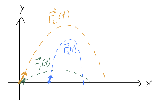
In other words, if at any time t we know both the position and the velocity, then we can just plug in to this equation to find the acceleration at that time. But then because acceleration is the time derivative of velocity, we can predict what will happen next! Suppose we start at t=0. Then a very short time later at t = \epsilon, \frac{d\vec{r}}{dt}(\epsilon) = \frac{d\vec{r}}{dt}(0) + \epsilon \frac{d^2 \vec{r}}{dt^2}(0) + ... \\ \vec{r}(\epsilon) = \vec{r}(0) + \epsilon \frac{d\vec{r}}{dt}(0) + ... Now we know the ‘next’ values of position and velocity for our system. And since we know those, we plug in to the equation above and get the ‘next’ acceleration, d^2 \vec{r} / dt^2(\epsilon). Then we repeat the process to move to t = 2\epsilon, and then 3\epsilon, and so on until we’ve evolved as far as we want to in time. Depending on what choices we made for the initial values, we’ll build up different curves for \vec{r}(t):
This might sound like a tedious procedure, and it is, but this process (or more sophisticated versions of it) are exactly how numerical solution of differential equations are found. If you use the “NDSolve” function in Mathematica, for instance, it’s doing some version of this iterative procedure to give you the answer. But more importantly, I think this is a more physical way to think about what initial conditions mean, and why we need n of them for an n-th order ODE.
As a side benefit, this construction also establishes uniqueness of solutions: once we fully choose the initial conditions, there is only one possible answer for the solution to the ODE. For Newtonian physics, this means that knowing the initial position and velocity is enough to tell you the unique possible physical path \vec{r}(t) that the system will follow.
Keep in mind that the construction above makes use of initial values, where we specify all of the conditions on our ODE at the same point (same value of t here.) This is a special case of the more general idea of boundary conditions, which can be specified in different ways. (For example, we could find a unique solution for projectile motion by specifying y(0) = y(t_f) = 0 and solving from there to see when our projectile hits the ground again.)
2.1.1 Classifying ODEs and general solutions
Numerical solution is a great tool, but whenever possible we would prefer to be able to solve equations by hand - this is more powerful because we can solve for a bunch of initial conditions at once, and we can have a better understanding of what the solution means.
This brings us to classification of differential equations. There is no algorithm for solving an arbitrary differential equation, even an ODE, and many such equations have no known solutions at all (at which point we go back to numerics.) But there is a long list of special cases in which a solution is known, or a certain simplifying trick will let us find one. Because analytic solution of ODEs is all about knowing the special cases, it’s very important to recognize whether a given equation we find in the wild belongs to one of the classes we have some trick for.
The first such classification we’ll go learn to recognize is the linear ODE (the opposite of which is nonlinear.) To explain this clearly, remember that a linear function is one of the form y(x) = mx + b. To state this in words, the function only modifies x by addition and multiplication with some constants, m and b. A linear differential equation, then, is one in which the unknown function and its derivatives are only multiplied by constants and added together.
For example, if we’re solving for y(x), the most general linear differential equation looks like a_0(x) y + a_1(x) \frac{dy}{dx} + a_2(x) \frac{d^2y}{dx^2} + ... + b(x) = 0. This is a little more complicated since we have two variables now, but if you think of freezing the value of x, then all of the a’s and b are constant and it’s clearly a linear function.
Linearity turns out to be a very useful condition. This isn’t a math class so I won’t go over the proof, but there is a very important result for linear ODEs:
A linear ODE of order n has a unique general solution which depends on n independent unknown constants.
The term “general solution” means that there is a function we can write down which solves the ODE, no matter what the initial conditions are. This function has to contain n constants that can be adjusted to match initial conditions (as we discussed above), but otherwise it is the same function everywhere.
To avoid a common misconception, it’s just as important to be aware of the opposite of the above statement: if we have non-linear ODE, in many cases there is no general solution. There is still always a unique solution if we fully specify the initial values. But for a non-linear ODE the functional form of the solution can be different depending on what the initial values are! See Boas 8.2 for an example.
Alright, so it’s great that we know a general solution is out there, but how do we find it in practice? The answer depends a bit on what kind of equation we have.
The following example is a bonus because you have likely seen this equation before! But if you haven’t, or if you’re not too comfortable with the idea of a “general solution” yet, then you should go through this.
Let’s solve the following ODE: \frac{d^2y}{dx^2} = +k^2 y There is a general procedure for solving second-order linear ODEs like this, but I’ll defer that until later. To show off the power of general solutions, I’m going to use a much cruder approach: guessing. (If you want to sound more intellectual when you’re guessing, the term used by physicists for an educated guess is “ansatz”.)
Notice that the equation tells us that when we take the derivative of y(x) twice, we end up with a constant times y(x) again. This should immediately make you think about exponential functions, since d(e^x)/dx = e^x. To get the constant k out from the derivatives, it should appear inside the exponential. So we can guess y_1(x) = e^{+kx} and easily verify that this indeed satisfies the differential equation. However, we don’t have any arbitrary constants yet, so we can’t properly match on to initial conditions. We can notice next that because y(x) appears on both sides of the ODE, we can multiply our guess by a constant and it will still work. So our refined guess is y_1(x) = Ae^{+kx}. This is progress, but we have only one unknown constant and we need two. Going back to the equation, we can notice that because the derivative occurs twice, a negative value of k would also satisfy the equation. So we can come up with a second guess: y_2(x) = Be^{-kx}. This is very similar to our first guess above, but it is in fact an independent solution, independent meaning that we can’t just change the values of our arbitrary constants to get this form from the other solution. (We’re not allowed to change k, because it’s not arbitrary, it’s in the ODE that we’re solving!)
Finally, we notice that the combination y_1(x) + y_2(x) of these two solutions is also a solution if we plug it back in. So we have y(x) = Ae^{+kx} + Be^{-kx} This is a general solution: it’s a solution and it has two distinct unknown constants, A and B. Thanks to the math result above, if we have a general solution to a linear ODE, we know that it is the general solution thanks to uniqueness.
The whole procedure we just followed might seem sort of arbitrary, and indeed it was, since it was based on guessing! For different classes of ODEs, there will be a variety of different solution methods that we can use. The power of the general solution for linear ODEs is that no matter how we get there, once we find a solution with the required number of arbitrary constants, we know that we’re done. Often it’s easiest to find individual functions that solve the equation, and then put them together as we did here. (Remember, solving ODEs is all about recognizing special cases and equations you’ve seen before!)
Now let’s start to look at some specific methods for solving differential equations. We’re going to begin with first-order ODEs only, because that will open up a new class of physics problems for us to solve: projectile motion with air resistance. Later in the semester, we’ll come back to second-order ODEs.
2.1.2 Separable first-order ODEs
A unique feature of first-order ODEs is that we can sometimes solve them just by doing integrals. A first-order ODE is separable if we can write it in the form F(y) dy = G(x) dx where F(y) and G(x) are just any arbitrary function. Once we’ve reached this form, we can just integrate both sides and end up with an equation relating y to x, which is our solution. This method works even if the ODE is not linear.
A quick aside: splitting the differentials dy and dx apart like this is something physicists tend to do much more than mathematicians (although Boas does it!) Remember that dx and dy do have meaning on their own, as they’re defined to be infinitesmal intervals when we define the derivative dy/dx. That being said, if you’re unsettled by the split derivative above, you can instead think of a separable ODE as one written in the form F(y) \frac{dy}{dx} = G(x) Then we can integrate both sides over dx, \int F(y) \frac{dy}{dx} dx = \int G(x) dx The integral on the left becomes \int F(y) dy by a u-substitution. After we do the integrals, we just have a regular equation to solve for y. The simplest case is when F(y) = 1, i.e. if we have \frac{dy}{dx} = G(x) \\ \int dy = \int G(x) dx \\ y = \int G(x) dx + C (notice that we get one overall constant of integration from the indefinite integrals, just as needed to match the single initial condition for a first-order ODE.)
Solve the following ODE: x \frac{dy}{dx} - y = xy
Solution:
This might not be obviously separable, but let’s do some algebra to find out. We’ll put the y’s together first: x \frac{dy}{dx} = y(1+x) Then divide by x and by y: \frac{1}{y} \frac{dy}{dx} = \frac{1+x}{x} Nice and separated! Next, we split the derivative apart and integrate on both sides: \int \frac{dy}{y} = \int dx\ \frac{1+x}{x} The left-hand side integral will give us the log of y. On the right, it’s easiest to just divide out and write it as 1/x + 1, which gives us two simple integrals: \ln y + C' = \int dx\ \left(1 + \frac{1}{x} \right) = x + \ln x + C'' Just to be explicit, I kept both unknown constants here since we did two indefinite integrals. But since C' and C'' are both arbitrary, and we’re adding them together, we can just combine them into a single constant C = C'' - C'.
Now we need to solve for y. Start by exponentiating both sides: y(x) = \exp \left( x + \ln x + C'' \right) \\ = e^x e^{\ln x} e^{C''} \\ = B x e^x defining one more arbitrary constant. (Since we haven’t determined what the constant is yet by applying boundary conditions, it’s not so important to keep track of how we’re redefining it.)
Finally, we can impose a boundary condition to find a particular solution. Let’s say that y(2) = 2. We plug in to get an equation for B: y(2) = 2 = 2B e^2 \\ \Rightarrow B = \frac{1}{e^2} = e^{-2} and so y(x) = xe^{x-2}.
2.1.3 Linear first-order ODEs
(Note: this solution is discussed in Boas 8.3, but I’m borrowing a little bit of terminology from later sections of chapter 8 to put it in context.)
It turns out that there is a nice and general way to find solutions linear first-order ODEs. The combination of linear and first-order is very restrictive: any such ODE must take the form \frac{dy}{dx} + P(x) y = Q(x).
This is a good place to introduce another technical term, which is homogeneous. A homogeneous ODE is one in which every single term depends on the unknown function y or its derivatives. The equation above does not satisfy this condition, because the Q(x) term on the right doesn’t have any y-dependence; thus, we say this equation is inhomogeneous (some books will use “nonhomogeneous” instead.)
Now, there is another equation which closely related to the one above: \frac{dy_c}{dx} + P(x) y_c = 0. The “c” here stands for complementary; this equation is called the complementary equation to the original. Setting Q(x) to zero gives us an equation that is homogeneous.
Better yet, this equation is separable too: we can readily find that \frac{dy_c}{y_c} = -P(x) dx or doing the integrals, y_c(x) = A e^{-\int dx P(x)}. Of course, this is only a solution if Q(x) happens to be zero. But it turns out to be part of the solution for any Q(x). Suppose that we are able to find some other function y_p(x), which is a particular solution that satisfies the original, inhomogenous equation. Then y(x) = y_c(x) + y_p(x) is also a solution of the full equation. This is easy to see by plugging in: \frac{dy}{dx} + P(x) y = \frac{d}{dx} \left( y_c(x) + y_p(x) \right) + P(x) (y_c(x) + y_p(x)) \\ = \left[\frac{dy_c}{dx} + P(x) y_c(x) \right] + \left[ \frac{dy_p}{dx} + P(x) y_p(x) \right] \\ = 0 + Q(x). This might not seem very useful, because we still have to find y_p(x) somehow. But notice that y_c(x) always has the arbitrary constant A in it. That means that y(x) = y_c(x) + y_p(x) is the general solution to our original ODE (the unique one, because it’s linear, remember!)
This isn’t a mechanics example, but it happens to be one of the simpler cases of a first-order and inhomogeneous ODE problem, so let’s do it anyway. We have an electric circuit consisting of a battery supplying voltage V_0, a resistor with resistance R, and a capacitor with capacitance C:
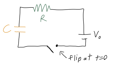
If the capacitor begins with no charge at t=0, we want to describe the current I(t) flowing in the circuit as a function of time. Now, current is the flow of charge, so the charge Q on the capacitor will satisfy the equation I = \frac{dQ}{dt}. The other relevant circuit equations we need are V = IR for the resistor, and Q = CV for the capacitor. Putting these together, we find that the equation describing the circuit is R \frac{dQ}{dt} + \frac{Q}{C} = V_0. The complementary equation is R\frac{dQ_c}{dt} + \frac{Q_c}{C} = 0 which is nice and separable: \frac{dQ_c}{Q_c} = -\frac{1}{RC} dt Integrating gives \ln Q_c = -\frac{t}{RC} + K \Rightarrow Q_c(t) = K' e^{-t/(RC)} Now we need to find the particular solution Q_p. Fortunately, because the right-hand side is just a constant, it’s easy to see that a constant value for Q_p will give us what we want. Specifically, if Q_p = CV_0 then the equation is satisfied, since the derivative term just vanishes.
Finally, we put things together and apply our boundary condition, Q(0) = 0: Q_c(0) + Q_p(0) = 0 = K' e^{-0/(RC)} + CV_0 = K' + CV_0 finding that K' = -CV_0, and thus the finished result is Q(t) = CV_0 \left(1 - e^{-t/(RC)} \right).
So far, everything I’ve said is actually fairly general: this same approach with complementary and particular solutions will be something we use a lot when we get to second-order ODEs.
For any first-order linear ODE, there is actually a trick which will always give you the particular solution for any functions P(x) and Q(x). However, it’s a little complicated to write down, and we won’t need it often. So I won’t cover that here, and instead I’ll refer you to Boas 8.3 for the result. This is one of those formulas that you should know exists, but it’s not worth memorizing - if you find you need it, you can go look it up.
Here, you should complete Tutorial 2A on “Ordinary differential equations”. (Tutorials are not included with these lecture notes; if you’re in the class, you will find them on Canvas.)
2.2 Projectile motion and air resistance
Let’s come back to physics and put our theory of first-order ODEs to use. Air resistance problems turn out to be the perfect application, because air resistance gives a force which depends on the velocity of the object moving through the air. Of course, Newton’s second law is generally a second-order ODE, \vec{F} = m\ddot{\vec{r}}. But in the special case that the force only depends on the velocity \vec{v} = d\vec{r}/dt, we can rewrite this as \vec{F}(\vec{v}) = m\dot{\vec{v}} which we can treat as a first-order ODE.
Before we get to the math, let’s talk about the physics of air resistance, also known as drag for short (not to be confused with the regular friction that you get if you drag an object across a rough surface.) As the name implies, this is a force which resists motion, which explains why it depends on speed.
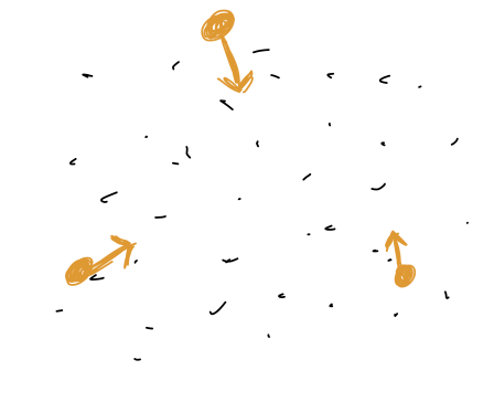
What do we know about the nature of the drag force \vec{f}(\vec{v})? First of all, the air is (to a very good approximation) isotropic, i.e. it is uniform enough that it looks the same no matter which direction we move through it.
This means that the magnitude of the drag force should only depend on the speed, i.e. \vec{f}(\vec{v}) = \vec{f}(v). If the object moving through the air is also very symmetrical (like a sphere), then the orientation of our object also doesn’t matter, and we expect the direction of the force to be opposite the direction of motion, \vec{f}(v) = -f(v) \hat{v}. There are many examples of systems for which this second equation does not hold. Taylor gives the example of an airplane, which experiences a lift force clearly not in the same direction of its motion. A more mundane example is a frisbee, for which air resistance actually provides a stabilizing force that keeps it from tumbling while in the air. But there are lots of interesting systems where this relation does hold, so we’ll assume it for the rest of this section.
Unfortunately, this is still way too general: we need some information about what the function f(v) is before we can hope to make any progress. There are two effects that are important in the interactions between a fluid and an object traveling through it, and they will give us linear and quadratic dependence on the speed respectively. So the most general drag force we will study is f(v) = bv + cv^2. Now, Taylor points out that this is valid at “lower speeds”, and that there are other effects that are important near the speed of sound. In fact, another way to derive this form for f(v) is through Taylor series expansion. But we should be careful, because this is a physics class, and series expanding in v doesn’t really make sense - it has units! If we really want to expand, we need to expand in something dimensionless; equivalently, we need to answer the question “v is small compared to what?”
The answer is what I already said: v should be small compared to v_s, the speed of sound of air (or whatever fluid medium we are studying.) v_s is the speed at which the motion of the air molecules relative to each other will start to matter and things will get more complicated. Thus, we can write f(v) = b_0\frac{v}{v_s} + c_0 \frac{v^2}{v_s^2} + d_0 \frac{v^3}{v_s^3} + ... (there is no constant term a_0, for the simple reason that we know there is no drag force if v=0.) The beauty of this approach is that so long as we are working at speeds v \ll v_s, we can study air resistance even if we have no idea what the original function f(v) is: all we have to do is run a few experiments to measure the constants b_0, c_0, d_0 (and so on, if we care about even smaller corrections.)
This is an example of the concept of an effective theory, which has a limited range of applicability: the series expansion version of f(v) is not valid at any speed, but at small speeds it can be used to make useful predictions once we’ve done a couple experiments to set it up. This should remind you of the classical limit v \ll c from special relativity, too. I’ll come back to the idea of effective theories again later on; it’s a more common concept in physics than you may realize!
Although the generic series-expansion approach would work just fine, we will instead borrow some more advanced ideas from fluid mechanics. There are two specific effects that will give rise to the linear and quadratic terms, and will thus allow us to predict what the coefficients b and c are.
2.2.1 Microscopic origin of drag forces
Let’s begin with the linear drag force. From fluid mechanics, a constant known as the viscosity, \eta, determines how resistant the air (or whatever fluid we are moving through) is to being deformed; larger \eta means that the force exerted by adjacent layers of fluid on each other is larger. Without going into too much detail, \eta has units of N \cdot s / m^2 (see Taylor problem 2.2.)
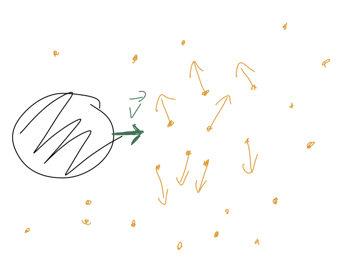
This is a low-speed effect which treats the air like a smooth, continuous medium. To see the dependence on the other properties of our moving object, consider this sketch:
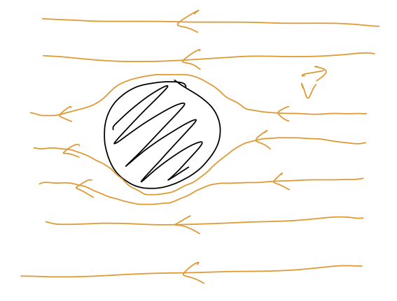
From the frame of reference of the moving object, the air is flowing across it at speed v. Near the object itself, the moving air has its path deformed around the object; the size of the deformation is proportional to the linear size of the object, D. (The sketch above only shows two dimensions: the lines of airflow are actually planes, which is why the dependence is just D.) The complete formula for a spherical object is f_{\textrm{lin}}(v) = 3\pi \eta D v. where D is specifically the diameter of the sphere. For air at STP and a spherical object, Taylor goes on to give the result b = \beta D,\ \ \beta = 1.6 \times 10^{-4}\ N \cdot s / m^2 which is convenient for talking about air resistance in particular.
Next, we have the quadratic drag force. This is a more violent effect, arising at higher speeds. Basically, if the speed of our object is large enough, the air doesn’t have enough time to flow smoothly out of the way, and instead the individual air molecules are swept up and kicked out of the path of our object:
(This is an example of turbulent flow, as opposed to the smooth laminar flow in the linear regime.) We can think of there being two different v-dependent effects here. First, the speed at which the air molecules have to get out of the way will increase proportional to v. Second, for larger v our object will simply run into more air molecules per unit time. So indeed, we expect a quadratic dependence v^2 for this force.
Two other factors influence how many air molecules are swept up per unit time. First, the cross-sectional area A of our object - the depth of the object doesn’t matter because they’re just scattering out of its path completely. Second, the density of the air, \rho. (If we’re counting molecules it’s the number density \rho/m_{\textrm{air}} that matters, but we’re interested in the drag force, which puts the factor of m_{\textrm{air}} back in.) Thus, the final result is f_{\textrm{quad}}(v) = \frac{1}{2} C_D \rho A v^2 This introduces one more physical quantity, the dimensionless number C_D which is known as the drag coefficient. This number is usually between 0 and 1, and determines how streamlined the object is (for a smoother object, the air doesn’t have to be deflected completely out of the way as soon as the front of the object hits it.) For a sphere, C_D \approx 0.5; a reasonably aerodynamic car has C_D \approx 0.25, and a 747 jumbo jet has C_D \approx 0.03.
Once again, we can specialize to air at STP and a spherical object, and Taylor gives the result c = \gamma D^2,\ \ \gamma = 0.25\ N \cdot s^2 / m^4. This is handy, but do keep in mind that it assumes a sphere; if you want to study air resistance for an object that you know the drag coefficient for, you should adjust the formula, multiplying by C_D / (1/2) = 2C_D. (The extra 2 deals with the fact that C_D = 1/2 for a sphere.)
Unfortunately, the general drag force f(v) = bv + cv^2 is still slightly too complicated to work with analytically for solving the motion. We will talk about that general case, but first we’ll try to understand two restricted cases. In the linear drag regime, the bv term is relatively large and we can ignore the quadratic term completely; this is obviously where v is very small. In the other limit where v is very large, we can ignore the linear term and solve in the quadratic drag regime.
Of course, we can’t just say “v is really big”, we have to be quantitative - the size of b and c matters too! We should really just compare the forces directly: \frac{f_{\textrm{quad}}}{f_{\textrm{lin}}} = \frac{cv^2}{bv} = \frac{C_D \rho Av^2}{2 \eta D v} = \left( \frac{C_D A}{6\pi D^2} \right) \frac{D \rho v}{\eta} The combination C_D A / (6\pi D^2) is some dimensionless number which is generally not very far from 1, while the other fraction is another dimensionless combination known as the Reynolds number, R \equiv \frac{D \rho v}{\eta}. So if R \ll 1, the linear force is definitely dominant and we can ignore the quadratic term. If R \gg 1, the opposite is true and we just study the quadratic term. If R is sort of close to 1, then we probably can’t ignore either effect and need to be careful.
It’s helpful to know the ratio of these forces for air and some example objects. In his example 2.1, Taylor estimates that f_{\textrm{quad}} / f_{\textrm{lin}} \sim 600 for a baseball moving at 5 m/s, \sim 1 for a raindrop at 0.5 m/s, and \sim 10^{-7} at 5 \times 10^{-5} m/s in the Millikan oil drop experiment. From the way the Reynolds number depends on D and v, this means that air resistance for everyday objects is almost always dominantly quadratic.
To summarize, the general drag force takes the form f(v) = bv + cv^2, where for air at STP and an object with diameter D we have b = \beta D, c = \gamma D^2, with \beta = 1.6 \times 10^{-4}\ N \cdot s / m^2,\\ \gamma = 0.25\ N \cdot s^2 / m^4. However, we know that the real formulas for the drag coefficients are b = 3\pi \eta D \Rightarrow \beta = 3\pi \eta, \\ c = \frac{1}{2} C_D \rho A \Rightarrow \gamma = \frac{1}{2} C_D \rho (A/D^2). where \eta and \rho are the viscosity and density of the medium. We will rarely use these formulas in full, but in many situations it is useful to know how they would scale if we have another situation which we can compare to air at STP. For example, water is about 50 times more viscous than air. So if we are interested in linear drag acting on an object in water, we can just multiply the value of \beta in air by 50.
Since I mentioned water, there is one more microscopic force that is present for objects moving in a fluid medium: the buoyant force. The buoyant force occurs when we move in a fluid that itself exists within a constant gravitational field g. Roughly speaking, an object immersed in fluid feels the combined weight of all of the fluid molecules above a given point, which results in increased pressure proportional to the depth. The difference in pressure between the bottom and top of a solid object gives rise to a buoyant force pushing against gravity, F_b = -\rho V \vec{g}, where \rho is the fluid density and V is the solid volume of the immersed object. This can be stated in words as “Archimedes’ principle”: the magnitude of the buoyant force is equal to g times the mass of the fluid displaced (pushed out of the way) by our solid object.
Taylor doesn’t really talk about buoyant force, and for most applications involving air resistance, we can safely ignore it, as long as the density of the objects moving around is much larger than the density of air (so that mg will be much greater than \rho V g.) However, in physics it’s always important to know when it’s safe to ignore something. Obviously if we wanted to study, say, the motion of a hot-air balloon with air resistance - or drag forces of relatively light objects underwater - then we’d want to include buoyant force as well.
Which has the larger quadratic drag coefficient c: a human being moving through air at STP, or a baseball moving through water (which is about 800 times more dense than air?)
Answer:
The formula for the quadratic drag coefficient is c = \frac{1}{2} C_D \rho A.
In this example we’re changing all three quantities, although we might suspect that C_D isn’t incredibly different for a human (estimates I can find give roughly C_D \sim 1 for a human who isn’t trying to curl into a ball, so about double the coefficient of a sphere.) So this is mainly about comparing the changes in density and in cross-sectional area - and we were given the change in density.
Sitting here at my desk, I can easily look up accurate values for the size of a baseball and a human; but first I’ll try to deal with the problem the way you would in class, which is using estimation (a very useful physics skill!) I know that the average human is on the order of 2 meters tall and maybe half a meter wide, so let’s say that A_{\textrm{ human}} = 1\ {\textrm{m}}^2.
On the other hand, a baseball is pretty small, but not tiny; if I imagine stacking baseballs together near a meter stick, I would say I can probably fit at least 10 of them, so I’ll say that a baseball has a diameter of about 10 cm. So the cross-sectional area is A_{\textrm{baseball}} \sim 4\pi (0.05\ {\textrm{m}})^2 \approx 2.5 \times 10^{-2}\ {\textrm{m}}^2.
Some mental math: 4\pi is about 10, and I can decompose (0.05)^2 = (5 \times 10^{-2})^2 = 25 \times 10^{-4} which gives me the result above. I’ve rounded lots of things off very badly, so I don’t really trust my accuracy to be much better than order of magnitude (i.e. a factor of 10), but since my initial estimates were probably order of magnitude accuracy at best, that’s fine with me!
Now I can compute the ratio of drag coefficients: if I ignore the C_D, I find that
\frac{c_{\textrm{ baseball}}}{c_{\textrm{human}}} \approx \frac{\rho_{\textrm{water}} A_{\textrm{baseball}}}{\rho_{\textrm{air}} A_{\textrm{human}}} = 800 \frac{0.025}{1} \approx 20. Although I did lots of pretty rough approximations, I think I can safely conclude that the baseball in water has a larger c.
Now I can use the internet to find more accurate results: the diameter of a regulation MLB baseball is about 7.4 cm, so my estimate was actually pretty close! The cross-sectional area of a skydiver is closer to about 0.5 {\textrm{m}}^2, since 1 meter wide is definitely a bad overestimate. If I include the fact that the drag coefficient C_D is about double for a human, I find the improved estimate \frac{c_{\textrm{baseball}}}{c_{\textrm{human}}} \approx 110. Using more accurate numbers really improves our estimate - but it doesn’t change the qualitative answer, which is that c is larger for the baseball in this situation.2.2.2 Freefall and terminal velocity
Before we move on to actually solving any of the ODEs that appear with drag forces, it’s a worthwhile exercise to first study how to set up the equations of motion for the simple and useful case of free-falling motion. We will solve the free-fall equations of motion eventually, both for linear and quadratic drag, but there’s actually some interesting math we can do before we solve them. There’s also some tricky details in setting up the equations when our forces depend on the velocity!
Here, you should complete Tutorial 2B on “Velocity-dependent forces”. (Tutorials are not included with these lecture notes; if you’re in the class, you will find them on Canvas.)
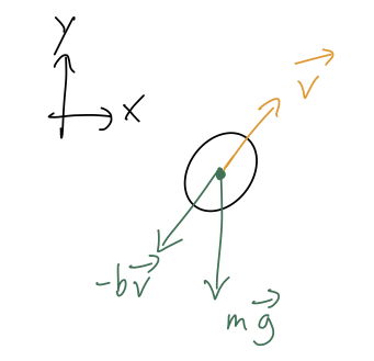
For free-fall, we can restrict ourself to a single coordinate y. The only forces are gravity and the drag force - both linear and quadratic, but they will always point in the same direction (opposite \vec{v}), so we can draw them together as a single vector \vec{f}_v for now. Here is the free-body diagram:
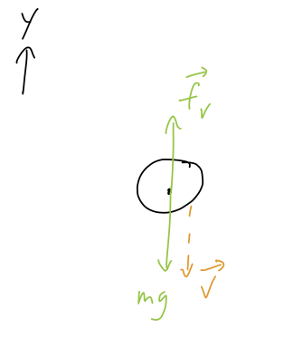
Note that this diagram assumes that velocity is pointing down in this instant - as you explored on the tutorial, this will change if the ball is moving up instead! (If you’re comparing to Taylor, note that he assumes y is pointing down and there are some minus-sign differences as a result.)
What you should have found from the tutorial is the following equation of motion for a downwards-moving ball, with the quadratic drag coefficient c set to zero: \dot{v}_y = -g - \frac{b}{m} v_y. (Don’t forget, v_y is positive for upwards motion, negative for downwards!)
We can already notice something interesting just from this equation of motion, without actually solving it yet. There is a particular speed for which the right-hand side of the equation will vanish: v_{y} = -v_{\textrm{ter}} = -\frac{mg}{b}.
For an object free-falling at this speed, the drag force balances gravity and there is no acceleration (\dot{v}_y = 0). This speed is known as the terminal velocity, because it is the maximum possible speed that can be reached for an object dropped from rest. (Note that I took out a minus sign, so that the terminal “velocity” will always be a positive number, matching Taylor’s definition.)
In fact, this is the final speed that will be reached for any initial speed, even if we launch an object faster than v_{\textrm{ter}}! You can convince yourself (following the tutorial) that for v_y < -v_{\textrm{ter}}, we will find \dot{v}_y > 0 so that the object will decelerate until it reaches v_{\textrm{ter}} and the forces balance.
What about the opposite case, where we have only quadratic drag? Setting b = 0 in the equations of motion from the tutorial instead, you should have (for downwards motion v_y < 0) \dot{v}_y = -g + \frac{c}{m} v_y^2. Note that matching the diagram, gravity and drag point in opposite directions. Here we see again that there is another terminal velocity at which the forces balance and the acceleration is zero: v_{\textrm{ter, c}} = \sqrt{\frac{mg}{c}}.
What does the equation of motion for v_y > 0 and quadratic drag only look like? Is the terminal velocity the same as what we just found, or does something else happen in this case?
Answer:
If v_y > 0, then the equation of motion becomes \dot{v}_y = -g - \frac{c}{m} v_y^2\ \ (v_y > 0). In this case, there is no terminal velocity. Physically, this makes sense because if our object is moving upwards, gravity and drag are both pointing down, and the forces can’t balance. Eventually our object will turn around and start to fall, and we’ll end up in the v_y < 0 case and approach the terminal velocity v_{{\textrm{ter}},c}. However, we can’t use our quadratic solution to describe this motion, because the object has to come to a stop before it turns around, and the linear air resistance will start to matter!
Now let’s finally put our ODE skills to work! Following the book, we will start by solving the case of linear drag, which is less practically interesting but easier to work with mathematically.
2.3 Linear drag
The first example I will consider here is the simplest, which is horizontal motion with linear drag. (You can realize this experimentally by immersing a frictionless cart on a surface in some viscous liquid, like honey or molasses.) If we just start the cart off with some initial speed v_0 and release it, the only force acting will be drag:
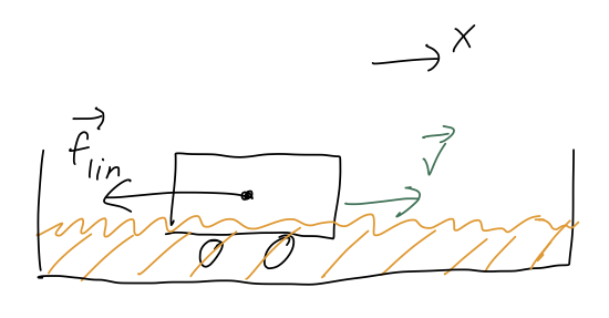
Newton’s second law is thus m \ddot{x} = -b \dot{x}. As I said a little while back, we can turn this into a first-order ODE by taking v_x = \dot{x} as our unknown variable, leading to the equation \dot{v}_x = -\frac{b}{m} v_x.
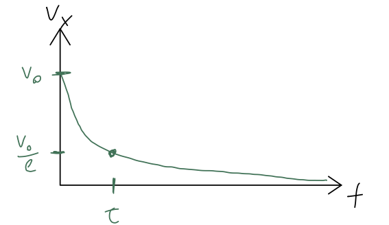
Now let’s find the solution. This is a separable ODE, so we can solve it right away. Separating v_x and t out gives \frac{dv_x}{v_x} = -\frac{b}{m} dt and then integrating leads to \ln v_x = -\frac{bt}{m} + C \Rightarrow v_x(t) = C' e^{-bt/m} and finally, using v_x(0) = v_0, the full solution is v_x(t) = v_0 e^{-t/\tau}, introducing the quantity \tau \equiv m/b, sometimes called the “natural time” or “decay time”. So, the speed as a function of time will decay to zero exponentially like so:
Although we ignored the actual position x to get here, now that we have the solution, it’s easy to reconstruct: x(t) = x(0) + \int_0^{t} dt' v_x(t') = x_0 + v_0 \int_0^t dt' e^{-t'/\tau} \\ = x_0 -\tau v_0 \left. e^{-t'/\tau} \right|_0^{t} \\ = x_0 + \tau v_0 (1 - e^{-t/\tau}). As t goes to infinity, the distance traveled by the cart approaches \Delta x_\infty = \tau v_0:
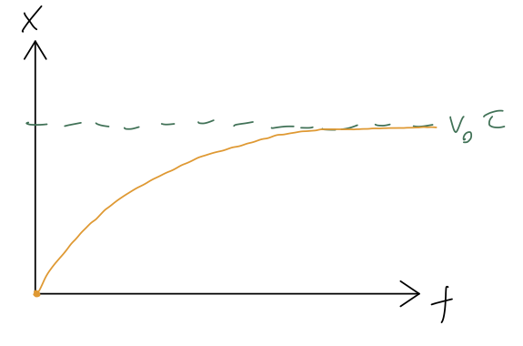
Notice that the natural time \tau popped up again: the total distance traveled by the cart when it stops is exactly the same as the distance it would have traveled with no drag in time \tau. This isn’t a deep statement: it’s more of an example of dimensional analysis, which is the idea that we can often guess the right answer (or close to it) just by putting together known quantities in the only way that their units will allow. In this case, given v_0 and \tau, the only thing we can build with units of distance is v_0 \tau.
2.3.1 Linear drag and freefall
Now that we’re warmed up, let’s move on to the more interesting case of an object in freefall. Here is the free-body diagram again:
(again, note Taylor has some minus-sign differences!) giving the equation of motion \dot{v}_y = -g - \frac{b}{m} v_y. As a reminder from above, the acceleration vanishes at the terminal velocity v_{y} = -v_{\textrm{ter}} = -\frac{mg}{b}.
Now let’s find a solution. There is more than one way to do this: Taylor shows you one way involving a u-substitution. I’ll use the method of particular solutions instead. First, we should notice that this equation is inhomogeneous, because of the g. The complementary equation is \dot{v}_{y,c} + \frac{b}{m} v_{y,c} = 0. We just solved this for horizontal motion; we know the answer is v_{y,c}(t) = Ce^{-bt/m}. Next, we need a particular solution. As before, because the inhomogeneous piece is just a constant, a constant particular solution will work: if we write v_{y,p}(t) = -\frac{mg}{b} = -v_{\textrm{ter}}, then \dot{v}_{y,p} = 0 and the full equation is satisfied. Our general solution just requires putting them together: v_y(t) = v_{y,c}(t) + v_{y,p}(t) = -v_{\textrm{ter}} + Ce^{-bt/m}. Finally, we apply our initial condition to fix the constant C: v_y(0) = v_0 = -v_{\textrm{ter}} + C \\ \Rightarrow C = v_0 + v_{\textrm{ter}} or plugging back in, and putting in the natural time \tau = m/b like we did before, v_y(t) = v_0 e^{-t/\tau} - v_{\textrm{ter}} (1 - e^{-t/\tau}).
If v_0 = 0, this looks exactly like what the x-dependence looked like for the horizontal case: the speed starts at zero and grows like an inverse exponential, asymptoting towards the (negative) terminal velocity. More generally, the dependence on the initial speed v_0 will decay exponentially, so that as we discussed any solution will approach the terminal velocity at large enough times.
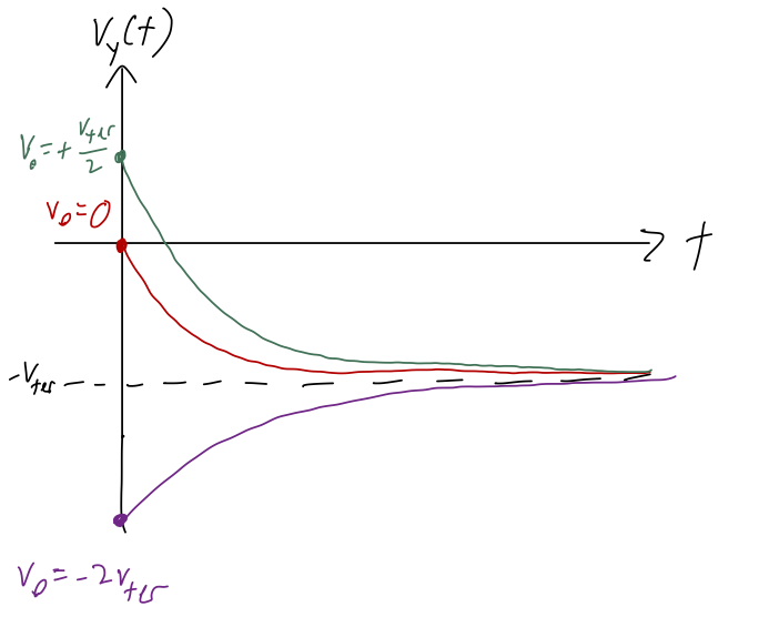
As an example, let me make a sketch of v_y(t) for a few different choices of initial conditions: v_y(0) = 0, v_y(0) = +v_{\textrm{ter}}/2, and v_y(0) = -2v_{\textrm{ter}}.
A few general tips on sketching, here: always fill in important/known points and asymptotes first. Here we expect that all of our solutions asymptote at -v_{\textrm{ter}}, so that should be the first line you draw! Then I would fill in the y-intercepts, which are the initial conditions given to us.
From that point forward, you can finish the sketch, because you know it will be a smooth and exponentially decaying curve since all the time dependence is of the form e^{-t/\tau}. (I wasn’t careful about labelling t = \tau on my sketch below, but that would be a good addition, and would help you set the scale of your exponential curve!)
If you’re having trouble visualizing the different pieces contributing here, try making a sketch or plot in Mathematica of the two terms separately, and then imagine the total curve as the sum of the two.
Here’s a sketch with the two requested initial conditions, and another one beyond v_{\textrm{ter}} just to show what happens in that case:
Finally, we can integrate once to get the position vs. time: y(t) = y(0) + \int_0^t dt' v_y(t') \\ = y_0 + v_0 \int_0^t dt' e^{-t'/\tau} - v_{\textrm{ter}} \int_0^t dt' (1 - e^{-t'/\tau}) \\ = y_0 - \tau v_0 \left. e^{-t'/\tau} \right|_0^t - v_{\textrm{ter}} t - \tau v_{\textrm{ter}} \left. e^{-t'/\tau}\right|_0^t \\ = y_0 - v_{\textrm{ter}} t + (v_0 + v_{\textrm{ter}}) \tau (1 - e^{-t/\tau}).
(Now we’re back to agreeing exactly with Taylor (2.36), because he sneaks in a sign flip on v_{\textrm{ter}} just above that equation.) Remember that v_{\textrm{ter}} by definition is always positive, but we could have a negative v_0 if the initial velocity is pointing downwards.
2.3.2 Projectile motion with linear air resistance
Remember that one of the nice things about Newton’s laws and Cartesian coordinates was that they just split apart into independent equations. In particular, suppose we want to study the problem of projectile motion in the x-y plane. The free-body diagram is:
leading to the two equations of motion
\ddot{x} = -\frac{b}{m} \dot{x}, \\ \ddot{y} = -g - \frac{b}{m} \dot{y}.
Those are exactly the two equations we just finished solving for purely horizontal and purely vertical motion! So we can just take our solutions above and apply them. Separating out the individual components of initial speed, we have x(t) = x_0 + \tau v_{x,0} (1 - e^{-t/\tau}), \\ y(t) = y_0 - v_{\textrm{ter}} t + (v_{y,0} + v_{\textrm{ter}}) \tau (1 - e^{-t/\tau}).
Usually when studying projectile motion, we are more interested in the path in (x,y) traced out by our flying object than we are in the time dependence. There is a neat trick to eliminate the time dependence completely, by noticing that the first equation is actually simple enough to solve for t: \frac{x - x_0}{\tau v_{x,0}} = 1 - e^{-t/\tau} \\ \Rightarrow -\frac{t}{\tau} = \ln \left( 1 - \frac{x-x_0}{\tau v_{x,0}} \right) This is good enough to plug back in to the equation for y: y - y_0 = v_{\textrm{ter}} \tau \ln \left( 1 - \frac{x-x_0}{\tau v_{x,0}} \right) + (v_{y,0} + v_{\textrm{ter}}) \tau \left( \frac{x-x_0}{\tau v_{x,0}}\right) or setting x_0 = y_0 = 0 for simplicity (it’s easy to put them back at this point), y(x) = v_{\textrm{ter}} \tau \ln \left( 1 - \frac{x}{\tau v_{x,0}} \right) + \frac{v_{y,0} + v_{\textrm{ter}}}{v_{x,0}} x This is a little messy, and it also might be surprising: we know that in the absence of air resistance, projectiles trace out parabolas, so we should expect some piece of this to be proportional to x^2. But instead we found a linear term, and some complicated logarithmic piece.
We most definitely want to understand and compare this to the limit of removing air resistance - as always, considering limits is an important check! But it’s not so simple to do here, because removing air resistance means taking b \rightarrow 0, but remember that the definition of the terminal velocity was v_{\textrm{ter}} = mg/b. The natural time \tau = m/b also contains the drag coefficient, so the limit we want is v_{\textrm{ter}} \rightarrow \infty and \tau \rightarrow \infty at the same time!
To make sense of this result, and in particular to compare to the vacuum (no air resistance) limit, the best tool available turns out to be Taylor expansion. In fact, Taylor series are such a useful and commonly used tool in physics that it’s worth a detour into the mathematics of Taylor series before we continue.
2.4 Series expansion and approximation of functions
All of the following discussion will be in the context of some unknown single-variable function f(x). Most of the formalism of series approximation carries over with little modification to multi-variable functions, but we’ll focus on one variable to start for simplicity and to build intuition.
We begin by introducing the general concept of a power series, which is a function of x that can be written as an infinite sum over powers of x (hence the name): \sum_{n=0}^\infty a_n x^n = a_0 + a_1 x + a_2 x^2 + a_3 x^3 + ... Another way to state this definition is that a power series is an infinite-order polynomial in x. Note that this is slightly more general than a Taylor series, because I haven’t said anything about how the coefficients a_n are determined yet.
Notice that the value x=0 is special: for any other x we need to know all of the a_n to calculate the sum, but at x=0 the sum is just equal to a_0. In fact, we can shift the location of this special value by writing the more general power series: \sum_{n=0}^\infty a_n (x-x_0)^n = a_0 + a_1 (x-x_0) + a_2 (x-x_0)^2 + a_3 (x-x_0)^3 + ... and now the sum is exactly a_0 at x=x_0. (Jargon: this second form is known as a power series about or around the value x_0.)
Now, for a given function f(x), we can (up to possible issues with convergence and domain/range, which I’ll ignore since this is a physics class) write down a power-series representation of that function: f(x) = c_0 + c_1 x + ... + c_n x^n + ... It can’t be emphasized enough that the power series is the function f(x) - they are the same thing! However, the power series isn’t practically useful outside of special cases where we know a formula for the c_n. What we usually do is appeal to truncation: if x is small enough, we can just keep the first few terms of the power series, and it will be a useful approximation for f(x).
For the rest of this class, we’ll be using Taylor series exclusively - but as I mentioned, Taylor series are just a special case of the more general idea of a power series. In this aside, I’ll explore the more general ideas. This aside is intended for students who are more interested in the math, although it might be useful background for anyone who wants more intuition about how we use Taylor series.
The primary context I’d like to consider here is approximation of functions. Suppose we have a “black box” function, f(x). This function is very complicated, so complicated that we can’t actually write down a formula for it at all. However, for any particular choice of an input value x, we can find the resulting numerical value of f(x). (In other words, we put the number x into the “box”, and get f(x) out the other side, but we can’t see what happened in the middle - hence the name “black box”.)
Let’s assume the black box is very expensive to use: maybe we have to run a computer for a week to get one number, or the numbers come from a difficult experiment. Then it would be very useful to have a cheaper way to get approximate values for f(x). To do so, we begin by writing the power-series representation: f(x) = c_0 + c_1 x + ... + c_n x^n + ... (ignoring questions about convergence and domain/range, and just assuming this is possible.) As I emphasized above, if we know a formula for all of the c_n then the sum on the right-hand side is the same thing as f(x). In practice, we can’t use our black box infinity times! Instead, we can rely on a truncated power series, which means we stop at n-th order: f_n(x) \equiv c_0 + c_1 x + ... + c_n x^n. Now we just need to use the black box n+1 times with different values of x, plug in to this equation, and solve for the c’s. We then have a polynomial function that represents f(x) that we can use to predict what the black box would give us if we try putting in a new value of x.
This truncation is more or less required, but the most important question is: will the truncated function be a good approximation to the real f(x)? We can answer this by looking at the difference between the two, which I’ll call the error, \delta_n: \delta_n \equiv |f(x) - f_n(x)| = c_{n+1} x^{n+1} + ... So we immediately see the limitation: as x grows, \delta_n will become arbitrarily large. (Note that just the first term here lets us draw this conclusion, so we don’t have to worry about the whole infinite sum.) The precise value of x where things break down depends on what the c’s are, and also on how much error we are willing to accept.
However, we can also make the opposite observation: as x approaches zero, this error becomes arbitrarily small! (OK, now I’m making some assumptions about convergence of all the higher terms. If the function f(0) blows up somehow, we’ll be in trouble, but that just means we should expand around a different value of x where the function is nicer.) In the immediate vicinity of x=0, our power series representation will work very well. In other words, truncated power-series representations are most accurate near the point of expansion.
As a quick example, here’s what happens if I take f(x) = \cos(x), evaluate at three points, and find a truncated second-order power series representation. Using x=0,0.3,0.6 gives f_2(x) = 1 - 0.0066 x - 0.4741 x^2
Here’s a plot comparing the power series to the real thing:
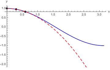
Obviously this works pretty well for x \leq 1 or so! For larger x, it starts to diverge away from cosine. We can try to improve the expansion systematically if we add more and more terms before we truncate, although we have to worry about convergence at some point.
All of this is a perfectly reasonable procedure, but it’s a little cumbersome since we have to plug in numerical values and solve. In the real world, of course, the numbers coming out of our “black box” probably also have uncertainties and we should be doing proper curve fitting, which is a topic for another class.
For our current purposes, what we really want is a way to find power-series representations when we know what f(x) is analytically, which brings us to the Taylor series.
2.4.1 Taylor series
(On notation: you may remember both the terms “Taylor series” and “Maclaurin series” as separate things. But the Maclaurin series is just a special case: it’s a Taylor series about x=0. I won’t use the separate term and will always just call this a Taylor series.)
Let’s begin with a special case, and then I’ll talk about the general idea of Taylor series expansion. Suppose we want a power-series representation for the function e^x about x=0: e^x = a_0 + a_1 x + a_2 x^2 + ... + a_n x^n + ... As we observed before, the value x=0 is special, because if we plug it in the series terminates - all the terms vanish except the first one, a_0. So we can easily find e^0 = 1 = a_0. No other value of x has this property, so it seems like we’re stuck. However, we can find a new condition by taking a derivative of both sides: \frac{d}{dx} \left( e^x \right) = a_1 + 2 a_2 x + ... + n a_n x^{n-1} + ... So if we evaluate the derivative of e^x at x=0, now the second coefficient a_1 is singled out and we can determine it by plugging in! This example is especially nice, because d/dx(e^x) gives back e^x, so: \left. \frac{d}{dx} \left( e^x \right) \right|_{x=0} = e^0 = 1 = a_1. We can keep going like this, taking more derivatives and picking off terms one by one: \frac{d^2}{dx^2} \left( e^x \right) = 2 a_2 + (3 \cdot 2) a_3 x + ... + n (n-1) a_n x^{n-2} + ... \\ \frac{d^3}{dx^3} \left( e^x \right) = (3 \cdot 2) a_3 + (4 \cdot 3 \cdot 2) a_4 x + ... + n (n-1) (n-2) a_n x^{n-2} + ... so a_2 = 1/2 and a_3 = 1/6. In fact, we can even find a_n this way: we’ll need to take n derivatives to get rid of all of the x’s on that term, and the prefactor at that point will be n(n-1)(n-2)...(3)(2) = n! So the general formula is a_n = 1/n!, and we can write out the power series in full as e^x = \sum_{n=0}^\infty \frac{x^n}{n!}. This is an example of a Taylor series expansion. A Taylor series is a power series which is obtained at a single point, by using information from the derivatives of the function we are expanding. As long as we can calculate those derivatives, this is a powerful method.
In the most general case, there are two complications that can happen when repeating what we did above for a different function. First, for most functions the derivatives aren’t all 1, and their values will show up in the power series coefficients. Second, we can expand around points other than x=0. The general form of the expansion is:
The Taylor series expansion of f(x) about the point x_0 is: f(x) = \sum_{n=0}^\infty f^{(n)}(x_0) \frac{(x-x_0)^n}{n!} \\ = f(x_0) + f'(x_0) (x-x_0) + \frac{1}{2} f''(x_0) (x-x_0)^2 + \frac{1}{6} f'''(x_0) (x-x_0)^3 + ...
Note that here I’m using the prime notation f'(x) = df/dx, and f^{(n)}(x) = d^nf/dx^n to write the infinite sum.
For most practical uses, the infinite-sum version of this formula isn’t the most useful: functions like e^x where we can calculate a general formula for all of the derivatives to arbitrarily high order are special cases. Instead, we will usually truncate this series as well. The Taylor series truncated at the (x-x_0)^n is called the n-th order series; by far the most commonly used are first order (a.k.a. linear) and second order (a.k.a. quadratic.) The names follow from the fact that these series approximate f(x) as either a linear or quadratic function in the vicinity of x_0:
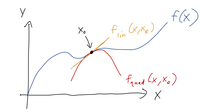
where the extra curves I drew are just the truncated Taylor series, f_{\textrm{lin}}(x,x_0) = f(x_0) + f'(x_0) (x-x_0) \\ f_{\textrm{quad}}(x,x_0) = f(x_0) + f'(x_0) (x-x_0) + \frac{1}{2} f''(x_0) (x-x_0)^2 \\
Even though we usually only need a couple of terms, one of the nice things about Taylor series is that for analytic (i.e. smooth and well-behaved) functions, which are generally what we encounter in physics, the series will always converge. So if we need to make systematic improvements to our approximation, all we have to do is calculate more terms.
Here, you should complete Tutorial 2C on “Taylor Series”. (Tutorials are not included with these lecture notes; if you’re in the class, you will find them on Canvas.)
The example below contains variations on a few things you saw on the tutorial; have a look for extra practice!
Let’s do a simple example: we’ll find the Taylor series expansion of
f(x) = \sin^2(x) up to second order. We start by calculating derivatives: f'(x) = 2 \cos (x) \sin(x) \\ f''(x) = -2 \sin^2 (x) + 2 \cos^2(x) This gives us enough to find the Taylor series to quadratic order about any point we want. For example, we can do x = \pi/4, where \cos(\pi/4) = \sin(\pi/4) = 1/\sqrt{2}. Then f'(\pi/4) = 1 \\ f''(\pi/4) = 0 and the general formula gives us \sin^2(x) \approx \frac{1}{2} + \left(x - \frac{\pi}{4} \right) + \mathcal{O}((x-\pi/4)^3) This introduces the big-O notation, which denotes order: it says that all of the missing terms are at least of order (x-\pi/4)^3, i.e. they’re proportional to (x-\pi/4)^3 or even higher powers. I’m writing it explicitly here instead of just (...), because I want to make it clear that we know the quadratic term is zero.
If we expand at x=0 instead, then \sin(0) = 0 and \cos(0) = 1 gives f'(0) = 0 \\ f''(0) = 2 and thus \sin^2(x) \approx 0 + 0 x + \frac{1}{2!} (2) x^2 + ... = x^2 + \mathcal{O}(x^3).
A couple more interesting things to point out here. First, we could have predicted that there would be no x term here: we know from the original function that \sin^2(-x) = \sin^2(x). But a linear term would be different at x and -x, so its coefficient has to be zero. In fact, this extends to all odd powers: we know in advance there will be no x^3 term, no x^5 term, and so on.
Second, notice that we would have found the same answer if we started with the Taylor expansion of \sin(x) at zero, \sin(x) \approx x - \frac{x^3}{6} + ... and just squared it: \left(x - \frac{x^3}{6} + ... \right)^2 = x^2 - \frac{1}{3} x^4 + ... \\ and up to the first two terms, we find that the expansions match.
One important note of caution here! If we use the “squaring sin(x)” trick above, there is one more term that I didn’t write down: the square of x^3/6 gives x^6 / 36. If we go back and calculate the x^6 term in the direct expansion of \sin^2(x), we’ll find this one does NOT match - the right answer is (2/45) x^6 instead! The reason for the mistake is that we’re not being consistent about the order of terms we’re keeping. \sin(x) itself has an x^5 term in the expansion, which will give another x^6 contribution: \left(x - \frac{x^3}{6} + \frac{x^5}{120} + ... \right)^2 = x^2 - \frac{1}{3} x^4 + \left(\frac{1}{36} + \frac{1}{60}\right) x^6 + ... \\ and simplifying 1/36 + 1/60 = 2/45, now we get the right answer. (But here the x^8 term will be wrong, unless we go back and add the x^7 term for \sin(x) before squaring.)
All of this is a completely general result: one way to find Taylor series for functions of functions is just to start with a simple Taylor series, and then apply other functions to it. Remember, the Taylor series is a representation of the function: f(x)^2 and \left(\sum_n (...) \right)^2 really are the same thing! We just have to be careful with keeping track of terms up to the order in x to which we want to work.
(Boas is more enthusiastic about this trick, so you can look at her chapter 1.13 for more examples. Whether it’s useful depends on the problem and on your own taste - personally I never liked polynomial long division, so I wouldn’t use this for dividing two functions!)
2.4.2 Expansion around a point, and some common Taylor series
A common situation for us in applying this to physics problems will be that we know the full solution for some system in a simplified case, and then we want to turn on a small new parameter and see what happens. We can think of this as using Taylor series to approximate f(x_0 + \epsilon) when we know \epsilon is small. This makes the expansion a pure polynomial in \epsilon, if we plug back in: f(x_0 + \epsilon) = f(x_0) + f'(x_0) \epsilon + \frac{1}{2} f''(x_0) \epsilon^2 + \frac{1}{6} f'''(x_0) \epsilon^3 + ... using x = x_0 - \epsilon, so x - x_0 becomes just \epsilon. We will prefer to write series in this form, since it’s a little simpler to write out than having to keep track of (x-x_0) factors everywhere.
There are a few very common Taylor series expansions that are worth committing to memory, because they’re used so often. We’ve seen two of them already, but I’ll include them again for easy reference:
\cos(x) \approx 1 - \frac{x^2}{2} + ... \sin(x) \approx x - \frac{x^3}{6} + ... e^x \approx 1 + x + \frac{x^2}{2} + ... \frac{1}{1+x} \approx 1 - x + x^2 + ... (1+x)^n \approx 1 + nx + \frac{n(n-1)}{2} x^2 + ...
Note that the last two are expanding the functions 1/x and x^n around 1 instead of 0, in the first case because 1/x diverges at zero. For the latter formula, if n is an integer then expanding around 0 is boring, because we already have a polynomial. However, this formula is most useful when n is non-integer. For example, we can read off the very useful result \sqrt{1+x} = (1+x)^{1/2} \approx 1 + \frac{x}{2} - \frac{x^2}{8} + ...
The (1+x)^n expansion is also known as the binomial series, because in addition to approximating functions, you can use it to work out all the terms in the expression (a+b)^n - but we won’t go into that.
I’ve mostly been letting you learn Mathematica by having you use it on homework, but finding series expansions is so useful that I’ll quickly go over how you can ask Mathematica to do it. The Mathematica function Series[] will compute a Taylor series expansion to whatever order you want. Here’s an example:
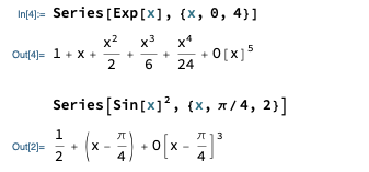
Going over the syntax: the first argument is the function you want to expand. The second argument consists of three things, collected in a list with {}: the name of the variable, the expansion point, and the maximum order that you want.
Find the Taylor series expansion of \ln(1+x) to third order about x=0.
If you’re following along at home, try it yourself before you keep reading! This is the key piece that we’ll need to go back and finish our projectiles with air resistance calculation.
Answer:
Following the \epsilon version of the formula above, we can write this immediately as a Taylor series in x if we expand about 1. If we define f(u) = \ln(u) (changing variables to avoid confusion), then expanding about u_0 = 1 gives f(1+x) = f(1) + f'(1) x + \frac{1}{2} f''(1) x^2 + \frac{1}{3!} f'''(1) x^3 + ... (since u - u_0 = (1+x) - 1 = x.) This is nice because it skips right to what we want, an expansion in the small quantity x, but using the slightly simpler function \ln(u). If you instead took derivatives of \ln(1+x) in x directly, that’s fine too - you’ll get the same series.
Now we need the derivatives of \ln(u): f'(u) = \frac{1}{u} f''(u) = -\frac{1}{u^2} f'''(u) = \frac{2}{u^3} so f'(1) = 1, f''(1) = -1, and f'''(1) = 2. Finally, we plug back in to find: \ln(1+x) \approx x - \frac{1}{2} x^2 + \frac{1}{3} x^3 + ...
Notice that this formula is also valid for negative values of x, so if we want to expand \ln (1-x), we just flip the sign, i.e. \ln(1-x) \approx -\left(x + \frac{x^2}{2} + \frac{x^3}{3} + ... \right)
2.4.3 Back to linear air resistance
This ends our important and lengthy math detour: let’s finally go back and finish discussing projectile motion with linear air resistance. Our stopping point was the formula for the trajectory,
y(x) = v_{\textrm{ter}} \tau \ln \left( 1 - \frac{x}{\tau v_{x,0}} \right) + \frac{v_{y,0} + v_{\textrm{ter}}}{v_{x,0}} x where v_{\textrm{ter}} = mg/b and \tau = m/b. We’d like to understand what happens as b becomes very small, where we should see this approach the usual “vacuum” result of parabolic motion. One option would be to plug the explicit b-dependence back in and series expand in that, but that will be messy for two reasons: there are b’s in several places, and b is a dimensionful quantity (units of force/speed = N \cdot s / m, remember.)
Strictly speaking, we should never Taylor expand in quantities with units, because the whole idea is to expand in a small parameter, but if it has units we have to answer the question “small compared to what?” to see if our series is working or not.
If you do Taylor expand in something dimensionful, nothing terrible will happen; as long as you do the math correctly, the units will be compensated by other constants that appear in the expansion. You can try it on this example; expanding around b = 0 should lead you to the same answer. But it is harder to tell if the expansion is justified or not if you expand in something with units!
Both problems can be solved by noticing that the combination \frac{x}{\tau v_{x,0}} = \frac{xb}{mv_{x,0}} is dimensionless, and definitely small as b \rightarrow 0 with everything else held fixed. This only appears in the logarithm, but the logarithm is the only thing we need to series expand anyway.
With that setup, let’s apply our result for \ln(1+\epsilon) above, setting \epsilon = \frac{x}{\tau v_{x,0}}. We find: y(x) \approx v_{\textrm{ter}} \tau \left[ -\frac{x}{\tau v_{x,0}} - \frac{x^2}{2\tau^2 v_{x,0}^2} - \frac{x^3}{3\tau^3 v_{x,0}^3} + ... \right] + \frac{v_{y,0} + v_{\textrm{ter}}}{v_{x,0}} x We immediately spot that the very first term and the very last term are equal and opposite, so they cancel each other: y(x) \approx \frac{v_{y,0}}{v_{x,0}} x - v_{\textrm{ter}} \tau \left[ \frac{x^2}{2\tau^2 v_{x,0}^2} + \frac{x^3}{3\tau^3 v_{x,0}^3} + ... \right]
As b \rightarrow 0, we know that v_{\textrm{ter}} is becoming very large. This might make you worry about the v_{\textrm{ter}} \tau appearing outside the square brackets, but remember that \tau is becoming large too, and we have some \tau factors in the denominator. In fact, we can go back to the definitions to notice that \frac{v_{\textrm{ter}}}{\tau} = \frac{mg/b}{m/b} = g which we can use to continue simplifying: y(x) \approx \frac{v_{y,0}}{v_{x,0}} x - \frac{x^2 g}{2v_{x,0}^2} - \frac{x^3 g}{3 \tau v_{x,0}^3} + ... There’s the quadratic term in x, which no longer depends on anything to do with air resistance! In fact, now that we’ve simplified we can take b \rightarrow 0 completely, which will make \tau \rightarrow \infty and the third term vanish. This kills all of the higher terms in the expansion as well, leaving us with y_{\textrm{vac}}(x) = \frac{v_{y,0}}{v_{x,0}} x - \frac{x^2 g}{2v_{x,0}^2}. This is, in fact, exactly the formula you’ll find in your freshman physics textbook for projectile motion with no air resistance. Limit checked successfully!
Better still, we now have a nice approximate formula that we can use in cases where the air resistance is relatively small. (Explicitly, “small” in that we only consider values of x \ll \tau v_{x,0}.) So long as this condition is satisfied, we see that we have a correction term for the vacuum trajectory which is of order x^3. For positive x this term is always negative, so the projectile will fall more quickly than it would in vacuum, matching our intuition that the drag force will slow down and hinder the projectile’s motion.
As a last step, let’s take our results and find the range R, which is what Taylor focuses on in his discussion. The range is the value of x (not at zero) for which y=0. This is easily found for the vacuum solution: y_{\textrm{vac}}(R) = 0 = \frac{v_{y,0}}{v_{x,0}} R - \frac{g}{2v_{x,0}^2} R^2 = R \left( \frac{v_{y,0}}{v_{x,0}} - \frac{g}{2v_{x,0}^2} R \right) \\ \Rightarrow R_{\textrm{vac}} = \frac{2 v_{x,0} v_{y,0}}{g}.
Now with drag turned on and including the cubic term, we get a quadratic equation: 0 = \frac{v_{y,0}}{v_{x,0}} R - \frac{g}{2v_{x,0}^2} R^2 - \frac{g}{3\tau v_{x,0}^3} R^3 + ... which, moving the R^2 term to the left and canceling one R off, we can rearrange as R = \frac{2 v_{x,0} v_{y,0}}{g} - \frac{2}{3\tau v_{x,0}} R^2.
The second term here is proportional to the combination R/(\tau v_{x,0}), which is the small parameter we expanded in for the case of small drag. Thus, as b \rightarrow 0 the second term will go away and just leave the first term - which is just the vacuum result, once again.
However, we don’t want to just completely throw away the second term - we want to know the leading correction due to the presence of air resistance. To do that, let’s assume that the correction is small compared to the vacuum range: we write R = R_{\textrm{vac}} + \delta R + ... where \delta R \ll R_{\textrm{vac}}. The (…) reminds us that this is implicitly an expansion in R/(\tau v_{x,0}), from which we’re just keeping the first b-dependent term. We can plug this back in to our quadratic equation: R_{\textrm{vac}} + \delta R = R_{\textrm{vac}} - \frac{2}{3\tau v_{x,0}} (R_{\textrm{vac}} + \delta R)^2 using the fact that we recognize the vacuum range as the first term on the right-hand side. Now, we can expand out the square on the right: \delta R = -\frac{2}{3\tau v_{x,0}} \left( R_{\textrm{vac}}^2 + 2 R_{\textrm{vac}} \delta R \right) where we throw away the (\delta R)^2 piece, because it’s much smaller than everything else in the equation. (More properly, it’s a higher-order piece in the expansion, so we shouldn’t keep if it we’ve decided to work at first order.)
We can continue by solving for \delta R, but we’ll save a bit of work if we stop and think carefully about what terms we should keep. In particular, remember that R_{\textrm{vac}} / (\tau v_{x,0}) is a small expansion parameter. Since the entire right-hand side is proportional to this small quantity, we should also throw away the R_{\textrm{vac}} \delta R term, since it’s also second-order as the air resistance goes to zero. That leaves us with the result: \delta R = -\frac{2R_{\textrm{vac}}^2}{3\tau v_{x,0}} = -R_{\textrm{vac}} \frac{4 v_{y,0}}{3 \tau g} = -R_{\textrm{vac}} \frac{4 v_{y,0}}{3 v_{\textrm{ter}}}. Plugging back in, we find our full result for the range at first order with air resistance, R \approx R_{\textrm{vac}} \left( 1 - \frac{4 v_{y,0}}{3 v_{\textrm{ter}}} \right).
This is a small correction to the range so long as v_{y,0} \ll v_{\textrm{ter}}. If v_{y,0} is close to v_{\textrm{ter}}, this would be a large correction, but then we’re also approaching the situation where our approximation is breaking down and we can’t trust this result anymore!
You might wonder, what happens if we just solve the quadratic equation above for R instead of doing the expansion R = R_{\textrm{vac}} + \delta R? We will get exactly the same answer - as long as we’re careful about how we treat higher-order terms in our series. Details are in the aside below for the curious.
I want to make one last point regarding series expansion and working to a certain order, before we move on to the next physics problem. Instead of doing the manipulations I did above and introducing the new variable \delta R, it would have been perfectly valid to solve the quadratic equation for R instead, 0 = \frac{v_{y,0}}{v_{x,0}} - \frac{g}{2v_{x,0}^2} R - \frac{g}{3\tau v_{x,0}^3} R^2 + ... What if we just plug this in to the quadratic formula? The positive solution turns out to be: R = -\frac{3}{4} v_{x,0} \tau + \frac{\sqrt{3 \tau} v_{x,0}}{4g} \sqrt{3g^2 \tau + 16g v_{y,0}}. This looks messy, and also doesn’t look even remotely like the result we found above! Why is this equation so different? The short answer is that we have to remember that we’re working with a series expansion as b \rightarrow 0, and therefore in \tau \rightarrow \infty. So we have to expand out functions like square roots involving \tau, and just keep the leading terms, or else we’re fooling ourselves!
I won’t try to do this by hand, because the algebra is a little messy, but we can use Mathematica to carry out the expansion for us at \tau = \infty:
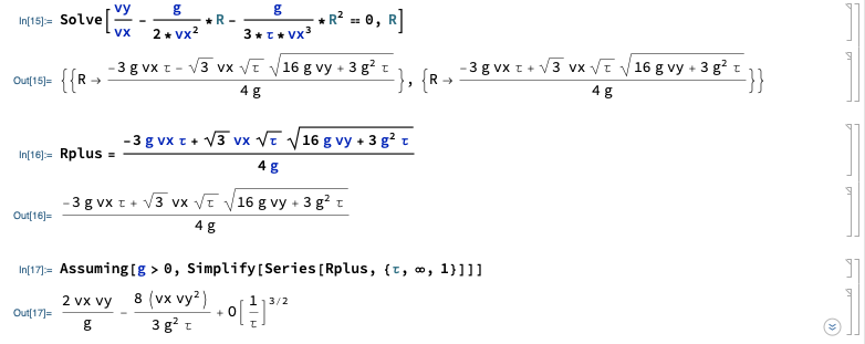
Tricks of the trade: the Assuming[] statement makes the answer look nicer, otherwise you’ll end up with things like \sqrt{g^2} / g which Mathematica will refuse to cancel off, assuming g might be negative. Also, notice that we can series expand directly at infinity: type Esc-i-n-f-Esc as a shortcut to write the infinity symbol. If you were doing this by hand, you would instead want to define \epsilon = 1/\tau and then expand at \epsilon = 0.
Having worked out the algebra, we have our result, which we can write most clearly by factoring out the vacuum range: R = \frac{2v_{x,0} v_{y,0}}{g} \left( 1 - \frac{4v_{y,0}}{3g\tau} \right) = R_{\textrm{vac}} \left( 1 - \frac{4v_{y,0}}{3v_{\textrm{ter}}} \right), matching what we had before.
2.5 Quadratic drag
Let’s turn to purely quadratic air resistance now: \vec{f}(v) = -cv^2 \hat{v} As a reminder, this will be an accurate model for situations in which cv^2 \gg bv, or equivalently when the Reynolds number R = D \rho v / \eta is much larger than 1. For most everyday objects moving at normal speeds, R \gg 1 and the quadratic model is the one which applies. (However, as I’ll emphasize again later, if v is too small the quadratic drag is vanishing, so we have to be careful if our object is coming to a stop!)
Following the linear case study, I’ll start with horizontal motion. For an object moving purely in the +\hat{x} direction subject to quadratic drag, and no other forces, we have the equation of motion m \ddot{x} = -c \dot{x}^2. Written in terms of v_x this is a separable first-order ODE; in fact, it’s one we solved as an exercise back when we were talking about ODEs in general. The solution we found was v(t) = \frac{v_0}{1 + \frac{cv_0}{m} t} = \frac{v_0}{1 + t/\tau_c}, defining the quadratic natural time \tau_c = \frac{m}{cv_0}. (Notation break from Taylor: he just calls this \tau as well. I wanted to label it clearly as different from the linear version.)
Checking units is a good habit, so let’s make sure this is indeed a time. c must have units of force over speed squared, or N \cdot s^2 / m^2, which means cv_0 is in N \cdot s / m = kg / s using the definition of a Newton (which is easy to remember since \vec{F} = m\vec{a}.) The mass up top cancels the kg, leaving s, so indeed this is a time. Specifically, we see that t=\tau_c is the time at which the initial speed is halved, v(\tau_c) = \frac{v_0}{2}. To avoid confusion, notice that this is not the same as a half-life that would appear in radioactive decay! In particular, v(2\tau) = v_0 / 3, whereas if we waited for two half-lives we would expect to have 1/2^2 = 1/4 of our initial sample remaining. The difference is that our solution v(t) is not exponential in time, but instead dies off much more slowly as t \rightarrow \infty.
What about position as a function of time? We can obtain that just by integrating once, as always: x(t) = x_0 + \int_0^t dt' v(t') \\ = x_0 + \int_0^t dt' \frac{v_0}{1+t'/\tau_c} \\ = x_0 + v_0 \tau_c \ln \left( 1 + \frac{t}{\tau_c} \right).
Here are a couple of sketches of the time dependence, before we discuss further:
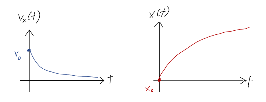
You may remember in the linear drag case that the x position approached a finite asymptotic value x_\infty as our object came to a stop. That’s not true in this case: the logarithm actually never stops growing with t, so \lim_{t \rightarrow \infty} x(t) = \infty! This is because as we already noted, in the quadratic case, the speed v(t) decreases more slowly with time.
This might seem really weird, because we seem to be concluding that a moving object under the effects of quadratic drag can travel infinitely far without stopping - and this is the case that is appropriate for everyday objects! The key point to remember is that this model will inevitably become invalid when v(t) becomes small enough: as the quadratic drag force becomes smaller, eventually some other force (linear drag, or friction) will be large enough that we can’t ignore it anymore.
Taylor gives the nice example of a person riding a bicycle, coasting to a stop from a fairly high speed. Our quadratic drag model for x(t) will describe this motion well for a while, but eventually as the bicycle slows down, ordinary friction between the wheels and the ground will become large enough to notice, bringing it to a stop in a finite distance. (Linear drag could do the same thing, but it so happens that friction is stronger for the bicycle case.)
2.5.1 Vertical motion with quadratic drag
Now let’s look at vertical motion, which means turning on gravity. For our solution we will follow Taylor and only consider the case where the object is moving downwards, v_y < 0 in my notation, in which case \dot{v}_y = -g + \frac{c}{m} v_y^2\ \ (v_y < 0).
(The opposite-sign case v_y > 0 is discussed briefly in the context of terminal velocities above.) As a reminder, this solution has a terminal velocity v_{{\textrm{ter}}, c} = \sqrt{\frac{mg}{c}}. Once again, we have an inhomogeneous ODE. Even worse, this is actually a non-linear ODE because of the square! That means that we can’t attack it using the complementary + particular solution method - we’ll get the wrong answer if we try.
The good news is that we can still get a general solution because the ODE is still separable. Dividing the right-hand side out, \frac{\dot{v}_y}{-g+\frac{c}{m} v_y^2} = 1 \\ \frac{dv_y}{1 - v_y^2 / v_{{\textrm{ter}},c}^2 } = -g dt where I plugged in the terminal velocity to make things look nicer. Now integrating and doing a quick variable change, v_{{\textrm{ter}}, c} \int \frac{du}{1-u^2} = -\int g dt where u = v_y / v_{{\textrm{ter}},c}. This is a very standard integral, and it’s easy to look up the result - in fact, it’s in the front cover of Taylor: \int \frac{du}{1-u^2} = \tanh^{-1}(u). \tanh^{-1} is the inverse hyperbolic tangent function (pronounced “tanch-inverse” or “arc-tanch”). If you’re familiar with hyperbolic trig functions, then this is a useful answer, but if you’re not then it isn’t!
In fact, you can do this integral without any fancy new functions, just by expansion in partial fractions. Since this is a method you should have seen already, I’m going to put the details in an optional aside.
You may remember from your calculus class that a good trick to deal with integrals of rational functions is to split them up into separate terms. Here, we notice that \frac{1}{1-u^2} = \frac{1}{(1+u)(1-u)} = \frac{1/2}{1+u} + \frac{1/2}{1-u}. With the integrand split apart, we’re left with two integrals that we know how to do: \int du\ \left( \frac{1/2}{1+u} + \frac{1/2}{1-u} \right) = \frac{1}{2} \ln (1+u) - \frac{1}{2} \ln (1-u) \\ = \frac{1}{2} \ln \left( \frac{1+u}{1-u} \right). Back to our full equation, we have \frac{1}{2} \ln \left( \frac{1+u}{1 - u} \right) = -\frac{gt}{v_{{\textrm{ter}},c}} + A\\ \frac{1+u}{1 - u} = B e^{-2gt / v_{{\textrm{ter}},c}} keeping track of our arbitrary constant of integration. Before we continue, notice that we can once again define a natural time in freefall from the terminal velocity in the same way as the linear case, \tau \equiv \frac{v_{\textrm{ter},c}}{g}. (not the same as \tau_c above, beware!) I’ll use \tau from this point on to save some writing. The last step is to solve for v_y, which means solving for u. If we begin by multiplying through to get rid of the fraction, 1+u = Be^{-2t/\tau} (1-u) \\ u (1 + Be^{-2t/\tau}) = Be^{-2t/\tau} - 1 so plugging in u = v_y / v_{{\textrm{ter}}, c}, v_y(t) = v_{{\textrm{ter}},c} \frac{Be^{-2t/\tau} - 1}{Be^{-2t/\tau} + 1}. Finally, we need to fix the constant of integration. Let’s take v_y(0) = -v_0, where v_0 like v_{{\textrm{ter}},c} is a positive speed. Then we have -v_0 = v_{{\textrm{ter}},c} \frac{B-1}{B+1} \Rightarrow B = \frac{v_{{\textrm{ter}},c} + v_0}{v_{{\textrm{ter}},c} - v_0}. In the special case that we start from rest, v_0 = 0, then B = 1 and our solution is v_y(t) = v_{{\textrm{ter}},c} \frac{e^{-2t/\tau} - 1}{e^{-2t/\tau} + 1}.
The final result in the aside above is, for starting from rest (v_0 = 0), v_y(t) = v_{{\textrm{ter}},c} \frac{e^{-2gt/v_{\textrm{ter}, c}} - 1}{e^{-2gt/v_{\textrm{ter},c}} + 1}.
Physics first: notice that the exponential pieces are always less than 1, so the fraction is always negative, which it had better be because we assumed v_y < 0! As t \rightarrow \infty, the exponentials vanish, and we approach the terminal velocity asymptotically, like in the linear case.
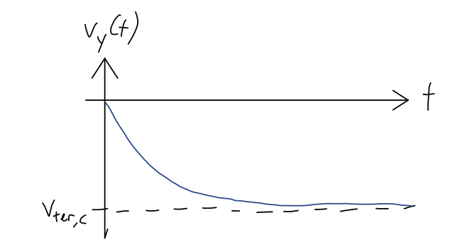
Although this doesn’t need any hyperbolic functions, the solution above for v_y(t) is actually an example of one! Let’s do a quick review of hyperbolic functions in order to recognize it.
2.5.2 Interlude: hyperbolic trig functions
As the result above hints, hyperbolic trig functions are combinations of exponentials, e^{\pm x}. We begin with the definitions of hyperbolic sine and cosine: \sinh(x) = \frac{1}{2} (e^x - e^{-x}) \cosh(x) = \frac{1}{2} (e^x + e^{-x}) An easy way to remember which one has the minus sign: \sinh(x) is odd, just like \sin(x). At large negative and positive x, these are dominated by one or the other exponential. So the whole functions resemble two exponential curves stuck together, with or without a minus sign:
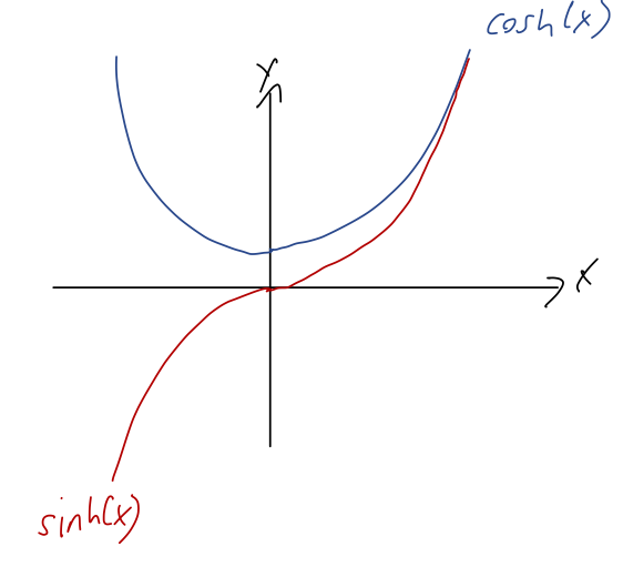
The reason these are called hyperbolic trig functions is that they satisfy a number of identities that are similar to the regular trig identities: for example, \cosh^2 x - \sinh^2 x = 1. (Actually, the real reason is because you can define them by trying to do trigonometry using a unit hyperbola instead of a unit circle, and the deeper reason is that they’re actually related to ordinary trig functions once you start using complex numbers.)
Finally, the hyperbolic tangent is defined in analogy to the regular tangent: \tanh(x) = \frac{\sinh(x)}{\cosh(x)} =\frac{e^x - e^{-x}}{e^x + e^{-x}} = \frac{e^{2x} - 1}{e^{2x} + 1}. Here’s a sketch of that function, showing the asymptotes at \pm 1:
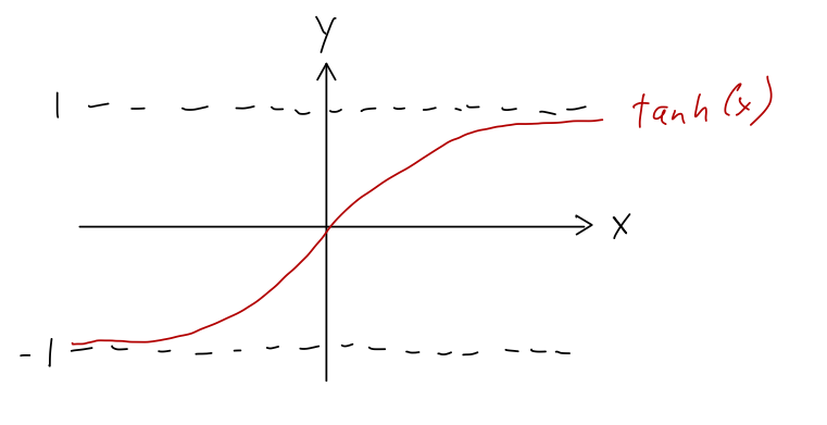
This function comes up frequently in physics - we’ve just seen an example - but the fact that it smoothly goes from -1 to +1 makes it useful in a variety of engineering applications as well, because it maps an arbitrary input signal into a finite range. One example is in machine learning, where the response of individual neurons in a neural net is often modeled with \tanh.
That’s all there is to hyperbolic trig! Again, there are a number of “trig identities” we can apply, but there’s no reason for me to go over those here - like the ordinary identities for sin, cos, and tan, you look those up when you need them. But now, returning to our solution starting at rest: v_y(t) = v_{{\textrm{ter}},c} \frac{e^{-2gt/v_{\textrm{ter}, c}} - 1}{e^{-2gt/v_{\textrm{ter},c}} + 1}. we see that can we write our solution simply as a hyperbolic tangent: v_y(t) = -v_{{\textrm{ter}},c} \tanh \left( \frac{gt}{v_{{\textrm{ter}},c}} \right).
The \tanh formula above is nice and simple, but it’s also only true if we start at rest! For v_0 \neq 0, the general solution can be readily found from our results above: v_y(t) = v_{{\textrm{ter}},c} \frac{(v_{{\textrm{ter}},c} + v_0) e^{-2gt/v_{\textrm{ter},c}} - (v_{{\textrm{ter}},c} - v_0)}{(v_{{\textrm{ter}},c} + v_0) e^{-2gt/v_{\textrm{ter},c}} + (v_{{\textrm{ter}},c} - v_0)}. You can still technically write this as a hyperbolic tangent, but the result is not very nice looking: v_y(t) = -v_{\textrm{ter}, c} \tanh \left( \frac{gt}{v_{\textrm{ter}, c}} - \tanh^{-1} \left( \frac{v_0}{v_{\textrm{ter}, c}} \right) \right).
This is a good reminder that it’s important to carry your integration constants along when solving ODEs! If you just solved at rest, you might be tempted to think that the general solution for a moving initial condition would just be to add v_0 to the \tanh(...) solution above - but that would be wrong!
One final thing to point out, linking back to our general discussion of ODEs. Remember that this is a non-linear ODE, for which we were warned that we can’t necessarily find a general solution. What we just found looks general, but don’t forget that we had to assume v_y < 0. If instead we had taken v_y > 0, a very important minus sign would be flipped, and the key integral above would become \int \frac{du}{1+u^2} = \tan^{-1}(u). So solutions for positive initial speed look like regular tangent instead of hyperbolic tangent. In other words, the functional form of our solution changes depending on initial conditions! This is always a possibility if our ODE is non-linear.
Here, you should complete Tutorial 2D on “Velocity-dependent forces - part 2”. (Tutorials are not included with these lecture notes; if you’re in the class, you will find them on Canvas.)
Let’s run a detailed example now, to tie together everything we’ve been thinking about!
I accidentally drop my wedding ring (mass ~ 10 g, width ~ 6 mm) into a glass of dark beer. Beer is more viscous than air, by a factor of about 137 according to Wikipedia; it’s also more dense than air, by a factor of about 750.
- Is linear or quadratic drag dominant?
- What is the terminal velocity?
- How long will it take to hit the bottom of a 15-cm tall pint glass, using a first-order series expansion? Is this result trustworthy?
Starting with part a), I know how the drag coefficients scale with viscosity and density, \beta = 3\pi \eta,\ \ \gamma = \frac{1}{2} C_D \rho (A/D^2). The important part is that \beta is linear in the viscosity \eta, and \gamma is linear in medium density \rho. Comparing to air as a baseline, the density goes up more than the viscosity does, so \gamma will increase more than \beta. Because we know that everyday objects tend to be quadratic-drag dominated in air, this will probably still be true in the beer, so this should be a quadratic drag problem.
Just to be thorough, I’ll calculate both drag coefficients, using Taylor’s values for air and D = 6 mm: b = \beta_{\textrm{air}} \frac{\eta_{\textrm{beer}}}{\eta_{\textrm{air}}} D \\ = (1.6 \times 10^{-4}\ {\textrm{N}} \cdot {\textrm{s}} / {\textrm{m}}^2) (137) (6\times 10^{-3}\ {\textrm{m}}) \\ = 1.3 \times 10^{-4}\ {\textrm{N}} \cdot {\textrm{s}} / {\textrm{m}} and c = \gamma_{\textrm{air}} \frac{\rho_{\textrm{beer}}}{\rho_{\textrm{air}}} D^2 \\ = (0.25\ {\textrm{N}} \cdot {\textrm{s}}^2 / {\textrm{m}}^4) (750) (6 \times 10^{-3}\ {\textrm{m}})^2 \\ = 6.8 \times 10^{-3}\ {\textrm{N}} \cdot {\textrm{s}}^2 / {\textrm{m}}^2. So the Reynolds number is R = \frac{cv}{b} = \frac{v}{0.019\ {\textrm{m}}/{\textrm{s}}}.
As long as the terminal velocity for quadratic drag isn’t too close to 0.019\ {\textrm{m}}/{\textrm{s}}, then, we expect the quadratic force to dominate.
On to part b), which is simple: we just plug in to the formula for quadratic freefall and find v_{\textrm{ter},c} = \sqrt{\frac{mg}{c}} = \sqrt{\frac{(10^{-2}\ {\textrm{kg}})(9.8\ {\textrm{m}}/{\textrm{s}}^2)}{6.8 \times 10^{-3}\ {\textrm{N}} \cdot {\textrm{s}}^2 / {\textrm{m}}^2}} \approx 3.8\ {\textrm{m}}/{\textrm{s}}. This is safely large enough that our Reynolds number will be very large for the majority of the motion, so the quadratic model is okay. For good measure, we should also calculate the natural time: \tau = \frac{g}{v_{\textrm{ter},c}} = 2.6\ {\textrm{s}}.
Finally, we ask about series expansion of the answer - although we know the full solution in this case, it’s still useful to think about to improve our understanding of series expansion use in general. As we just found, the full solution starting from rest is v_y(t) = -v_{\textrm{ter},c} \tanh \left( \frac{t}{\tau} \right)
We could look up a formula for the series expansion of \tanh, or look up its derivatives and expand ourselves, but I’ll use a trick to find the expansion to first order instead. Recall the definition: \tanh(x) = \frac{e^{2x} - 1}{e^{2x} + 1} Now I’ll apply the series expansions for e^{2x}: \tanh(x) = \frac{1 + 2x + 2x^2 + ... - 1}{1 + 2x + 2x^2 + ... + 1} = \frac{x+...}{1+x+...} cancelling off a 2. We’re still not finished, since this isn’t a polynomial yet. But we can use the expansion 1/(1+x) = 1-x + ... to move the denominator up top, \tanh(x) = (x+...) (1 - x + ...) = x + \mathcal{O}(x^2) Actually, there is no \mathcal{O}(x^2) term at all, because of the relation \tanh(-x) = -\tanh(x). So the missing terms start at \mathcal{O}(x^3). From this expansion, we have v_y(t) \approx -v_{\textrm{ter},c} \frac{t}{\tau} and then y(t) \approx \int_0^t\ v_y(t')\ dt' = -\frac{v_{\textrm{ter},c} t^2}{2\tau} \\ \Rightarrow t = \sqrt{\frac{2h\tau}{v_{\textrm{ter},c}}} where h is the drop height. Plugging in numbers gives t \approx 0.45 s.
Now, the final question: do I trust the series expansion result? This is a question about error due to series expansion, usually we would state the condition to use the expansion as “t \ll \tau”. But let’s be more precise. By using a series expansion, the error we’re making is roughly the size of the first missing term in the expansion, which is proportional to (t/\tau)^3. If we had kept that term, our formula for v_y(t) would have been v_y(t) \approx -v_{\textrm{ter},c} \frac{t}{\tau} \left(1 + K \frac{t^2}{\tau^2} \right), where to figure out K we’d have to compute the Taylor expansion out to third order. If we really want to be careful, we can do just that, but instead let’s assume K is not too far from 1. Then what matters is the size of t^2/\tau^2, which is \frac{t^2}{\tau^2} \approx 0.03. So, up to the size of whatever the number K turns out to be, we’re making an error of around 3% in v_y(t) by using the first-order series expansion. The first observation we can make is that since this is much smaller than 1, we don’t have to worry about convergence of the series, i.e. the first-order answer is a good initial guess.
Beyond that, do we need to go find the next term in the expansion? If I’m just observing this process happening by eye, then probably not; I don’t think a human observer would easily notice differences on the order of a few hundredths of a second. On the other hand, if I want to know the answer to within 1% accuracy - maybe if I want to make measurements of this kind of motion to work backwards and calculate the density of the beer, for example - then I do need to keep the next term in the series.
To summarize: the order at which we stop is always found by the accuracy at which we need the answer; and (as long as the series converges!) we can always get better accuracy by continuing the expansion to the next order.
2.5.3 Projectiles with quadratic resistance; linear + quadratic resistance
At this point, the obvious next step would be to try to put our solutions together to study projectile motion with quadratic drag. Unfortunately, there’s an obstacle to doing this that wasn’t present in the linear case, which we can see if we go back to the vector form of Newton’s second law. In the linear case, we have \vec{F} = m\dot{\vec{v}} = m\vec{g} - bv \hat{v} = m\vec{g} - b\vec{v}. This splits cleanly into two separate equations for v_x and v_y, because only \vec{v} appears on both sides. However, in the quadratic case, the general equation is m\dot{\vec{v}} = m\vec{g} - cv^2 \hat{v} = m\vec{g} - cv \vec{v}. This almost splits up in the same way, but we have an extra factor of v, which is the overall speed. If we write this full equation out in components, we find \dot{v}_x = -\frac{c}{m} \sqrt{v_x^2 + v_y^2} v_x \\ \dot{v}_y = -g - \frac{c}{m} \sqrt{v_x^2 + v_y^2} v_y. These are non-linear ODEs, but even worse they’re coupled ODEs, meaning that we have to solve them simultaneously because each equation depends on the other unknown velocity component. In fact, the only way we can deal with these more complicated equations is to solve them numerically. Taylor talks a little bit about this, but I’ll let you read his example and will not say any more here.
We run into a similar problem if we try to solve the general case of having both linear and quadratic drag forces, m\dot{\vec{v}} = m\vec{g} - b\vec{v} - cv \vec{v} which would be required when the Reynolds number is close to 1. It is actually possible to solve the horizontal- and vertical-motion cases analytically here, but those full solutions won’t show off anything new and interesting in terms of either physics or math, so we’ll skip over them. The full study of projectile motion with both terms can only be done numerically due to the quadratic term.