5 Harmonic oscillators
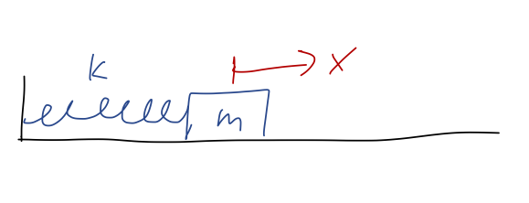
The big physics topic of this chapter is something we’ve already run into a few times: oscillatory motion, which also goes by the name harmonic motion. This sort of motion is given by the solution of the simple harmonic oscillator (SHO) equation, m\ddot{x} = -kx This happens to be the equation of motion for a spring, assuming we’ve put our equilibrium point at x=0:
The simple harmonic oscillator is an extremely important physical system study, because it appears almost everywhere in physics. In fact, we’ve already seen why it shows up everywhere: expansion around equilibrium points. If y_0 is an equilibrium point of U(y), then series expanding around that point gives U(y) = U(y_0) + \frac{1}{2} U''(y_0) (y-y_0)^2 + ... using the fact that U'(y_0) = 0, true for any equilibrium. If we change variables to x = y-y_0, and define k = U''(y_0), then this gives U(x) = U(x_0) + \frac{1}{2} kx^2 and then F(x) = -\frac{dU}{dx} = -kx which results in the simple harmonic oscillator equation. Since we’re free to add an arbitrary constant to the potential energy, we’ll ignore U(x_0) from now on, so the harmonic oscillator potential will just be U(x) = (1/2) kx^2.
Before we turn to solving the differential equation, let’s remind ourselves of what we expect for the general motion using conservation of energy. Suppose we have a fixed total energy E somewhere above the minimum at E=0. Overlaying it onto the potential energy, we have:
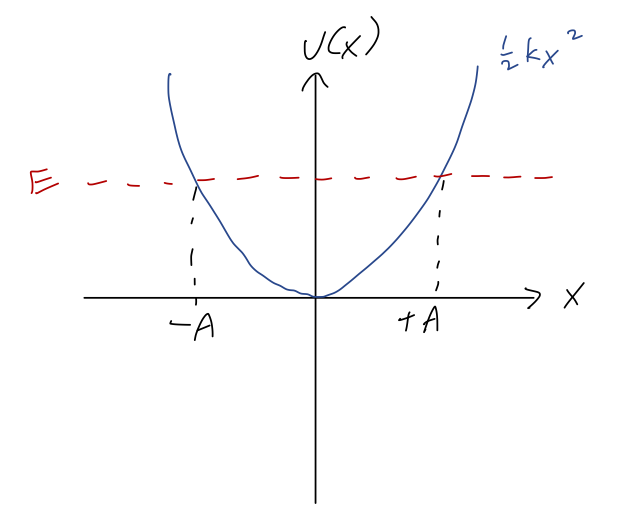
Because of the symmetry of the potential, if the value of x where E = U at positive x is U(A) = E, then we must also have U(-A) = E. Since these are the turning points, we see that A, the amplitude, is the maximum possible distance that our object can reach from the equilibrium point; it must oscillate back and forth between x = \pm A. We also know that T=0 at the turning points, which means that E = \frac{1}{2} kA^2.
This relation will make it useful to write our solutions in terms of the amplitude. But to do that, first we have to find the solutions! It’s conventional to rewrite the SHO equation in the form \ddot{x} = -\omega^2 x, where \omega^2 \equiv \frac{k}{m}. The combination \omega has units of 1/time, and the notation suggests it is an angular frequency - we’ll see why shortly.
5.1 Solving the simple harmonic oscillator
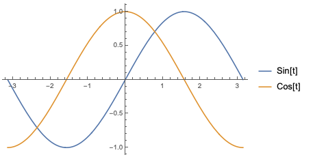
I’ve previously argued that just by inspection, we know that \sin(\omega t) and \cos(\omega t) solve this equation, because we need an x(t) that goes back to minus itself after two derivatives (and kicks out a factor of \omega^2.) But let’s be more systematic this time.
Thinking back to our general theory of ODEs, we see that this equation is:
- Linear (no functions acting on x)
- Second-order (double derivative on the left-hand side)
- Homogeneous (every term has an x or derivatives)
Since it’s linear, we know there exists a general solution, and since it’s second-order, we know it must contain exactly two unknown constants. We haven’t talked about the importance of homogeneous and second-order yet, so let’s look at that now. The most general possible homogeneous, linear, second-order ODE takes the form \frac{d^2y}{dx^2} + P(x) \frac{dy}{dx} + Q(x) y(x) = 0, where P(x) and Q(x) are arbitrary functions of x. All solutions of this equation for y(x) have an extremely useful property known as the superposition principle: if y_1(x) and y_2(x) are solutions, then any linear combination of the form ay_1(x) + by_2(x) is also a solution. It’s easy to show that if you plug that combination in to the ODE above, a bit of algebra gives a \left( \frac{d^2y_1}{dx^2} + P(x) \frac{dy_1}{dx} + Q(x) y_1(x) \right) + b \left( \frac{d^2y_2}{dx^2} + P(x) \frac{dy_2}{dx} + Q(x) y_2(x) \right) = 0 and since by assumption both y_1 and y_2 are solutions of the original equations, both of the expressions in parentheses are 0, so the whole left-hand side is 0 and the equation is true. Notice that the homogeneous part is very important for this: if there was some other F(x) on the right-hand side of the original equation, then we would get aF(x) + bF(x) on the left-hand side for our linear combination, and superposition will not work.
Anyway, the superposition principle greatly simplifies our search for a solution: if we find any two solutions, then we can add them together with arbitrary constants and we have the general solution. Let’s go back to the SHO equation: \ddot{x} = - \omega^2 x As I mentioned before, two functions that both satisfy this equation are \sin(\omega t) and \cos(\omega t). So the general solution, by superposition, is x(t) = B_1 \cos (\omega t) + B_2 \sin (\omega t).
For a general solution, we have to verify that the solutions we are adding together are linearly independent. This means simply that if we have two functions f(x) and g(x), there is no solution to the equation k_1 f(x) + k_2 g(x) = 0 except for k_1 = k_2 = 0. If there was such a solution, then we could solve for one of the functions in terms of the other, for example g(x) = -(k_1/k_2) f(x). This solution means that the linear combination C_1 f(x) + C_2 g(x) is really just the same as a single constant multiplying f(x).
If you’re uncertain about whether a collection of functions are linearly independent or not, there’s a simple test that you can do using what is known as the Wronskian determinant. For our present purposes we don’t really need the Wronskian - we know enough about trig functions to test for linear independence directly. If you’re interested, have a look at Boas 3.8.
Now, back to our general solution: x(t) = B_1 \cos (\omega t) + B_2 \sin (\omega t).
This is indeed oscillatory motion, since both \sin and \cos are periodic functions: specifically, if we wait for t = \tau = 2\pi / \omega, then x(t+\tau) = B_1 \cos (\omega t + 2\pi) + B_2 \sin (\omega t + 2\pi) = B_1 \cos (\omega t) + B_2 \sin (\omega t) = x(t) i.e. after a time of \tau, the system returns to exactly where it was. The time length \tau = \frac{2\pi}{\omega} is known as the period of oscillation, and we see that indeed \omega is the corresponding angular frequency.
To fix the arbitrary constants, we would just need to plug in initial conditions. If we have an initial position x_0 and initial speed v_0, then plugging in at t=0 the sine always vanishes, and we get the simple system of equations x_0 = x(0) = B_1 \\ v_0 = \dot{x}(0) = B_2 \omega so x(t) = x_0 \cos (\omega t) + \frac{v_0}{\omega} \sin (\omega t). This is a perfectly good solution, but this way of writing it makes answering certain questions inconvenient. For example, what is the amplitude A, i.e. the maximum displacement from x=0? It’s possible to solve for, but certainly not obvious.
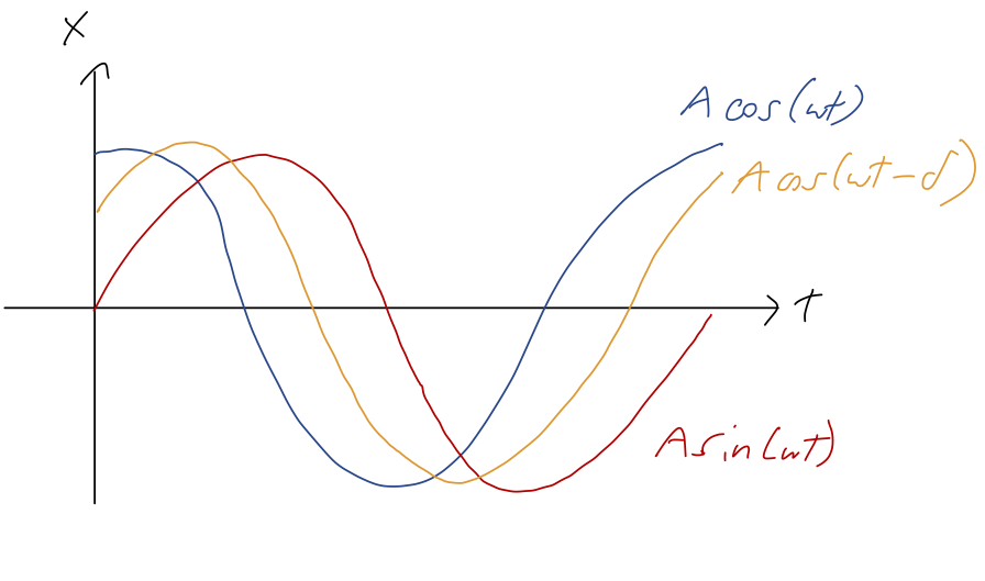
Instead of trying to find A directly, we’ll just rewrite our general solution in a different form. We know that trig identities let us combine sums of sine and cosine into a single trig function. Thus, the general solution must also be writable in the form x(t) = A \cos (\omega t - \delta) where now A and \delta are the arbitrary constants. In this form, it’s easy to see that A is exactly the amplitude, since the maximum of a single trig function is at \pm 1. We could relate A and \delta back to B_1 and B_2 using trig identities (look in Taylor), but instead we can just re-apply the initial conditions to this form: x_0 = x(0) = A \cos (-\delta) = A \cos \delta \\ v_0 = \dot{x}(0) = -\omega A \sin(-\delta) = \omega A \sin \delta
using trig identities to simplify. (We used -\delta instead of +\delta inside our general solution to ensure that there are no minus signs in these equations, in fact.) To compare a little more closely between forms, we see that if we start from rest and at positive x_0, we must have \delta = 0 and so x(t) = A \cos (\omega t) = x_0 \cos (\omega t). On the other hand, if we start at x=0 but with a positive initial speed v_0, we must have \delta = \pi/2 to match on, and so x(t) = A \cos \left(\omega t - \frac{\pi}{2}\right) = A \sin (\omega t) = \frac{v_0}{\omega} \sin (\omega t). In between the pure-cosine and pure-sine cases, for \delta between 0 and \pi/2, we have that both position and speed are non-zero at t=0. We can visualize the resulting motion as simply a phase-shifted version of the simple cases, with the phase shift \delta determining the offset between the initial time and the time where x=A:
Earlier, we found that the amplitude is related to the total energy as E = \frac{1}{2} kA^2. We can verify this against our solutions with an A in them: if we start at x=A from rest, then E = U_0 = \frac{1}{2} kx(0)^2 = \frac{1}{2} k A^2 and if we start at x=0 (so U=0) at speed v_0, then E = T_0 = \frac{1}{2} mv_0^2 = \frac{1}{2} kA^2 \\ A = \sqrt{\frac{m}{k}} v_0 = \frac{v_0}{\omega} which matches what we found above comparing our two solution forms. In fact, it’s easy to show using the phase-shifted cosine solution that E = \frac{1}{2}kA^2 always - I won’t go through the derivation, but it’s in Taylor.
Here, you should complete Tutorial 5A on “Simple Harmonic Motion”. (Tutorials are not included with these lecture notes; if you’re in the class, you will find them on Canvas.)
We’re not quite done yet: there is actually yet another way to write the general solution, which will just look like a rearrangement for now but will be extremely useful when we add extra forces to the problem. But to understand it, we need to take a brief math detour into the complex numbers.
5.2 Complex numbers
This is one of those topics that I suspect many of you have seen before, but you might be rusty on the details. So I will go quickly over the basics; if you haven’t seen this recently, make sure to review it elsewhere as well (the optional/recommended book by Boas is a good resource.)
Complex numbers are an important and useful extension of the real numbers. In particular, they can be thought of as an extension which allows us to take the square root of a negative number. We define the imaginary unit as the number which squares to -1, i^2 = -1. (Note that some books - mostly in engineering, particularly electrical engineering - will call the imaginary unit j instead, presumably because they want to reserve i for electric current.) This definition allows us to identify the square root of a negative number by including i, for example the combination 8i will square to (8i)^2 = (64) (-1) = -64 so \sqrt{-64} = 8i.
Actually, we should be careful: notice that -8i also squares to -64. Just as with the real numbers, there are two square roots for every number: +8i is the principal root of -64, the one with the positive sign that we take by default as a convention.
This ambiguity extends to i itself: some books will start with the definition \sqrt{-1} = i, but we could also have taken -i as the square root of -1 and everything would work the same. Defining i using square roots is also dangerous, because it leads you to things like this “proof”: 1 = \sqrt{1} = \sqrt{(-1) (-1)} = \sqrt{-1} \sqrt{-1} = i^2 = -1?? This is obviously wrong, because it uses a familiar property of square root that isn’t true for complex numbers: \sqrt{ab} \neq \sqrt{a} \sqrt{b} no longer works if any negatives are involved under the roots.
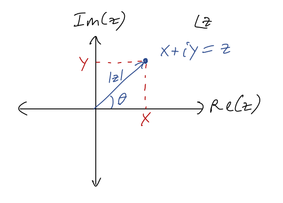
Since we’ve only added the special object i, the most general possible complex number is z = x + iy where x and y are both real. This observation leads to the fact that the complex numbers can be thought of as two copies of the real numbers. In fact, we can use this to graph complex numbers in the complex plane: if we define {\textrm{Re}}(z) = x \\ {\textrm{Im}}(z) = y as the real part and imaginary part of z, then we can draw any z as a point in a plane with coordinates (x,y) = ({\textrm{Re}}(z), {\textrm{Im}}(z)):
Obviously, numbers along the real axis here are real numbers; numbers on the vertical axis are called imaginary numbers or pure imaginary.
In complete analogy to polar coordinates, we define the magnitude or modulus of z to be |z| = \sqrt{x^2 + y^2} = \sqrt{{\textrm{Re}}(z)^2 + {\textrm{Im}}(z)^2}. We can also define an angle \theta, as pictured above, by taking \theta = \tan^{-1}(y/x) (being careful about quadrants.) This is very useful in a specific context - we’ll come back to it in a moment.
First, one more definition: for every z = x + iy, we define the complex conjugate z^\star to be z^\star = x - iy (More notation: in math books this is sometimes written \bar{z} instead of z^\star; physicists tend to prefer the star notation.) In terms of the complex plane, this is a mirror reflection across the x-axis. We note that zz^\star = (x+iy)(x-iy) = x^2 - i^2 y^2 = x^2 + y^2 so zz^\star = |z|^2 = |z^\star|^2 (the last one is true since (z^\star)^\star = z.)
Using the complex conjugate, we can write down explicit formulas for the real and imaginary parts: {\textrm{Re}} (z) = \frac{1}{2} (z + z^\star) \\ {\textrm{Im}} (z) = \frac{1}{2i} (z - z^\star). You can plug in z = x + iy and easily verify these formulas give you x and y respectively.
Multiplying and dividing complex numbers is best accomplished by doing algebra and using the definition of i. For example, (2+3i)(1-i) = 2 - 2i + 3i - 3i^2 \\ = 5 + i Division proceeds similarly, except that we should always use the complex conjugate to make the denominator real. For example, \frac{2+i}{3-i} = \frac{2+i}{3-i} \frac{3+i}{3+i} \\ = \frac{6 + 5i + i^2}{9 - i^2} \\ = \frac{6 + 5i - 1}{9 + 1} \\ = \frac{5+5i}{10} = \frac{1}{2} + \frac{i}{2}. The most important division rule to keep in mind is that dividing by i just gives an extra minus sign, e.g. \frac{2}{i} = \frac{2i}{i^2} = -2i.
Now, finally to the real reason we’re introducing complex numbers: an extremely useful equation called Euler’s formula. To find the formula, we start with the series expansion of the exponential function: e^x = 1 + x + \frac{x^2}{2!} + \frac{x^3}{3!} + \frac{x^4}{4!} + ... Series expansions are just as valid over the complex numbers as over the real numbers (with some caveats, but definitely and always true for the exponential.) What happens if we plug in an imaginary number instead of a real one? Let’s try x = i\theta, where \theta is real: e^{i\theta} = 1 + i\theta + \frac{(i\theta)^2}{2!} + \frac{(i\theta)^3}{3!} + \frac{(i\theta)^4}{4!} + ... Multiplying out all the factors of i and rearranging, we find this splits into two series, one with an i left over and one which is completely real: e^{i\theta} = \left(1 - \frac{\theta^2}{2!} + \frac{\theta^4}{4!} + ... \right) + i \left( \theta - \frac{\theta^3}{3!} + ... \right) Those other two series should look familiar: they are exactly the Taylor series for the trig functions \cos \theta and \sin \theta! Thus, we have:
For a real number \theta,
e^{i\theta} = \cos \theta + i \sin \theta.
This is an extremely useful and powerful formula, that makes complex numbers much easier to work with! Notice first that |e^{i\theta}| = \cos^2 \theta + \sin^2 \theta = 1. So e^{i\theta} is always on the unit circle - and as the notation suggests, the angle \theta is exactly the angle in the complex plane of this number. This leads to the polar notation for an arbitrary complex number, z = x + iy = |z| e^{i\theta}. The polar version is much easier to work with for multiplying and dividing complex numbers: z_1 z_2 = |z_1| |z_2| e^{i(\theta_1 + \theta_2)} \\ z_1 / z_2 = |z_1| / |z_2| e^{i(\theta_1 - \theta_2)} \\ z^\alpha = |z|^\alpha e^{i\alpha \theta} For that last one, we see that taking roots is especially nice in polar coordinates. For example, since i = e^{i\pi/2}, we have \sqrt{i} = (e^{i\pi/2})^{1/2} = e^{i\pi/4} = \frac{1}{\sqrt{2}} (1+i) which you can easily verify. (This is the principal root, actually; the other possible solution is at e^{5i \pi/4}, which is -1 times the number above.)
Here, you should complete Tutorial 5B on “Complex Numbers”. (Tutorials are not included with these lecture notes; if you’re in the class, you will find them on Canvas.)
Express the complex number \frac{1}{1-i} in polar notation |z|e^{i\theta}.
Answer:
There are two ways to solve this problem. We’ll start with Euler’s formula, which I promised would make things easier! Using 1-i = |z| (\cos(\theta) + i \sin (\theta)) we first see that we’re looking for an angle where \cos and \sin are equal in magnitude (which means \pi/4, 3\pi/4, 5\pi/4, or 7\pi/4.) Since \cos is positive while \sin is negative, this points us to quadrant IV, so \theta = 7\pi/4 - I’ll use \theta = -\pi/4 equivalently. Meanwhile, the complex magnitude is |z| = \sqrt{1^2 + (-1)^2} = \sqrt{2} so we have 1-i = \sqrt{2} e^{-i\pi/4}. If you prefer to just plug in to formulas, we can also get this with \tan^{-1}(y/x) = \theta, but we still have to be careful about quadrants. In fact, an even simpler way to find this result would probably have been to just draw a sketch in the complex plane.
Inverting this is easy: we get \frac{1}{1-i} = \frac{1}{\sqrt{2}} e^{i\pi/4} = \frac{1}{2} (1+i). You can easily verify from the second form here that multiplying this by (1-i) gives 1.
The second way to solve this problem without polar angles is to multiply through the numerator and denominator by the complex conjugate: \frac{1}{1-i} = \frac{1+i}{(1-i)(1+i)} This gives us a difference of squares in the denominator which will get rid of the imaginary part: \frac{1+i}{(1-i)(1+i)} = \frac{1+i}{1^2 - i^2} = \frac{1}{2} (1+i) This matches what we got above; we can also convert back to polar form with 1+i = \sqrt{2} e^{i\pi/4} recovering the answer in polar as well.
Back to Euler’s formula itself: we can invert the formula to find useful equations for \cos and \sin. I’ll leave it as an exercise to prove the following identities: \cos \theta = \frac{1}{2} (e^{i\theta} + e^{-i\theta}) \\ \sin \theta = \frac{-i}{2} (e^{i\theta} - e^{-i\theta}) (These are, incidentally, extremely useful in simplifying integrals that contain products of trig functions. We’ll see this in action later on!)
5.2.1 Complex solutions to the SHO
Back to the SHO equation, \ddot{x} = -\omega^2 x The minus sign in the equation is very important. We saw before that for equilibrium points that are unstable, the equation of motion we found near the equilibrium was \ddot{x} = +\omega^2 x. This equation has solutions that are exponential in t, moving rapidly away from equilibrium.
But now that we’ve introduced complex numbers, we can also write an exponential solution to the SHO equation. Notice that if we take x(t) = e^{i\omega t}, then \ddot{x} = \frac{d}{dt} (i \omega e^{i \omega t}) = (i \omega)^2 e^{i \omega t} = -\omega^2 e^{i\omega t} and so this satisfies the equation. So does the function e^{-i\omega t} - the extra minus sign cancels when we take two derivatives. These are independent functions, even though they look very similar; there is no constant we can multiply e^{i\omega t} by to get e^{-i \omega t}. Thus, another way to write the general solution is x(t) = \frac{C_1}{2} e^{i\omega t} + \frac{C_2}{2} e^{-i \omega t}. (The division by 1/2 is arbitrary since we don’t know the constants yet, but it will cancel off another 2 later to make our answer nicer.)
Now, this is a physics class (and we’re not doing quantum mechanics!), so obviously the position of our oscillator x(t) always has to be a real number. However, by introducing i we have found a solution for x(t) valid over the complex numbers. The only way that this can make sense is if choosing physical (i.e. real) initial conditions for x(0) and \dot{x}(0) gives us an answer that stays real for all time; otherwise, we’ve made a mistake somewhere.
Let’s see how this works by imposing those initial conditions: we have x(0) = x_0 = \frac{1}{2} (C_1 + C_2) \\ v(0) = v_0 = \frac{i\omega}{2} (C_1 - C_2) This obviously only makes sense if C_1 + C_2 is real and C_1 - C_2 is pure imaginary - which means the coefficients C_1 and C_2 have to be complex! (This isn’t a surprise, since we asked for a solution over complex numbers.) If we write C_1 = x + iy then the conditions above mean that we must have C_2 = x - iy so the real and imaginary parts cancel appropriately. In other words, we must have a general solution of the form x(t) = C_1 e^{i\omega t} + C_1^\star e^{-i\omega t}. This might look confusing, since we now seemingly have one arbitrary constant instead of the two we need. But it’s one arbitrary complex number, which is equivalent to two arbitrary reals. In fact, we can finish plugging in our initial conditions to find C_1 = x_0 - \frac{iv_0}{\omega} so both of our initial conditions are indeed separately contained in the single constant C_1.
Now, if we look at the latest form for x(t), we notice that the second term is exactly just the complex conjugate of the first term. Recalling the definition of the real part as {\textrm{Re}}(z) = \frac{1}{2} (z + z^\star), we can rewrite this more compactly as x(t) = {\textrm{Re}}\ (C_1 e^{i\omega t}). This is nice, because now x(t) is manifestly always real! (But remember that we did not just arbitrarily “take the real part” to enforce this; it came out of our initial conditions. It’s not correct to solve over the complex numbers and then just ignore half the solution!)
Here, you should complete Tutorial 5C on “Complex Solutions to the SHO”. (Tutorials are not included with these lecture notes; if you’re in the class, you will find them on Canvas.)
At this point, let’s try to compare back to our trig-function solutions; we know they’re hiding in there somehow, thanks to Euler’s formula.
Let’s verify that the real part written above gives back the previous general solution. The best way to do this is to expand our all the complex numbers into real and imaginary components, do some algebra, and then just read off what the real part of the product is. Let’s substitute in using both C_1 from above and Euler’s formula: x(t) = {\textrm{Re}}\ \left[ \left( x_0 - \frac{iv_0}{\omega} \right) \left( \cos (\omega t) + i \sin (\omega t) \right) \right] Multiplying through, x(t) = {\textrm{Re}}\ \left[ x_0 \cos(\omega t) + ix_0 \sin (\omega t) - \frac{iv_0}{\omega} \cos (\omega t) + \frac{v_0}{\omega} \sin (\omega t) \right] \\ = {\textrm{Re}}\ \left[ x_0 \cos (\omega t) + \frac{v_0}{\omega} \sin (\omega t) + i (...) \right] \\ = x_0 \cos (\omega t) + \frac{v_0}{\omega} \sin (\omega t) just ignoring the imaginary part. So indeed, this is exactly the same as our previous solution, just in a different form!
This is a nice confirmation, but the fact that C_1 is complex makes it a little non-obvious what the real and imaginary parts look like. We can fix that by rewriting it in polar notation. If I suggestively define C_1 = A e^{-i\delta}, then we have x(t) = {\textrm{Re}}\ (A e^{-i\delta} e^{i\omega t}) = A\ {\textrm{Re}}\ (e^{i(\omega t - \delta)}) pulling the real number A out of the real part. Now taking the real part of the combined complex exponential is easy: it’s just the cosine of the argument, x(t) = A \cos (\omega t - \delta), exactly matching the other form of the SHO solution we wrote down before. (Notice: no need for trig identities this time! Complex exponentials are a very powerful tool for simplfying expressions involving trig functions.)
One last thing to point out: although nothing I’ve written so far is incorrect, we should be a little bit careful when we want to write the velocity v_x(t) directly using the complex solution. We have: v_x(t) = \frac{dx}{dt} = \frac{d}{dt} {\textrm{Re}} (C_1 e^{i\omega t})
We can’t just push the derivative through the real part, or we’ll get the wrong answer! To find what the derivative does, we should expand out using the definition of Re: v_x(t) = \frac{d}{dt} \frac{1}{2} \left( C_1 e^{i\omega t} + C_1^\star e^{-i\omega t} \right) \\ = \frac{1}{2} C_1 i \omega e^{i\omega t} - \frac{1}{2} C_1^\star i \omega e^{-i\omega t} \\ = \frac{i \omega}{2} \left( C_1 e^{i\omega t} - C_1^\star e^{-i\omega t} \right) \\ = -\omega {\textrm{Im}} (C_1 e^{i\omega t}).
I’m going to more or less skip over the two-dimensional oscillator; as we emphasized before, one-dimensional motion is special in terms of what we can learn from considering energy conservation, and similarly the SHO is especially useful in one dimension. Of course, the idea of expanding around equilibrium points is very general, but it will not just give you the 2d or 3d SHO equation that Taylor studies in (5.3). In general, you will end up with a coupled harmonic oscillator, the subject of chapter 11.
We can see a little bit of why the 2d SHO is a narrow special case by just considering the seemingly simple example of a mass on a spring connected to the origin in two dimensions. If the equilibrium (unstretched) length of the spring is r_0, then \vec{F} = -k(r- r_0) \hat{r} or expanding in our two coordinates, using r = \sqrt{x^2 + y^2} and \hat{r} = \frac{1}{r} (x\hat{x} + y\hat{y}), m \ddot{x} = -kx (1 - \frac{r_0}{\sqrt{x^2 + y^2}}) \\ m \ddot{y} = -ky (1 - \frac{r_0}{\sqrt{x^2 + y^2}}) These equations of motion are much more complicated than the regular SHO, and in particular we see they are coupled: both x and y appear in both equations. The regular two-dimensional SHO appears when r_0 = 0, and we just get two nice uncoupled SHO equations; but as I said, this is a special case, so I’ll just let you read about it in Taylor.
Our complex solutions have already proved useful, but they will be even more helpful as we move beyond the simple harmonic oscillator to more interesting and complicated variations next.
5.3 The damped harmonic oscillator
For expanding around equilibrium, the SHO is all we need, and we’ve solved it thoroughly at this point. However, it turns out there’s a lot of interesting physics and math in variations of the harmonic oscillator that have nothing to do with equilibrium expansion or energy conservation.
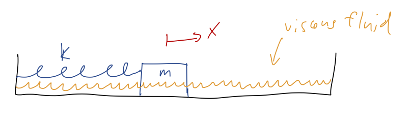
We’ll begin our study with the damped harmonic oscillator. Damping refers to energy loss, so the physical context of this example is a spring with some additional non-conservative force acting. Specifically, what people usually call “the damped harmonic oscillator” has a force which is linear in the speed, giving rise to the equation m \ddot{x} = - b\dot{x} - kx. The new force is the familiar linear drag force, so we can imagine this to be the equation describing a mass on a spring which is sliding through a high-viscosity fluid, like molasses:
As Taylor observes, another very important instance of this equation is the LRC circuit, which contains an inductor, a resistor, and a capacitor in series. The differential equation for the charge in such a circuit is L\ddot{Q} + R\dot{Q} + \frac{Q}{C} = 0. Since this is not a circuits class I won’t dwell on this example, but I point it out for those of you who might be more familiar with circuit equations.
Let’s rearrange the equation of motion slightly and divide out by the mass, as we did for the SHO: \ddot{x} + 2\beta \dot{x} + \omega_0^2 x = 0 where \beta = \frac{b}{2m},\ \ \omega_0 = \sqrt{\frac{k}{m}}, using the conventional notation for this problem. The frequency \omega_0 is called the natural frequency; as we can see, it is the frequency at which the system would oscillate if we removed the damping term by setting b=0. The other constant \beta is called the damping constant, and it is proportional to the strength of the drag force. \beta has the same units as \omega_0, i.e. frequency or 1/time.
5.3.1 Solving 2nd-order linear ODEs using operators
Once again, we have a linear, second-order, homogeneous ODE, so we just need to find two independent solutions to put together. Unfortunately, it’s a little harder to guess what the solutions will be just by inspection this time. Taylor uses the first method most physicists will reach for - guess and check, here guessing a complex exponential form. This sort of works, but in the special case \beta = \omega_0 (which we do want to cover) guess and check is much harder to use.
There is a more systematic way to find the answer, using the language of linear operators (as covered in Boas 8.5.) First of all, an operator is a generalized version of a function: it’s a map that takes an input to an output based on some specific rules. The derivative d/dt can be thought of as an operator, which takes an input function and gives us back an output function. The “linear” part refers to operators that follow two simple rules:
\frac{d}{dt} (f(t) + g(t)) = \frac{df}{dt} + \frac{dg}{dt}
\frac{d}{dt} (a f(t)) = a \frac{df}{dt}
We already know that these are both true for d/dt. What this means is that we can do algebra on the derivative operator itself. For example, using these properties we can write \frac{d^2f}{dt^2} + 3\frac{df}{dt} = 0 \Rightarrow \frac{d}{dt} \left( \frac{d}{dt} + 3 \right) f(t) = 0 or adopting the useful shorthand that D \equiv d/dt, D (D+3) f(t) = 0 = (D+3) D f(t).
On the last line, I re-ordered the two derivative terms. But this reordering is very useful, because it shows that there are two ways to satisfy the equation: both D f(t) = 0 and (D+3) f(t) = 0 will lead to solutions to the differential equation. Even better, the two solutions we get will be linearly independent (I won’t prove this, see Boas), which means that solving each of these simple first-order equations immediately gives us the general solution to the original equation!
This gives us a very useful method to solve a whole class of second-order linear ODEs:
Rewrite the ODE in the form (aD^2 + bD + c) f = 0.
Solve for the roots of the auxiliary equation, (aD^2 + bD + c) = 0 = (D - r_1) (D - r_2)
Obtain the general solution from the solutions of (D-r_1) f = 0 and (D - r_2) f = 0.
Here I’ve assumed a homogeneous ODE, i.e. the right-hand side is zero. We can use the same method for non-homogeneous equations, but there’s an extra step in that case: we have to add a particular solution, as we saw in the first-order case. Also, it’s very important above that the constants are constant - in other words, if D = d/dt, then a,b,c must all be independent of t or else the reordering trick doesn’t work (it’s easy to see that, for example, D (D+t) is not equal to (D+t) D.)
Now let’s use this method on the damped harmonic oscillator. Our ODE looks like \ddot{x} + 2\beta \dot{x} + \omega_0^2 x = 0 which we can rewrite as (D^2 + 2\beta D + \omega_0^2) x(t) = 0. To find the roots of the auxiliary equation, we can just use the quadratic formula: r_{\pm} = -\beta \pm \sqrt{\beta^2 - \omega_0^2}. The individual solutions, then, solve the first-order equations (D - r_{\pm}) x = 0, which we recognize as simple exponential solutions, x(t) \propto e^{r_{\pm} t}.
Thus, our general solution is: x(t) = C_1 e^{r_+ t} + C_2 e^{r_- t} \\ = C_1 e^{-\beta t + \sqrt{\beta^2 - \omega_0^2} t} + C_2 e^{-\beta t - \sqrt{\beta^2 - \omega_0^2} t} \\ = e^{-\beta t} \left( C_1 e^{\sqrt{\beta^2 - \omega_0^2} t} + C_2 e^{-\sqrt{\beta^2 - \omega_0^2}t} \right). (There is one subtlety here: if r_+ = r_-, then we have actually only found one solution. I’ll return to this case a little later.)
If we plug in \beta = 0 as a check, then we get \sqrt{-\omega_0^2} t = i\omega_0 t inside both of the exponentials in the second factor, giving back our undamped SHO solution as it should.
It should be obvious from looking at this that the relative size of \beta and \omega_0 will be very important in the qualitative behavior of these solutions: the exponentials inside the parentheses can be either real or imaginary as we change \beta relative to \omega_0. Let’s go through the possibilities.
5.3.2 Underdamped motion
Since we already know what happens at \beta = 0, let’s start with small \beta and turn the strength of the force up from there. (\beta is dimensionless, so by “small \beta” I of course mean “small \beta/\omega_0.”) In particular, as long as \beta < \omega_0, the combination \beta^2 - \omega_0^2 under the roots will always be negative. We define a new frequency \omega as follows: \sqrt{\beta^2 - \omega_0^2} = i \sqrt{\omega_0^2 - \beta^2} = i \omega_1. Why \omega_1? I am not sure, other than 1 is the number after 0! But I’ll stick with this notation because it’s what Taylor uses, and because we have to call this something other than \omega_0 (which we are already using) and \omega (which we will need for something else shortly.)
With this definition, we have for the overall solution x(t) = e^{-\beta t} \left(C_1 e^{i\omega_1 t} + C_2 e^{-i\omega_1 t} \right), or doing the same trick to combine the trig functions as before, x(t) = Ae^{-\beta t} \cos (\omega_1 t - \delta). So we once again have an oscillating solution, almost the same as the SHO, except the amplitude dies off exponentially as e^{-\beta t}. If we plot this, we can imagine an exponential “envelope” given by \pm Ae^{-\beta t}, with the actual solution oscillating back and forth between the sides of the envelope:
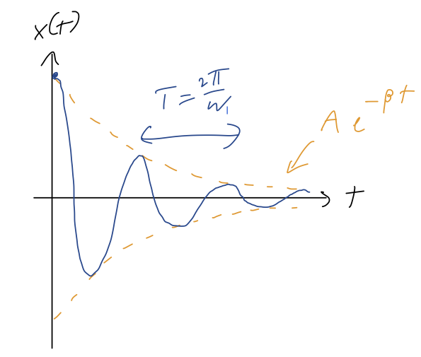
The solution above corresponds to releasing the oscillator at rest from some initial displacement. Note that this is no longer periodic, but the distance between maxima or minima within the envelope is still \tau = 2\pi / \omega_1. If \beta \ll \omega_0, then we notice that \omega_1 \approx \omega_0, so for very small damping the oscillation frequency is roughly the same as the natural oscillation. As the damping increases, the frequency of oscillation decreases (the peaks get further apart.)
By the way, notice what happens if we impose initial conditions on our simple harmonic oscillator solution: x(0) = A \cos(-\delta) \\ \dot{x}(0) = -A (\beta \cos (-\delta) + \omega_1 \sin(-\delta)) We can see right away that this is going to be trickier than the regular SHO solution; in particular, it is not true that \delta = 0 gives us the solution starting from rest here! Using some trig identities, this leads to the set of equations x(0) = A \cos \delta \\ \dot{x}(0) = -A \beta \cos \delta \left[1 - \frac{\omega_1}{\beta} \tan \delta \right]. This gets messy to solve, but for the specific case of starting from rest, \dot{x}(0) = 0 leads us to the simpler result 1 - \frac{\omega_1}{\beta} \tan \delta = 0 \Rightarrow \delta = \tan^{-1} \left( \frac{\omega_1}{\beta} \right) = \tan^{-1} \left( \frac{\sqrt{\omega_0^2 - \beta^2}}{\beta} \right) which we can plug in to for the phase shift, and then plug in to the first equation to find A. I won’t go further with this - you’d want to do it numerically for a given oscillator, the general case isn’t very enlightening. But I wanted to point out that A and \delta don’t have quite the same simple interpretations anymore for the damped oscillator.
5.3.3 Overdamped motion
Let’s move on to the case where \beta > \omega_0 - exact equality is tricky, so we’ll do that last. In this case, all of the exponentials stay real, and we have x(t) = C_1 e^{-(\beta - \sqrt{\beta^2 - \omega_0^2}) t} + C_2 e^{-(\beta + \sqrt{\beta^2 - \omega_0^2}) t}. Since \sqrt{\beta^2 - \omega_0^2} < \beta given our assumptions, both terms decay exponentially in time, and there’s no oscillation at all. Here’s a sketch of this solution:
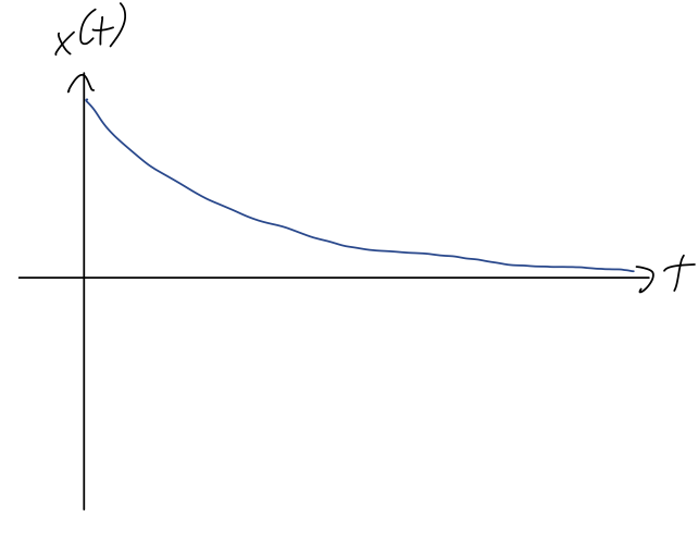
It’s instructive to factor out the first exponential term completely from our solution: x(t) = e^{-(\beta - \sqrt{\beta^2 - \omega_0^2}) t} \left( C_1 + C_2 e^{-2\sqrt{\beta^2 - \omega_0^2} t}\right). As t increases, the second term here is negligible for the long-term behavior of the system, unless we have C_1 = 0. Let’s match initial conditions to see what that would require: x_0 = x(0) = C_1 + C_2 \\ v_0 = \dot{x}(0) = -(\beta - \sqrt{\beta^2 - \omega_0^2}) C_1 - (\beta + \sqrt{\beta^2 - \omega_0^2}) C_2 We can solve this for C_1 = 0, and a bit of algebra reveals that it requires a specific relationship between v_0 and x_0, \frac{v_0}{x_0} = -(\beta + \sqrt{\beta^2 - \omega_0^2}). In particular, the minus sign tells us that this is only possible if v_0 and x_0 are in opposite directions. Aside from this rather special case, we can in general ignore the C_2 term completely at large t, finding that x(t) \rightarrow C_1 e^{-\alpha t} defining the decay parameter \alpha as the coefficient in the exponential decay of the max amplitude at large t, in this case \alpha = \beta - \sqrt{\beta^2 - \omega_0^2}. This solution exhibits some rather counterintuitive behavior: as we increase the strength of the damping force \beta, the decay parameter \alpha actually becomes smaller, approaching \alpha = 0 as \beta \rightarrow \infty! To make sense of this, let’s remember that the net force on our oscillator is F_{\textrm{net}} = F_{\textrm{drag}} + F_{\textrm{spring}} = -2m\beta \dot{x} - k x Both forces push our object back towards the origin. But if \beta is extremely large, then there is an enormous force even if we try to move at a relatively small speed, so it will take much longer in time for us to actually get to the origin. We still get there eventually, because the -kx spring force always keeps pulling us to the origin as long as x is non-zero.
5.3.4 Critical damping
Finally, we come back to the third possibility, which is \beta = \omega_0. If we go back to our original solution, this gives us x(t) = C_1 e^{-(\beta - \sqrt{\beta^2 - \omega_0^2}) t} + C_2 e^{-(\beta + \sqrt{\beta^2 - \omega_0^2}) t} \rightarrow C_1 e^{-\beta t} + C_2 e^{-\beta t}. Now we only have one solution, repeated twice! This means our solution is suddenly incomplete: we need two independent functions to add together to have a general solution. To find a second solution, since this is clearly a special case, let’s go back to the original differential equation and see what happens if \beta = \omega_0: \ddot{x} + 2 \beta \dot{x} + \beta^2 x = 0 Clearly e^{-\beta t} indeed works as a solution. To see the other one, let’s go back to our linear operator language and notice that the auxiliary equation in this case is easy to factorize: \left( \frac{d^2}{dt^2} + 2\beta \frac{d}{dt} + \beta^2 \right) x(t) = 0 becomes \left( D + \beta \right) \left( D + \beta \right) x(t) = 0. One way that this equation can be satisfied is just if \left( D + \beta \right) x(t) = 0, which matches on to our solution e^{-\beta t}. But the other possibility is that this combination isn’t zero: let’s call it \left( D + \beta \right) x(t) = u(t) \neq 0. Then we’re left with another first-order ODE, \left( D + \beta \right) u(t) = 0. So u(t) = C e^{-\beta t}, but now we have to work backwards a bit: \left( D + \beta \right) x(t) = C e^{-\beta t} We can use the general first-order solution in Boas to find the answer directly, but if you stare at this for a minute, you might think to try the following combination: if x(t) = C t e^{-\beta t} then \frac{dx}{dt} = C e^{-\beta t} - \beta C t e^{-\beta t} so the te^{-\beta t} will cancel out, matching the right-hand side. Thus, the general solution in this special case where \beta = \omega_0 is x(t) = C_1 e^{-\beta t} + C_2 t e^{-\beta t}. Once again, we see no oscillations - everything is pure exponential decay, but with an extra factor of t that only matters at small times. Once again as t becomes very large, the amplitude decays exponentially proportional to \beta.
5.3.5 Damped oscillator summary
Let’s summarize all of our solutions:
If \beta < \omega_0, the system is said to be underdamped. Our solution takes the form x(t) = Ae^{-\beta t} \cos (\omega_1 t - \delta), with oscillations at angular frequency \omega_1 = \sqrt{\omega_0^2 - \beta^2}, and the overall amplitude decaying with decay parameter \alpha = \beta.
If \beta = \omega_0, the system is critically damped. We have the funny solution we just found, x(t) = C_1 e^{-\beta t} + C_2 t e^{-\beta t}, with no oscillations and again the ampltiude at large times decaying exponentially with \alpha = \beta.
Finally, if \beta > \omega_0, the system is overdamped. In this case the general solution looks like x(t) = C_1 e^{-(\beta - \sqrt{\beta^2 - \omega_0^2}) t} + C_2 e^{-(\beta + \sqrt{\beta^2 - \omega_0^2}) t}. again pure exponential decay, but this time with decay parameter \alpha = \beta - \sqrt{\beta^2 - \omega_0^2}, which goes to zero as \beta gets larger and larger.
We can sketch the size of the decay parameter vs. the damping parameter \beta:
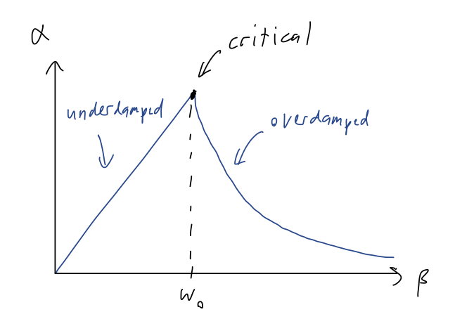
When designing a system that behaves like a damped oscillator, this tells us that it’s actually optimal to tune \beta (or \omega_0) so that the system is as close to critical as possible. A good example is shock absorbers in a car, which are designed to damp out the oscillations transferred from the road to the passengers.
5.3.6 Visualization using phase space
Let’s jump back for a moment to the simple harmonic oscillator (\beta = 0.) Given any solution for the position x(t), we also know the speed \dot{x}(t) of our oscillator at any given time. For example, using the phase-shift version of the solution: x(t) = A \cos (\omega t - \delta) \\ \Rightarrow \dot{x}(t) = -\omega A \sin (\omega t - \delta). Since we have a sine and a cosine, this is strongly reminiscent of polar coordinates with \phi = \omega t. In fact, we can make a nice plot by picking “coordinates” with \omega x on one axis and \dot{x} on the other:
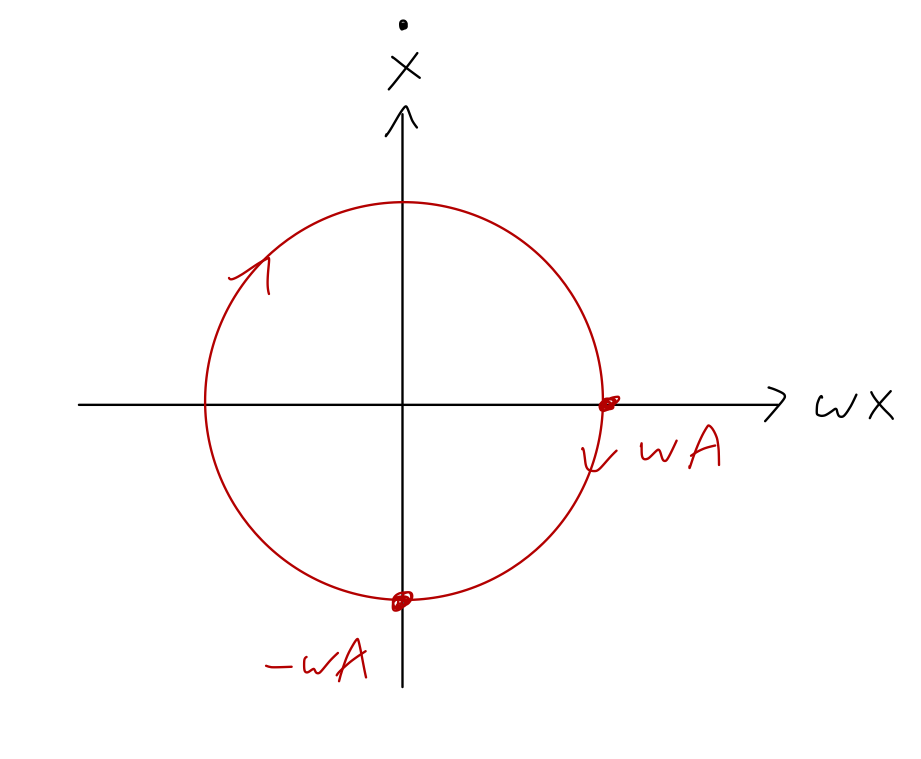
This fictitious space, mixing position and speed with each other, is known as phase space. (Some references will just use x and \dot{x} as the axes, instead of \omega x and \dot{x}; since this is a fictitious space that we made up, the dimensions don’t have to match. But I’m going to keep the version with the \omega since it will simplify things a bit below.)
If we take a snapshot of our harmonic oscillator at any given moment t, recording x and \dot{x}, we obtain a single point in phase space. Letting t evolve for a given system then traces out a curve known as a phase portrait. Phase portraits are a useful way to visualize the behavior of a physical system.
Here, you should complete Tutorial 5D on “Phase space and harmonic motion”. (Tutorials are not included with these lecture notes; if you’re in the class, you will find them on Canvas.)
It’s useful to recall that the total energy of our harmonic oscillator is E = \frac{1}{2} m\dot{x}^2 + \frac{1}{2} kx^2 \\ = \frac{m}{2} \left( \dot{x}^2 + \omega^2 x^2 \right) using \omega^2 = k/m. This is just the equation of a circle in phase space the way we have defined the axes, with radius \sqrt{2E/m}. So another way to derive the “circular” motion in phase space is just that total energy E is constant for the simple harmonic oscillator!
As a comment: although I am starting with \omega x on the horizontal axis, this choice does have some drawbacks. For example, we can’t compare the phase portraits of two different oscillators easily, because we can only rescale by one frequency \omega. For more general applications of phase space, it is often better to just keep the axes as x vs. \dot{x}, in which case the energy conservation equation is written in the same way but interpreted slightly differently: 1 = \frac{x^2}{(2E/k)} + \frac{\dot{x}^2}{(2E/m)}. This is the equation of an ellipse, (x/a)^2 + (y/b)^2 = 1; the lengths of the semi-major axes are a=\sqrt{2E/k} and b=\sqrt{2E/m} = \omega \sqrt{2E/k} = \omega a.
Let’s continue on to the damped case. Since the phase-space orbit of the SHO is a circle (or ellipse, more generally) due to energy conservation, we expect that damping will drive our system towards the origin of phase space, (x, \dot{x}) = (0,0), as energy is removed and it comes to a stop. Starting with the underdamped case and taking a derivative, the speed is \dot{x}(t) = -\beta A e^{-\beta t} \cos (\omega_1 t - \delta) - \omega_1 A e^{-\beta t} \sin (\omega_1 t - \delta) or making the variable definition \phi = \omega_1 t - \delta, x(t) = Ae^{-\beta t} \cos \phi \\ \dot{x}(t) = -Ae^{-\beta t} (\beta \cos \phi + \omega_1 \sin \phi) This is already in a form that we can plug in to Mathematica to make a parametric plot using \phi, in order to visualize the phase-space trajectory (remember to substitute out t = (\phi + \delta) / \omega_1.) To go a little further by hand, let’s consider the case of small damping, \beta \ll \omega_0 (and thus \omega_1 \approx \omega_0). Then we can neglect the \cos \phi term in the speed, and we have simply: \omega_0 x(t) = \omega_0 Ae^{-\beta t} \cos \phi \\ \dot{x}(t) = -\omega_0 Ae^{\beta t} \sin \phi This is just the parametric equation for a circle, x = \rho \cos \phi and y = -\rho \sin \phi, except that the radius is decreasing exponentially as e^{-\beta t} instead of constant! So the phase portrait in this case, sketching \omega_0 x vs. \dot{x}, will look like a spiral:
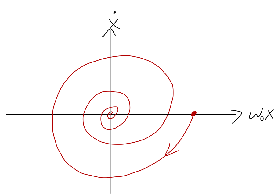
Increasing the damping \beta will distort the spiral a bit as the term we neglected becomes important, but the qualitative motion is still the same. This also makes sense with conservation of energy; we recall that the distance to the origin in phase space is equal to the total energy of the oscillator. That’s still true here - but with the damping term, the total energy is falling to zero as our system evolves in time.
We could also do phase-space visualizations for the overdamped and critically damped cases. However, like the plots of x(t) in those cases, they’re not very interesting visually; the system is just pushed from its initial conditions directly towards the origin. (In general, as we increase \beta the spiraling behavior in the underdamped case will get faster, and there will be less spirals around the origin. Moving into overdamping is just the limit in which there are no spirals left - the phase space path never makes a complete circuit around by 2\pi.)
5.4 The driven, damped SHO
There’s one more really important generalization we can add to the damped harmonic oscillator, which is a driving force. The damped oscillator is sort of a special case, because with no energy input the damping will quickly dispose of all the mechanical energy and cause the oscillator to stop. In many realistic applications (like a clock), we want an oscillator that will continue to oscillate, which means an external force has to be applied.
We’ll assume the applied force depends on time, but not on the position of the oscillator, so it takes the general form F(t). Then the ODE becomes m \ddot{x} + b \dot{x} + kx = F(t). (Again, if you’re familiar with circuits, this is like an LRC circuit adding in a source of electromotive force like a battery.)
With the addition of the driving force, our ODE is no longer homogeneous. This means that we no longer have the principle of superposition: we can’t find our general solution by just taking any two independent solutions and adding them together with constants.
Instead, we can use an old technique that we’ve seen for first-order equations. Suppose that we find a function x_c(t), the complementary solution, that just gives zero when plugged in to the left-hand side of the ODE, i.e. m \ddot{x}_c + b \dot{x}_c + kx_c = 0. (This equation with the non-homogeneous part thrown out is called the complementary equation.) Next, we find a function x_p(t) called the particular solution, which satisfies the full equation: m\ddot{x}_p + b\dot{x}_p + kx_p = F(t).
Although the particular solution works, since this is a linear second-order ODE, we know that the general solution requires two undetermined constants. We can’t add any constants to x_p itself; for example, 2x_p(t) is not a solution since it gives 2F(t) on the right-hand side. But since the complementary solution gives zero, we can add that in with an unknown constant.
Thus, the full general solution is x(t) = C_1 x_{1,c}(t) + C_2 x_{2,c}(t) + x_p(t) The good news is that we’ve already found the complementary solutions, since the complementary equation is just the regular damped oscillator that we just finished solving.
How we find the particular solution depends strongly on what the non-homogeneous part of the equation looks like. Constant is the simplest possibility: let’s do a quick example to demonstrate.
Let’s warm up by finding the general solution of the following equation:
\ddot{y} - \dot{y} - 6y = 4.
We start with the complementary equation, \ddot{y}_c - \dot{y}_c - 6y_c = 0
We can solve this using the algebra of differential operators: rewriting the complementary equation gives (D^2 - D - 6) y_c = 0 which we can factorize into (D+2)(D-3)y_c = 0. As usual we can write a simple exponential solution for each monomial: y_{1,c}(t) = e^{-2t},\ \ y_{2,c}(t) = e^{+3t}. On to the particular solution. We always want to look for a particular solution that has a similar form to the driving. A constant particular solution is especially nice, since all of the derivatives vanish immediately. It should be easy to see right away that y_p(t) = -\frac{2}{3} will satisfy the equation. Thus, putting everything together, we have for the general solution y(t) = C_1 e^{-2t} + C_2 e^{+3t} - \frac{2}{3}.
Coming back to the specific case of the oscillator, suppose that wehave a constant driving force F(t) = F_0. Rewriting the equation into our standard form, \ddot{x} + 2\beta \dot{x} + \omega_0^2 x = \frac{F_0}{m} so to our damped oscillator solutions from before, we simply have to add the particular solution x_p(t) = \frac{F_0}{m \omega_0^2}. This is just a constant offset to our x coordinate. So, for example, if we take an oscillator moving horizontally and reorient it so that it’s hanging vertically subject to gravity, the motion will be exactly the same except that the equilibrium position will be displaced to x_p = \frac{g}{\omega_0^2} = \frac{mg}{k} (which is exactly the new equilibrium point where the spring force kx_p balances the gravitational force mg.)
Let’s do a more interesting example of a driving force.
5.4.1 Complex exponential driving
Now we’ll assume a driving force of exponential form: F(t) = F e^{ct} where both F and c can be complex. This covers both regular exponential forces (if c is real), as well as the very important case of oscillating driving force (if c is imaginary.)
The obvious thing to try for our particular solution is exactly the same form: we’ll guess that x_p(t) = C_0 e^{ct} will give us a solution, and then try it out. Note that although I put in an unknown constant C_0, as we’ve seen with other particular solutions this is not an arbitrary constant; we expect only a specific choice of C_0 to work given a certain driving force.
Let’s plug our guessed solution back in and see what we get: from \ddot{x} + 2\beta \dot{x} + \omega_0^2 x = \frac{F}{m} e^{ct} we have \left[ c^2 + 2\beta c + \omega_0^2 \right] C_0 e^{ct} = \frac{F}{m} e^{ct} or cancelling off the exponentials, C_0 = \frac{F}{m(c^2 + 2\beta c + \omega_0^2)}. Once again, this is not arbitrary! Both c and F are given to us as part of the external driving force: they are literally numbers that are dialed in on whatever machine is providing the driving for our experiment.
Let’s step back for a moment and look at the big picture. Remember that the complementary solutions take the form e^{r_{\pm} t}, where r_{\pm} solve the equation r^2 + 2\beta r + \omega_0^2 = 0. The full solution is two complementary solutions with arbitrary coefficients, plus one particular: x(t) = C_+ e^{r_+ t} + C_- e^{r_- t} + C_0 e^{ct} with C_0 determined by F and c as we found above. All of these exponents can be complex, so we can have individual contributions that oscillate at one, two, or three different frequencies; we’ll make more sense of this soon.
Notice that there’s an important edge case here: the same quadratic equation for r appears again in the denominator of C_0. So if we have c = r_{\pm}, then our formula for C_0 blows up. This is similar to what happened in the critical damping case: our would-be particular solution fails, because it’s not independent from the complementary solution. The way to fix this, similarly, is to take a particular solution of the form C_0 te^{ct} or C_0 t^2 e^{ct} as needed (we only need the second one if the system is critically damped, so te^{ct} is already being used.)
5.4.2 Sinusoidal driving
So far this has been totally general, but real exponential driving forces are sort of an unusual special case; we won’t really be interested in them. So let’s specialize now to the very important case of an oscillating driving force, which we’ll write as follows: F(t) = F e^{ct} = F_0 e^{-i\delta_0} e^{i \omega t} so that c = i \omega, and we’ve split the complex force F into two real numbers F_0 and \delta_0. Plugging all of this back in to C_0 and splitting into real and imaginary parts in the denominator gives C_0 = \frac{F_0 e^{-i \delta_0}/m}{(\omega_0^2 - \omega^2) + 2i \beta \omega}. It will be useful to rewrite this in polar form, C_0 = Ae^{-i\Delta}. To find the amplitude A first, we multiply by the complex conjugate: |C_0|^2 = C_0 C_0^\star \\ = \frac{F_0e^{-i\delta_0}/m}{(\omega_0^2 - \omega^2) - 2i \beta \omega} \frac{F_0e^{+i \delta_0}/m}{(\omega_0^2 - \omega^2) + 2i \beta \omega} \\ = \frac{F_0^2/m^2}{(\omega_0^2 - \omega^2)^2 + 4\beta^2 \omega^2}, so the amplitude is A = |C_0| = \frac{F_0/m}{\sqrt{(\omega_0^2 - \omega^2)^2 + 4\beta^2 \omega^2}}. Next, the phase \Delta. We can simplify finding this by using the fact that the force is already in polar form, i.e. we can rewrite C_0 = Ae^{-i\Delta} = Ae^{-i(\delta_0 +\delta)} = Ae^{-i\delta_0} e^{-i\delta} defining the angle \delta to be the phase shift, i.e. the difference in phase between the input force phase \delta_0 and the particular solution phase \Delta. This lets us pull out the \delta_0 from C_0 like so: C_0 e^{+i\delta_0} = Ae^{-i\delta} \\ = \frac{F_0 /m}{(\omega_0^2 - \omega^2) + 2i \beta \omega} \left[\frac{(\omega_0^2 - \omega^2) - 2i \beta \omega}{(\omega_0^2 - \omega^2) - 2i \beta \omega}\right] \\ Ae^{-i\delta }= \frac{F_0/m}{(\omega_0^2 - \omega^2)^2 + 4\beta^2 \omega^2} \left[ (\omega_0^2 - \omega^2) - 2i \beta \omega \right]. where I’ve used the conjugate of the denominator to split this expression into real and imaginary parts.
Now, if we want to find \delta from this result, the factor in front of the square brackets doesn’t matter, since the angle only depends on the relative size of real and imaginary parts. The best way to see the answer is by making a quick sketch in the complex plane:
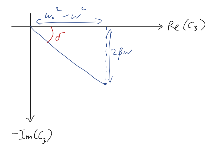
so we can read off that the complex phase is given by \tan \delta = \frac{2\beta \omega}{\omega_0^2 - \omega^2}. taking out a minus sign since we wrote this as Ae^{-i\delta} to begin with. (Or equivalently, the minus sign in Ae^{-i\delta} accounts for the fact that the imaginary part is negative, so the angle \delta in our sketch should be positive.) Incidentally, since \omega_0^2 - \omega^2 can have either sign but 2\beta \omega is always positive, we get a useful piece of information from our geometric picture: \delta can only be in quadrant 3 or 4 of the complex plane! In other words, with the conventional minus sign in Ae^{-i\delta}, we can only possibly have 0 < \delta < \pi. (The inequalities are strict because our solution only works with \beta > 0.)
Putting everything back together, our particular solution becomes x_p(t) = A e^{-i\Delta} e^{i\omega t}. with A = \frac{F_0/m}{\sqrt{\omega_0^2 - \omega^2)^2 + 4\beta^2 \omega^2}} and \tan \delta = \frac{2\beta \omega}{\omega_0^2 - \omega^2}
Once again, this has to be real since it’s a position. We’ve seen this before for the regular damped oscillator: once we are careful about plugging in initial conditions, the solution actually is real even though it looks complex. But this is the particular solution, so the initial conditions don’t affect it! So how do we make sure it’s real?
The answer is that the particular solution is determined by the driving term, and the driving force we solved with is complex: F(t) = F_0 e^{-i \delta_0} e^{i\omega t}. Obviously in a real physical system, F(t) has to be real - which it currently is not. The good news is that this is easy to fix; if we add the complex conjugate, then we’ll get a manifestly real force, i.e. {\textrm{Re}} [F(t)] = \frac{1}{2} F_0 \left( e^{i(\omega t - \delta_0)} + e^{-i(\omega t - \delta_0)} \right) \\ = F_0 \cos (\omega t - \delta_0). The first term in the real part is the solution we just found; the second term is almost the same, but it requires making the substitutions \omega \rightarrow -\omega and \delta_0 \rightarrow -\delta_0. Using the equations for A and \tan \delta above, you should be able to convince yourself that these substitutions map A \rightarrow A and \delta \rightarrow -\delta. Thus, the particular solution for the real force above becomes x_p(t) = \frac{1}{2} A \left[ e^{-i\Delta} e^{i\omega t} + e^{+i\Delta} e^{-i\omega t} \right] \\ = A \cos (\omega t - \delta_0 - \delta). (This relies on the fact that if we have a driving force that splits into two parts, we just add the particular solutions for each force individually - it’s easy to prove that this gives the combined particular solution.)
To get a better feeling for the phase factors here, suppose that the driving force is purely cosine, i.e. F(t) = F_0 \cos (\omega t). Then \delta_0 = 0, and we find that the solution is A \cos(\omega t - \delta) - i.e. still a pure cosine, but phase shifted from the applied driving. Likewise, sinusoidal driving gives a sine-wave response: F(t) = F_0 \sin (\omega t) \Rightarrow x_p(t) = A \sin (\omega t - \delta).
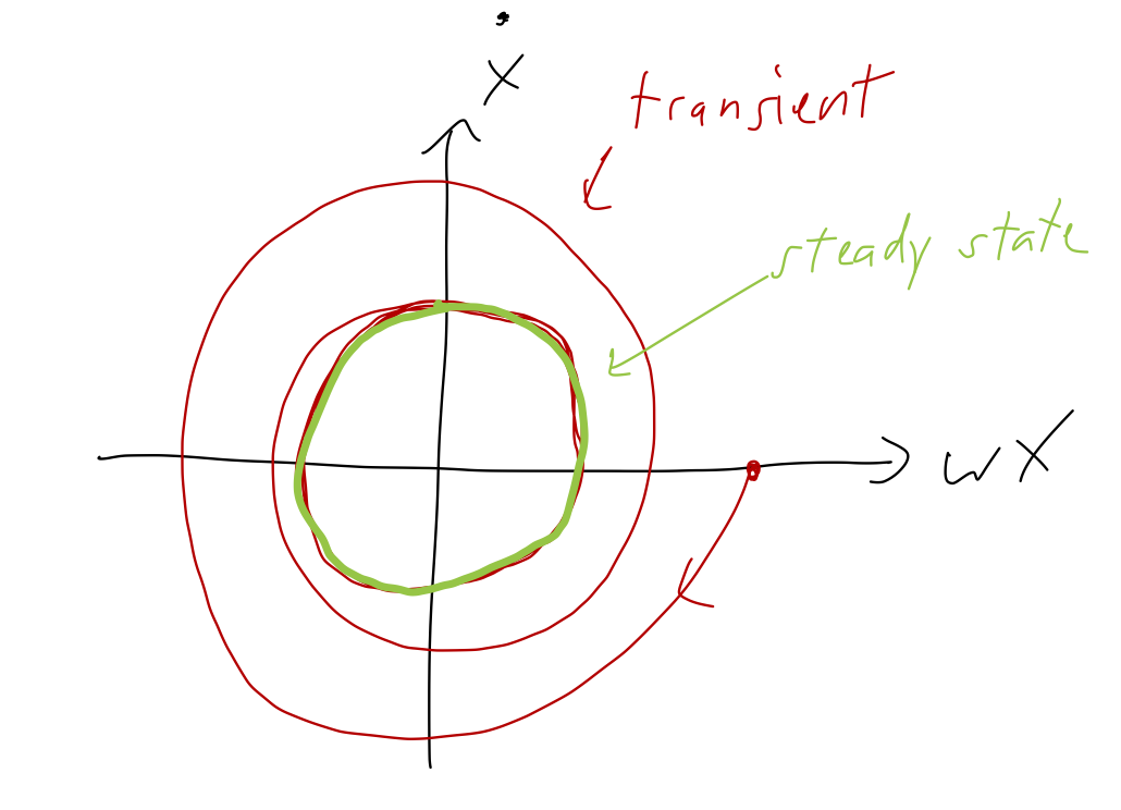
Let’s look at another special case to try to get a better feeling for this solution. Suppose that we have pure cosine driving F(t) = F_0 \cos (\omega t, and we’re in the underdamped case, \beta < \omega_0. Then we can write the full solution with driving in the form x(t) = A \cos (\omega t - \delta) + A_1 e^{-\beta t} \cos (\omega_1 t - \delta_1) This is a little complicated-looking, but the second part of the solution is known as the transient; more important than the oscillation, it dies off exponentially as t increases. So although the short-time behavior will include both components, if we wait long enough, the transient term vanishes and we’re just left with a simple oscillation at the driving frequency:
![]()
In fact, this is completely general: we know the critically damped and overdamped cases also die off exponentially with time, so those components are also transients. We find that no matter what \beta is, the long-term behavior of a driven damped oscillator is just simple oscillation at exactly the driving frequency.
Here, you should complete Tutorial 5E on “Damped and driven harmonic motion”. (Tutorials are not included with these lecture notes; if you’re in the class, you will find them on Canvas.)
5.4.3 Phase space and the driven oscillator
Let’s summarize what we’ve found. The key points to remember for sinusoidal (i.e. complex exponential) driving force F(t) = F_0 e^{i\omega t} are:
The long-term behavior is oscillation of the form x(t) \rightarrow A \cos (\omega t - \delta) at exactly the same angular frequency \omega as the driving force. At shorter times there will be an additional transient behavior, with form depending on whether the system is over/underdamped.
The motion of the system is phase shifted relative to the driving force, with phase shift given by \tan \delta = \frac{2\beta \omega}{\omega_0^2 - \omega^2}.
The amplitude of the system depends not just on the strength of the force, but also on the frequency of the driving, the natural frequency, and the damping constant: A = \frac{F_0/m}{\sqrt{(\omega_0^2 - \omega^2)^2 + 4\beta^2 \omega^2}}.
Actually, it’s useful to plug the first formula into the second to get another way of understanding the amplitude. We have, combining: A = \frac{F_0/m}{2 \beta \omega \sqrt{1 + \cot^2 \delta}} = \frac{F_0}{2\beta \omega m} \sin \delta.
So the amplitude will be maximized (roughly) when the phase shift is \delta = \pi/2 - roughly since we can’t adjust \delta independent of \omega, of course.
We can also think about a phase portrait as a visual way to understand the behavior of the damped, driven oscillator. Here I will be fairly qualitative, instead of going into too much mathematical detail. Once the transient behavior is gone and the system reaches steady-state, since x(t) takes the form of a simple harmonic oscillator, the phase portrait will be simple again: if we plot \omega x vs. \dot{x}, we will see a circle. However, there can be some additional evolution in phase space due to the transient, as the system moves from its initial conditions to the steady state.
For example, the evolution with underdamping and driving could look something like this:
We can recall that for the simple harmonic oscillator, the circular phase portrait was related to conservation of energy: the radius of the circle was proportional to \sqrt{E}. What about for the driven oscillator? In steady-state, we have \dot{x}(t) \rightarrow -\omega A \sin (\omega t - \delta) and so the total energy is E = \frac{1}{2}kx^2 + \frac{1}{2}m \dot{x}^2 \\ = \frac{1}{2} k A^2 \cos^2 (\omega t - \delta) + \frac{1}{2} m \omega^2 A^2 \sin^2 (\omega t - \delta) So far, same as the ordinary SHO. But the key difference here is that the driving frequency \omega is not (generally) the same as the natural frequency \omega_0! We can simplify further, using m\omega_0^2 = k: E = \frac{1}{2} kA^2 + \frac{1}{2} m (\omega^2 - \omega_0^2) A^2 \sin^2 (\omega t - \delta) So we have the expected constant energy term, plus a second term that oscillates. This might be puzzling at first glance; if we have steady-state motion, how can the energy possibly be changing?
The first thing we should observe is that although the energy changes, it is still periodic: if we wait for \Delta t = T = 2\pi/\omega, then E does stay exactly the same. So on average, the energy of the steady-state solution is not changing.
We can gain further insight by appealing to the work-KE theorem. Specifically, we recall that when the energy changes, the change is equal to the work done by all non-conservative forces, \Delta E = W_{\textrm{non-cons}}. So the second term must be the combined result of the work done by the two non-conservative forces here: the damping force and the driving force. It will vanish when \omega = \omega_0, which from above also gives us \delta = \pi/2 so that the driving force is perfectly in phase with the steady-state speed \dot{x}.
As we will see a bit later on, something else interesting happens here: when \omega \approx \omega_0, the amplitude A is maximized, holding all other properties of the system constant. We can try to tell a story related to energy: at any given instant, the work done by the damping dW_\beta on our oscillator is always negative (friction always dissipates energy.) On the other hand, the work done by the driving dW_d can be positive or negative, depending on whether it is aligned with the motion or not (the sign of work is controlled by the sign of F\dot{x}.) In general, some of the driver’s work is “wasted” by being negative; if we manage to line it up perfectly so that dW_d is always positive, then we get the maximum amplitude A out of our system.
We can try to go deeper into this story of energy and the driven oscillator, but the details get rather subtle, and we ultimately don’t need to work in terms of energy to understand the behavior of ampltiude vs. frequency - which we will get to under “Resonance” below. But this qualitative picture may help to guide your intuition about the driven oscillator, at least. For now, let’s move on to another topic.
5.5 Fourier series
So far, we’ve only solved two particular cases of driving force for the harmonic oscillator: constant, and sinusoidal (i.e. complex exponential.) The latter case is useful on its own, since there are certainly cases in which this is a good model for a real driving force. But it’s actually much more useful than it appears at first. This is thanks to a very powerful technique known as Fourier’s method, or more commonly, Fourier series.
Let’s think back to our earlier discussion of another important series method, which was power series. Recall that our starting point was to imagine a power-series representation of an arbitrary function f(x): f(x) = c_0 + c_1 x + c_2 x^2 + ... = \sum_{n=0}^{\infty} c_n x^n There are subtle mathematical issues about convergence and domain/range, as we noted. But putting the rigorous issues aside, the basic idea is that both sides of this equation are the same thing, hence the term “representation”. If we really keep an infinite number of terms, there is no loss of information when we go to the series - it is the function f(x).
Our starting point for Fourier series is very similar. We suppose that we can write a Fourier series representation of an arbitrary function f(t): f(t) = \sum_{n=0}^\infty \left[ a_n \cos(n \omega t) + b_n \sin (n \omega t) \right], where we now have two sets of arbitrary coefficients a_n and b_n, and \omega is a fixed angular frequency. Now, unlike the power-series representation, this actually can’t work for any f(t); the issue is that since we’re using sine and cosine, the series representation is now explicitly periodic, with period \tau = 2\pi / \omega. So for both sides of this equation to be the same, we must require that the function f(t) is also periodic, i.e. this is valid only if f(t + \tau) = f(t). (In other words, \omega is not something we pick arbitrarily - it comes from the periodicity of the function f(t) we’re trying to represent.) With this one important condition of periodicity, we now think of this just like a power-series representation: if we really keep an infinite number of terms, both sides of the equation are identical.
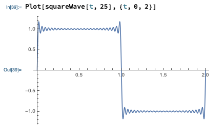
Two small, technical notes at this point. First, again if we went into detail on the mathematical side, we would find that there are certain requirements on the function f(t) for the Fourier series representation to converge properly - the function has to be “nice enough” for the series to work, roughly. The requirements for “nice enough” are weaker than you might expect; in particular, even sharp and discontinuous functions like a sawtooth or square wave admit Fourier series representations which converge at more or less every point. Here’s the Fourier series for a square wave, truncated at the first 25 terms (which might sound like a lot, but is really easy for a computer to handle:)
Second, you might wonder why we use this particular form of the series. Why not a power series in only cosine with phase shifts, or a power series in \cos(\omega t)^n instead of \cos(n \omega t)? The short answer is that these wouldn’t be any different - through trig identities, they’re related to the form I’ve written above. The standard form that we’ll be using makes it especially easy to calculate the coefficients a_n and b_n for a given function, as we shall see.
Now, in practice we can’t really compute the entire infinite Fourier series except in really special cases. This is just like power series: after this formal setup, in practice we will use the truncated Fourier series f_M(t) = \sum_{n=0}^{M} \left[ a_n \cos(n \omega t) + b_n \sin (n \omega t) \right] and adjust M until the error made by truncation is small enough that we don’t care about it.
Unlike power series, we don’t need to come up with any fancy additional construction to find a useful Fourier series. In fact, the basic definition is enough to let us calculate the coefficients of the series for any function. To get there, we need to start by playing with some integrals!
Let’s warm up with the following integral: \int_{-\tau/2}^{\tau/2} \cos (\omega t) dt = \left. \frac{1}{\omega} \sin (\omega t) \right|_{-\tau/2}^{\tau/2} \\ = \frac{1}{\omega} \left[ \sin\left( \frac{\omega \tau}{2} \right) - \sin\left( \frac{-\omega \tau}{2} \right) \right]. The fact that we’ve integrated over a single period lets us immediately simplify the result. By definition of the period, we know that \sin(\omega (t + \tau)) = \sin(\omega t + 2\pi) = \sin(\omega t). Since the difference between the two sine functions is exactly \omega \tau, they are equal to each other and cancel perfectly. So the result of the integral is 0. Similarly, we would find that \int_{-\tau/2}^{\tau/2} \sin (\omega t) = 0. Both of these simple integrals are just stating the fact that over the course of a single period, both sine and cosine have exactly as much area above the axis as they do below the axis.
This is a simple observation, but it’s important that we integrate for an entire period of oscillation to get zero as the result. (Some books will use the interval from 0 to \tau to define Fourier series instead, for example; everything we’re about to do works just as well for that convention.)
Now, what if we start combining trig functions together? The graphical context above suggests that if we square the trig functions and then integrate, we will no longer get zero, because they’ll be positive everywhere. Indeed, it’s straightforward to show that \int_{-\tau/2}^{\tau/2} \sin (\omega t) \sin (\omega t) dt = \int_{-\tau/2}^{\tau/2} \cos (\omega t) \cos (\omega t) dt = \frac{\pi}{\omega} = \frac{\tau}{2} (I am writing \sin^2 and \cos^2 suggestively as a product of two sines and cosines.) However, if we have one sine and one cosine, we instead get \int_{-\tau/2}^{\tau/2} \sin (\omega t) \cos (\omega t) dt = \int_{-\tau/2}^{\tau/2} \frac{1}{2} \sin (2\omega t) dt = 0 (this is now integrating over two periods for \sin(2\omega t) - zero twice is still just zero!)
So far, so good. But what if we start combining trigonometric functions of the more general form \sin (n \omega t), as appears in our Fourier series expansion? For example, what is the result of the integral \int_{-\tau/2}^{\tau/2} \sin(3 \omega t) \sin(5 \omega t) dt = ? We could painstakingly apply trig identities to break this down into a number of integrals over \sin(\omega t) and \cos (\omega t). However, a much better way to approach this problem is using complex exponentials. Let’s try this related complex-exponential integral first: \int_{-\tau/2}^{\tau/2} e^{3i\omega t} e^{5i \omega t} dt = \int_{-\tau/2}^{\tau/2} e^{8i \omega t} dt \\ = \left. \frac{1}{8i \omega} e^{8i \omega t} \right|_{-\tau/2}^{\tau/2} \\ = \frac{1}{8i \omega} \left[ e^{4i \omega \tau} - e^{-4i \omega \tau} \right] = 0 where as in our original example, we know that the complex exponentials are periodic, e^{i\omega (t + n\tau)} = e^{i \omega t}, so the terms in square brackets cancel off. No trig identities needed here!
Let’s do the fully general case for complex exponentials, to see whether there’s anything special about the numbers we’ve chosen here.
\int_{-\tau/2}^{\tau/2} e^{im\omega t} e^{in \omega t} dt = \int_{-\tau/2}^{\tau/2} e^{i(m+n)\omega t} dt \\ = \left. \frac{1}{(m+n)i \omega} e^{i(m+n)\omega t} \right|_{-\tau/2}^{\tau/2} \\ = \frac{1}{(m+n)i \omega} \left[ e^{i(m+n) \omega \tau/2} - e^{-i(m+n) \omega \tau/2} \right] \\ = \frac{1}{(m+n) i \omega} e^{i(m+n) \omega \tau} \left[1 - e^{-2\pi i(m+n)} \right], using \omega \tau = 2\pi on the last line. This is always zero, as long as m and n are both integers, since e^{2\pi i} is just 1. However, there is an edge case we ignored: if m = -n, then we have a division by zero. This is because we didn’t do the integral correctly in that special case: \int_{-\tau/2}^{\tau/2} e^{-in \omega t} e^{in \omega t} dt = \int_{-\tau/2}^{\tau/2} dt = \tau. We can write this result compactly using the following notation: \frac{1}{\tau} \int_{-\tau/2}^{\tau/2} e^{-im \omega t} e^{in \omega t} dt = \delta_{mn} where \delta_{mn} is a special symbol called the Kronecker delta symbol:
The Kronecker delta symbol \delta_{mn} is defined as:
\delta_{mn} = \begin{cases} 1, & m = n; \\ 0, & m \neq n. \end{cases}
In other words, the integral over a single period of two complex exponential functions e^{in\omega t} is always zero unless they have equal and opposite values of n and cancel off under the integral.
Now we’re ready to go back to the related integral that we started with, over products of sines and cosines. We can rewrite it using complex exponentials to apply our results: \int_{-\tau/2}^{\tau/2} \sin(3 \omega t) \sin(5 \omega t) dt = \int_{-\tau/2}^{\tau/2} \frac{1}{2i} \left( e^{3i\omega t} - e^{-3i\omega t}\right) \frac{1}{2i} \left( e^{5i \omega t} - e^{-5i \omega t} \right) dt \\ = -\frac{1}{4} \int_{-\tau/2}^{\tau/2} \left( e^{8i \omega t} - e^{-2i\omega t} - e^{2i \omega t} + e^{-8i \omega t} \right) dt \\ = 0, since none of the pairs of complex exponential terms cancel each other off. In fact, we can easily extend this to the general case: \int_{-\tau/2}^{\tau/2} \sin(m \omega t) \sin(n \omega t) dt = -\frac{1}{4} \int_{-\tau/2}^{\tau/2} \left( e^{im\omega t} - e^{-im \omega t} \right) \left( e^{in \omega t} - e^{-in \omega t} \right) dt \\ = -\frac{1}{4} \int_{-\tau/2}^{\tau/2} \left( e^{i(m+n)\omega t} + e^{-i(m+n) \omega t} - e^{i(m-n) \omega t} - e^{-i(m-n) \omega t}\right) dt Assuming m and n are both positive, the only way this will ever give a non-zero answer is if m=n, in which case we have -\frac{1}{4} \int_{-\tau/2}^{\tau/2} (-2 dt) = \frac{\tau}{2}. (If we had a negative m or n, we could use a trig identity to rewrite it, i.e. \sin(-m\omega t) = -\sin(m \omega t).) Again using the Kronecker delta symbol to write this compactly, we have the important result \frac{2}{\tau} \int_{-\tau/2}^{\tau/2} \sin (m \omega t) \sin (n \omega t) dt = \delta_{mn}. It’s not difficult to show that similarly, \frac{2}{\tau} \int_{-\tau/2}^{\tau/2} \cos (m \omega t) \cos (n \omega t) dt = \delta_{mn}, \\ \frac{2}{\tau} \int_{-\tau/2}^{\tau/2} \sin (m \omega t) \cos (n \omega t) dt = 0, again for positive (>0) integer values of m and n. (This last formula is obvious, even without going into complex exponentials: this is the integral of an odd function times an even function over a symmetric interval, so it must be zero.)
The combination of these three results is incredibly powerful when applied to a Fourier series! Recall that the definition of the Fourier series representation of a function f(t) was f(t) = \sum_{n=0}^\infty \left[ a_n \cos(n \omega t) + b_n \sin (n \omega t) \right]. Suppose we want to know what the coefficient a_4 is. Thanks to the integral formulas we found above, if we integrate the entire series against the function \cos(4 \omega t), the integral will vanish for every term except precisely the one we want: \frac{2}{\tau} \int_{-\tau/2}^{\tau/2} f(t) \cos(4 \omega t) dt \\ = \frac{2}{\tau} \sum_{n=0}^\infty \left[ a_n \int_{-\tau/2}^{\tau/2} \cos (n \omega t) \cos (4 \omega t) dt + b_n \int_{-\tau/2}^{\tau/2} \sin(n \omega t) \cos (4 \omega t) dt \right] \\ = \sum_{n=0}^{\infty} \left[ a_n \delta_{n4} + b_n (0) \right] = a_4.
In fact, we can now write down a general integral formula for all of the coefficients in the Fourier series: a_n = \frac{2}{\tau} \int_{-\tau/2}^{\tau/2} f(t) \cos(n \omega t) dt, \\ b_n = \frac{2}{\tau} \int_{-\tau/2}^{\tau/2} f(t) \sin(n \omega t) dt, \\ a_0 = \frac{1}{\tau} \int_{-\tau/2}^{\tau/2} f(t) dt, \\ b_0 = 0. The n=0 cases are special, and I’ve split them out: of course, b_0 is always multiplying the function \sin(0) = 0, so it doesn’t matter what it is - we can just ignore it. As for a_0, it is a valid part of the Fourier series, but it corresponds to a constant offset. We find its value by just integrating the function f(t); this integral is zero for any of the trig functions, but just gives back \tau on the constant a_0 term.
Let’s take a moment to appreciate the power of this result! To calculate a Taylor series expansion of a function, we have to compute derivatives of the function over and over until we reach the desired truncation order. These derivatives will generally become more and more complicated to deal with as they generate more terms with each iteration. On the other hand, for the Fourier series we have a direct and simple formula for any coefficient; finding a_{100} is no more difficult than finding a_1! So the Fourier series is significantly easier to extend to very high order.
Here, you should complete Tutorial 5F on “Fourier series”. (Tutorials are not included with these lecture notes; if you’re in the class, you will find them on Canvas.)
Let’s do a concrete and simple example of a Fourier series decomposition. Consider the following function which is periodic but always linearly increasing (this is sometimes called the sawtooth wave):
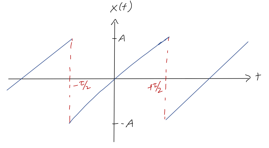
The equation describing this curve is x(t) = 2A\frac{t}{\tau},\ -\frac{\tau}{2} \leq t < \frac{\tau}{2}
Let’s find the Fourier series coefficients for this curve. Actually, we can save ourselves a bit of work if we think carefully first: all of the a_n must be equal to zero!
There are a couple of ways to see that all of the a_n for n>0 have to vanish (we’ll come back to a_0, which we generally have to think about separately.) First, we can just write out the integral for a_n using the definition of the sawtooth: a_n = \frac{4A}{\tau^2} \int_{-\tau/2}^{\tau/2} t \cos(n \omega t) dt. This integral is always zero, since \cos (n \omega t) is an even function for any n, but t is odd. We could also argue this directly from the Fourier series by observing that the sawtooth function itself is odd (within a single period \tau); this means that its series should only contain odd functions, meaning the \cos(n \omega t) parts should all be zero.
As for a_0, if we used the second argument above then odd-ness of the sawtooth tells us a_0 = 0 too. If we used integrals, we can just write out the integral again to find a_0 = \frac{1}{\tau} \int_{-\tau/2}^{\tau/2} x(t) dt = \frac{1}{\tau} \int_{-\tau/2}^{\tau/2} \frac{2A}{\tau} t\ dt = 0. We can also read this off the graph: a_0 is just the average value of the function over a single period, which is clearly zero.
The above observation is something we should always look for when computing Fourier series: if the function to be expanded is odd, then all of the a_n will vanish (including a_0), whereas if it is even, all the b_n will vanish instead.
On to the integrals we actually have to compute: b_n = \frac{4A}{\tau^2} \int_{-\tau/2}^{\tau/2} t \sin(n \omega t) dt This is a great candidate for integration by parts. Rewriting the integral as \int u dv, we have u = t \Rightarrow du = dt \\ dv = \sin (n \omega t) dt \Rightarrow v = -\frac{1}{n \omega} \cos (n \omega t) and so \int u\ dv = uv - \int v\ du \\ = \left. -\frac{1}{n \omega} t \cos (n \omega t) \right|_{-\tau/2}^{\tau/2} + \frac{1}{n \omega} \int_{-\tau/2}^{\tau/2} \cos(n \omega t) dt \\ = -\frac{1}{n \omega} \left[ \frac{\tau}{2} \cos (n\pi) - \frac{-\tau}{2} \cos (-n\pi) \right] + \frac{1}{n^2 \omega^2} \left[ \sin (n \pi) - \sin (-n\pi) \right] The second term just vanishes since \sin(n\pi) = 0 for any integer n. As for the first term, \cos(n\pi) is either +1 if n is even, or -1 if n is odd. Since \cos(-n\pi) = \cos(n\pi), we have the overall result \int u\ dv = -\frac{1}{n\omega} \left[ \frac{\tau}{2} (-1)^n + \frac{\tau}{2} (-1)^n \right] = -\frac{\tau}{n \omega} (-1)^n, or plugging the integral back into the Fourier coefficient formula, b_n = \frac{4A}{\tau^2} \int u\ dv = \frac{-4A \tau}{n \omega \tau^2} (-1)^n = -\frac{2A}{\pi n} (-1)^n = \frac{2A}{\pi n} (-1)^{n+1}, absorbing the overall minus sign at the very end. And now we’re done - we have the entire Fourier series, all coefficients up to arbitrary n as a simple formula! Once again, you can appreciate how much easier it is to keep many terms before truncating in this case, compared to using a Taylor series. Plugging in some numbers to get a feel for this, the first few coefficients are b_1 = \frac{2A}{\pi},\ b_2 = -\frac{A}{\pi}, b_3 = \frac{2A}{3\pi}, b_4 = -\frac{A}{2\pi}, ... Importantly, the size of the coefficients is shrinking as n increases, due to the 1/n in our formula. Unlike the Fourier series, there is no automatic factor of 1/n! to help with convergence, so we should worry a little about the accuracy of truncating a Fourier series! It is, nevertheless, quite generic for the size of the Fourier series coefficients to die off in some way with n. Remember that we’re building a function up out of sines and cosines. Functions like \cos(n \omega t) with n very large are oscillating very, very quickly; if the function we’re building up is relatively smooth, it makes sense that the really fast-oscillating terms won’t be very important in modeling it.
Let’s plug in some numbers and get a feel for how well our Fourier series does in approximating the sawtooth wave! Choosing A=1 and \omega = 2\pi (so \tau = 1), here are some plots keeping the first m terms before truncating:
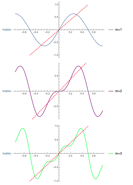
We can see that even as we add the first couple of terms, the approximation of the Fourier series curve to the sawtooth (the red line, plotted just for the region from -\tau/2 to \tau/2) is already improving rapidly.
To visualize a bit better what’s happening here, let’s look at the three separate components of the final m=3 curve:
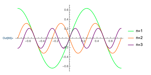
We clearly see that the higher-n components are getting smaller. If you compare the two plots, you can imagine “building up” the linear sawtooth curve one sine wave at a time, making finer adjustments at each step.
Of course, although m=3 might be closer to the sawtooth than you expected, it’s still not that great - particularly near the edges of the region. Since we have an analytic formula, let’s jump to a nice high truncation of m=50:
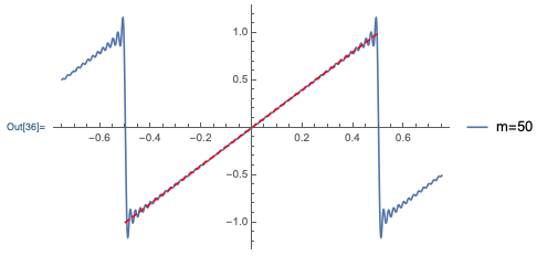
This is a remarkably good approximation - it’s difficult to see the difference between the Fourier series and the true curve near the middle of the plot! At the discontinuities at \pm \tau/2, things don’t work quite as well; we see the oscillation more clearly, and the Fourier series is overshooting the true amplitude by a bit. In fact, this effect (known as the Gibbs phenomenon) persists no matter how many terms we keep: there is a true asymptotic (n \rightarrow \infty) error in the Fourier series approximation whenever our function jumps discontinuously, so we never converge to exactly the right function.
The good news is that as we add more terms, this overshoot gets arbitrarily close to the discontinuity (the Gibbs phenomenon gets narrower), so we can still improve our approximation in that way. We’ll always be stuck with this effect at the discontinuity, but of course real-world functions don’t really have discontinuities, so this isn’t really a problem in practice.
We could try to look at a plot of all of the 50 different sine waves that build up the m=50 sawtooth wave above, but it would be impossible to learn anything from the plot because it would be too crowded. Instead of looking at the whole sine waves, a different way to visualize the contributions is just to plot the coefficients |b_n| vs. n:
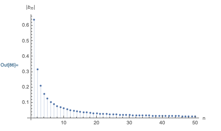
The qualitative 1/n behavior of the coefficients is immediately visible. This plot is sometimes known as a frequency domain plot, because the n on the horizontal axis is really a label for the size of the sine-function components with frequency n\omega. If we didn’t have a simple analytic formula and had to do the integrals for the a_n and b_n numerically, such a plot gives a simple way to check at a glance that the Fourier series is converging.
We’ll only do this one example in lecture, but have a look in Taylor for a second example of finding the Fourier coefficients of a simple periodic function.
5.5.1 Solving the damped, driven oscillator with Fourier series
Now we’re ready to come back to our physics problem: the damped, driven oscillator. Suppose now that we have a totally arbitrary driving force F(t), which is periodic with period \tau: \ddot{x} + 2\beta \dot{x} + \omega_0^2 x = \frac{F(t)}{m} Since F(t) is periodic, we can find a Fourier series decomposition: F(t) = \sum_{n=0}^\infty \left[ a_n \cos (n \omega t) + b_n \sin (n \omega t) \right] As we saw before, if the driving force consists of multiple terms, we can just solve for one particular solution at a time and add them together. So in fact, we know exactly how to solve this already! The particular solution has to be x_p(t) = \sum_{n=0}^\infty \left[ A_n \cos (n \omega t - \delta_n) + B_n \sin (n \omega t - \delta_n) \right] where the amplitudes and phase shifts for each term are exactly what we found before, just using n \omega as the driving frequency: A_n = \frac{a_n/m}{\sqrt{(\omega_0^2 - n^2\omega^2)^2 + 4\beta^2 n^2 \omega^2}} \\ B_n = \frac{b_n/m}{\sqrt{(\omega_0^2 - n^2\omega^2)^2 + 4\beta^2 n^2 \omega^2}} \\ \delta_n = \tan^{-1} \left( \frac{2\beta n \omega}{\omega_0^2 - n^2 \omega^2} \right) At long times, this is the full solution: at short times, we add in the transient terms due to the complementary solution. (Note that the special case n=0, corresponding to a constant driving piece F_0, doesn’t require a different formula - it’s covered by the ones above, as you can check!)
So at the minor cost of finding a Fourier series for the driving force, we can immediately write down the solution for the corresponding driven, damped oscillator!
One extra point worth making here: remember that the energy of a simple harmonic oscillator is just E = \frac{1}{2} kA^2. At long times, when the system reaches its steady state, the Fourier decomposition tells us that it is nothing more than a combination of lots of simple harmonic oscillators! Thus, we can easily find the total energy by just adding up all of the individual contributions.
5.5.2 A useful analogy: Fourier series and vector spaces
Before we continue with more physics, I want to say more about the new symbol we introduced above, the Kronecker delta symbol. We actually could have introduced this symbol all the way back at the beginning of the semester, when we were talking about vector coordinates. Remember that for a general three-dimensional coordinate system, we can expand any vector in terms of three unit vectors: \vec{a} = a_1 \hat{e}_1 + a_2 \hat{e}_2 + a_3 \hat{e}_3. The dot product of any two vectors is given by multiplying the components for each unit vector in turn: \vec{a} \cdot \vec{b} = (a_1 \hat{e}_1 + a_2 \hat{e}_2 + a_3 \hat{e}_3) \cdot (b_1 \hat{e}_1 + b_2 \hat{e}_2 + b_3 \hat{e}_3) \\ = a_1 b_1 + a_2 b_2 + a_3 b_3. What if we just take dot products of the unit vectors themselves, so a_i and b_i are either 1 or 0? We immediately see that we’ll get 1 for the dot product of any unit vector with itself, and 0 otherwise, for example \hat{e}_1 \cdot \hat{e}_1 = 1, \\ \hat{e}_1 \cdot \hat{e}_3 = 0, and so on. The compact way to write this relationship is using the Kronecker delta again: \hat{e}_i \cdot \hat{e}_j = \delta_{ij}. This leads us to a technical math term that I didn’t introduce before: the set of unit vectors \{\hat{e}_1, \hat{e}_2, \hat{e}_3\} form an orthonormal basis. “Basis” here means that we can write any vector at all as a combination of the unit vectors. Orthonormal means that all of the unit vectors are mutually perpendicular, and they all have length 1. Saying that the dot products of the unit vectors is given by the Kronecker delta is the same thing as saying they are orthonormal! Orthonormality is a useful property because it’s what allows us to write the dot product in the simplest way possible.
Now let’s imagine a fictitious space that has more than 3 directions, let’s say some arbitrary number N. We can use the same language of unit vectors to describe that space, and once again, it’s most convenient to work with an orthonormal basis. It’s really easy to extend what we’ve written above to this case! We find a set of vectors \{\hat{e}_1, \hat{e}_2, ..., \hat{e}_N\} that form a basis, and then ensure that they are orthonormal, which is still written in exactly the same way, \hat{e}_i \cdot \hat{e}_j = \delta_{ij}. We can then expand an arbitrary vector out in terms of unit-vector components, \vec{a} = a_1 \hat{e}_1 + a_2 \hat{e}_2 + ... + a_N \hat{e}_N. Larger vector spaces like this turn out to be very useful, even for describing the real world. You’ll have to wait until next semester to see it, but they show up naturally in describing systems of physical objects, for example a set of three masses all joined together with springs. Since each individual object has three coordinates, it’s easy to end up with many more than 3 coordinates to describe the entire system at once.
Let’s wrap up the detour and come back to our current subject of discussion, which is Fourier series. This example is partly meant to help you think about the Kronecker delta symbol, but the analogy between Fourier series and vector spaces actually goes much further than that. Recall the definition of a (truncated) Fourier series is f_M(t) = a_0 + \sum_{n=1}^M \left[a_n \cos (n \omega t) + b_n \sin (n \omega t) \right]. Expanding the function f(t) out in terms of a set of numerical coefficients \{a_n, b_n\} strongly resembles what we do in a vector space, expanding a vector out in terms of its vector components. We can think of rewriting the Fourier series in vector-space language, f_M(t) = a_0 \hat{e}_0 + \sum_{n=1}^M \left[ a_n \hat{e}_n + b_n \hat{e}_{M+n} \right] defining a set of 2M-1 “unit vectors”, \hat{e}_0 = 1, \\ \hat{e}_{n} = \begin{cases} \cos(n \omega t),& 1 \leq n \leq M; \\ \sin(n \omega t),& M+1 \leq n \leq 2M; \end{cases} As you might suspect, the “dot product” (more generally known as an inner product) for this “vector space” is defined by doing the appropriate integral for the product of unit functions: \hat{e}_m \cdot \hat{e}_n = \frac{2}{\tau} \int_{-\tau/2}^{\tau/2} (\hat{e}_m) (\hat{e}_n) dt = \delta_{mn}. So our “unit vectors” are all orthonormal, and the claim that we can do this for any function f(t) means that they form an orthonormal basis!
I should emphasize that the space of functions is not really a vector space - mathematically, there are important differences. But there are enough similarities that this is a very useful analogy for conceptually thinking about what a Fourier series means. Just like a regular vector space, the Fourier series decomposition is nothing more than expanding the “components” of a periodic function in terms of the orthonormal basis given by \cos(n\omega t) and \sin(n \omega t). (Unlike a regular vector space, and more like a Taylor series, the contributions from larger n tend to be less important, so we can truncate the series and still get a reasonable answer. In a regular vector space, there’s no similar reason to truncate our vectors!)
Before we actually go into a detailed numerical solution for a driven oscillator, in order to better understand the physics of our solution, we need to first discuss the concept of resonance.
5.6 Resonance
Resonance is an interesting phenomenon which occurs in cases where the damping is relatively weak compared to both of the other frequencies, \beta \ll \omega, \omega_0. Resonance can be thought of as something which occurs when we vary the frequency and look at the amplitude of oscillations. In fact, we can see the effect qualitatively just from the amplitude formula we found. The denominator is \sqrt{(\omega_0^2 - \omega^2)^2 + 4 \beta^2 \omega^2} If \beta is relatively small, then we see that whenever \omega \approx \omega_0, the denominator is close to zero, which means the amplitude will be very large. We can think of this as a phenomenon which occurs either when varying \omega or varying \omega_0, with both cases being appropriate for different physical systems:
As we’ve referred to before, an LRC circuit is a common example of a damped oscillator. When a radio station broadcasts its signal, it does so at a fixed frequency \omega - the radio signal is the driving force in the LRC case. To listen to the radio, you tune your radio to change \omega_0, by adjusting the resistance or capacitance of your radio circuit. So in this case, \omega is fixed and we should think about changing \omega_0.
On the other hand, a real-world mechanical system like a bridge might have a certain natural frequency \omega_0 which is not easily adjusted. However, a person walking across the bridge provides a driving force with adjustable frequency \omega. So now we think of \omega_0 as fixed and imagine changing \omega.
Since \omega appears twice in the denominator, the simpler case will be when we hold it fixed and vary \omega_0. But for small enough \beta, the behavior (i.e. the phenomenon of resonance) will be the same in both cases.
Here, you should complete Tutorial 5G on “Resonance and the driven oscillator”. (Tutorials are not included with these lecture notes; if you’re in the class, you will find them on Canvas.)
Let’s think about the small-\beta limit, although we have to be careful with how we expand: we want to avoid actually taking \beta all the way to zero. As long as \beta^2 is small compared to either \omega^2 or \omega_0^2, we see that the second term underneath the square root is always very small. Meanwhile, the first term will also become small if we let \omega_0 \rightarrow \omega. Once both terms are small, the overall amplitude will become very large - diverging, in fact, if we really try to set \beta = 0.
Let’s factor out a 1/\omega^2 from everything, resulting in A = \frac{F_0/m}{\omega^2 \sqrt{(1 - \omega_0^2 / \omega^2)^2 + 4 \beta^2 / \omega^2 }}. Now we series expand as \omega_0 / \omega \rightarrow 1. As usual, this is easier if we change variables: let’s say that \omega_0 = \omega + \epsilon. Then (1 - \omega_0^2 / \omega^2)^2 = (1 - (1 - \epsilon/\omega)^2)^2 = (1 - 1 + 2\epsilon/\omega - \epsilon^2/\omega^2)^2 \approx 4\epsilon^2/\omega^2 discarding higher-order terms in \epsilon. Then series expanding with the binomial formula gives A = \frac{F_0/m}{\omega \sqrt{4\epsilon^2 + 4\beta^2}} \\ = \frac{F_0}{2\omega m} \left( \frac{1}{\beta} - \frac{\epsilon^2}{2\beta^3} + ...\right)
So close to \omega_0 = \omega, we have a local maximum amplitude of A = F_0 / (2m \omega \beta). Near this maximum, as we change \omega_0 slightly away from \omega, the amplitude decreases quadratically. In fact, it’s easy to see that this peak is the global maximum: any value of \omega_0 different from \omega gives a positive contribution to the denominator and makes A smaller.
Moving away from the peak, we see furthermore that as \omega_0 \rightarrow 0 the amplitude goes to a finite value, A(\omega_0 \rightarrow 0) \rightarrow \frac{F_0/m}{\omega^2 \sqrt{1 + 4\beta^2 / \omega^2}} \approx \frac{F_0}{m \omega^2} using the fact that we’re in the weak-damping limit so \beta / \omega is small. This also tells us that this value of A is much smaller than the peak, again by one power of \beta / \omega. Finally, going to large natural frequency, the \omega_0^4 term eventually dominates everything else, and we find A(\omega_0 \rightarrow \infty) \rightarrow \frac{F_0}{m \omega_0^2}, which dies off to zero as \omega_0 gets larger and larger. Now we have all the information we need to make a sketch of amplitude vs. natural frequency:
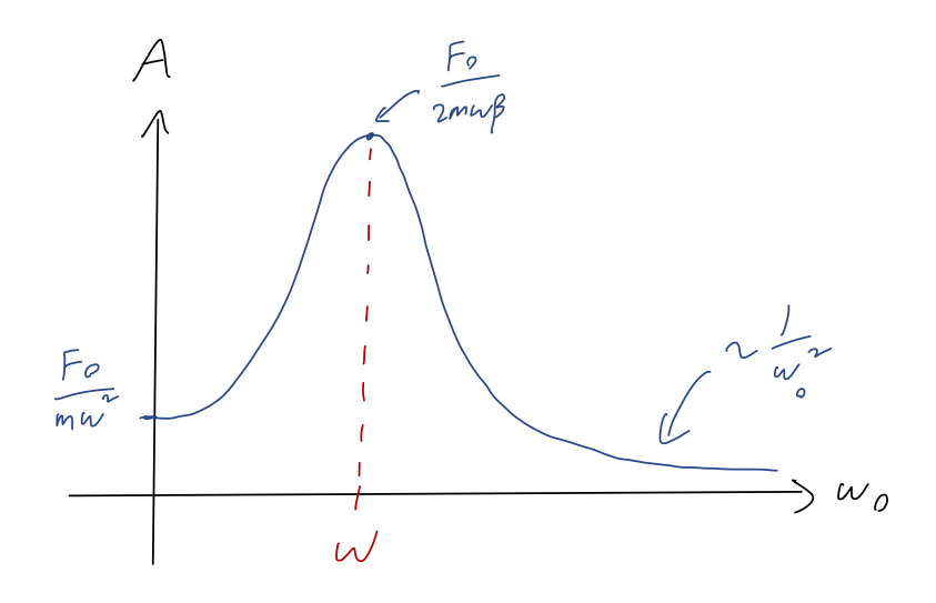
The large peak in the amplitude is called a resonance. Basically, we obtain a huge increase in the amplitude of oscillations as we tune the natural frequency \omega_0 close to the driving frequency \omega. This effect is stronger when \beta is small: as \beta decreases, the peak amplitude becomes larger and the resonance becomes sharper (the width decreases.)
Now let’s briefly consider the alternative situation, where \omega_0 is fixed and we are instead adjusting the driving frequency \omega. This will be a lot messier if we try to series expand, but we know that we expect the same qualitative behavior: as the term \omega_0 - \omega vanishes in the denominator, the amplitude will become very large as long as the second term including \beta is relatively small. Instead of doing the full series expansion, let’s use a derivative to find the position of the resonance peak. It will be easier to work with the squared amplitude for this:
|A|^2 = \frac{F_0^2/m^2}{(\omega_0^2 - \omega^2)^2 + 4\beta^2 \omega^2} (it should be clear that the maximum of |A| is also the maximum of |A|^2.) We can take a derivative of the whole thing to find extrema, but maximizing |A|^2 is the same thing as minimizing the denominator alone, so let’s just work with that directly: \frac{d}{d\omega} \left[ (\omega_0^2 - \omega^2)^2 + 4\beta^2 \omega^2 \right] = -4 \omega (\omega_0^2 - \omega^2) + 8\beta^2 \omega = 0 This has a solution at \omega = 0, but we know already that’s not the right answer for the resonance peak. Dividing out the overall \omega leaves us with a quadratic equation, 4 \omega^2 - 4\omega_0^2 + 8 \beta^2 = 0 \\ \omega = \sqrt{\omega_0^2 - 2\beta^2} taking the positive root since \omega has to be positive. This is close to \omega_0 for small \beta, so this is definitely the location of the resonance peak! We notice that in this case, there’s actually a small offset: the peak as a function of \omega is slightly to the left of \omega = \omega_0.
Let’s make another sketch here, using the behavior we just found; we’ll also need to know what happens as \omega \rightarrow 0. In the latter case, we can just plug in directly and not even worry about expanding anything to find A(\omega \rightarrow 0) = \frac{F_0}{m\omega_0^2}.
Thus, the sketch of amplitude for varying \omega looks like this:
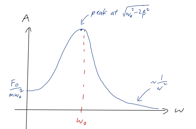
If we plug back in the peak value into the amplitude formula, we find A = \frac{F_0/m}{\sqrt{(\omega_0^2 - (\omega_0^2 - 2\beta^2))^2 + 4\beta^2 (\omega_0^2 - 2\beta^2)}} \\ = \frac{F_0/m}{\sqrt{4 \beta^2 (\omega_0^2 - \beta^2)}} \approx \frac{F_0}{2m\omega_0 \beta} neglecting the extra term proportional to (\beta/\omega_0)^2. This is the same as in the case where we varied \omega_0.
In addition to the height of the resonance peak, the width of the resonance is also an important quantity to know. We argued from our series expansion before that small \beta means narrower width, since the quadratic term in (\omega - \omega_0) gets steeper at smaller \beta. Let’s be a little more quantitative and ask about the full-width at half maximum, or FWHM. By convention, this is defined for the value of the squared amplitude, |A|^2 (which is proportional to the energy, recall: E = \frac{1}{2} k|A|^2.)
Let’s be clever about this. Recall that the squared amplitude is equal to |A|^2 = \frac{F_0^2/m^2}{(\omega_0^2 - \omega^2)^2 + 4\beta^2 \omega^2}. Now, the peak occurs roughly where the first term vanishes, leaving just the second term. Therefore, the half-max value is where the first term is equal to the second term, so the denominator becomes 8\beta^2 \omega^2. Setting these equal gives (\omega_0^2 - \omega_{\textrm{HM}}^2)^2 = 4\beta^2 \omega_{\textrm{HM}}^2 \\ \omega_0^2 - \omega_{\textrm{HM}}^2 \approx \pm 2\beta \omega_{\textrm{HM}}. This is easy to solve since it’s a quadratic equation, although we need to be a little careful with which roots we keep. Using the quadratic formula, we find \omega_{\textrm{HM}} = \mp \beta \pm \sqrt{\beta^2 + \omega_0^2} (all four combinations of signs appear, because we have two minus signs and then two roots for each.) Now, since we’re working where \beta \ll \omega_0, the \beta^2 under the root is completely negligible, and the second term is just \pm \omega_0. This must be +\omega_0, in fact, because \omega_{\textrm{HM}} has to be positive. Thus, we find our approximate answer \omega_{\textrm{HM}} = \omega_0 \pm \beta. So we see explicitly that at roughly a difference in frequency of \beta on either side of the peak, the squared amplitude is reduced by half. The smaller \beta is, the sharper our resonance peak will be (and the larger the peak amplitude will be, as we already found.)
5.6.1 Quality factor
One more quantity that is conventionally defined in the context of resonance is the quality factor or Q-factor, denoted by Q. This is defined to be Q \equiv \frac{\omega_0}{2\beta} so it is a dimensionless number. This must be a number much larger than 1 under our assumptions, and the larger Q is, the sharper the resonance peak will be.
We can rewrite the peak resonance amplitude in terms of Q: recall that we had |A| \approx \frac{F_0}{2m\omega_0 \beta} = \frac{F_0}{m\omega_0^2} Q.
So a sharp peak also means a much higher peak for large Q, given the same amplitude of the driving force.
Essentially, Q is a comparison of the natural frequency of the resonator to the damping factor (which is, of course, also a frequency.) These correspond to two important physical timescales: T = 2\pi / \omega_0 determines the frequency of oscillation of the undriven oscillator, whereas since the amplitude dies off as e^{-\beta t} due to damping, \tau = 1/\beta gives the natural time for the decay of the amplitude. We can rewrite Q in terms of these timescales as Q = \frac{2\pi/T}{2/\tau} = \frac{\pi \tau}{T}. So a large Q means that a large number of oscillation periods T fit within a single decay time \tau. In other words, if we turn the driving force off, a high-Q resonator will continue to oscillate for a long time, losing energy very slowly to the damping.
Let’s summarize what we’ve found. (There is one more small observation we can make about the phase shift \delta; it changes rapidly near a resonance. But I don’t have much to say about the phase shift in this context, so I’ll let you read about it in Taylor.) For a weakly damped driven oscillator, a resonance peak occurs for \omega_0 \approx \omega. The amplitude at this peak is |A| \approx \frac{F_0}{2m\omega_0 \beta} = \frac{F_0}{m \omega_0^2} Q. The full-width at half-maximum is at approximately \omega = \omega_0 \pm \beta. The peak location as a function of \omega is actually slightly to the left of \omega_0, at \omega = \omega_{\textrm{peak}} = \sqrt{\omega_0^2 - 2\beta^2}. If instead we vary \omega_0 and hold \omega fixed, the resonance peak is exactly at \omega_0 = \omega. Finally, this is all focused on the long-time behavior, i.e. just the particular solution! There is also a transient oscillation which occurs at short times; since we are in the underdamped regime, the frequency of the transient oscillations is \omega_1 = \sqrt{\omega_0^2 - \beta^2} (not to be confused with \omega_{\textrm{peak}}!)
5.6.2 Resonance and Fourier series solutions
Everything we said about resonance remains true for this more general case of a driving force. The key difference is that while our object still has a single natural frequency \omega_0, we now have multiple driving frequencies \omega, 2\omega, 3\omega... all active at once! As a result, if we drive at a low frequency \omega \ll \omega_0, we can still encounter resonance as long as n\omega \approx \omega_0 for some integer value n. This effect is balanced by the fact that the amplitude of the higher modes is dying off as n increases, but since the effect of resonance is so dramatic, we’ll still see some effect from the higher mode being close to \omega_0.
(A simple everyday example of this effect is a playground swing, which typically has a natural frequency of roughly \omega_0 \sim 1 Hz. If you are pushing a child on a swing, and you try to push at a higher frequency than \omega_0, you won’t be very successful - all of the modes of your driving force are larger than \omega_0, so no resonance. On the other hand, pushing less frequently can still work, as long as n \omega \sim \omega_0, e.g. pushing them once every 3 or 4 seconds will still lead to some amount of resonance.)
Let’s see how this works by putting our previous example to work.
Suppose we have a driving force which is described well by a sawtooth wave, the same function that we found the Fourier series for above: F(t) = 2F_0 \frac{t}{\tau},\ -\frac{\tau}{2} \leq t \leq \frac{\tau}{2}.
What is the response of a damped, driven oscillator to this force?
Our starting point is finding the Fourier series to describe F(t), but we already did that: we know that a_n = 0 and b_n = \frac{2F_0}{\pi n} (-1)^{n+1}. Thus, applying our solution for the damped driven oscillator, we have for the particular solution x_p(t) = \sum_{n=0}^\infty B_n \sin(n \omega t - \delta_n) where B_n = \frac{2(-1)^{n+1} F_0/m}{\pi n\sqrt{(\omega_0^2 - n^2 \omega^2)^2 + 4\beta^2 n^2 \omega^2}}, \\ \delta_n = \tan^{-1} \left( \frac{2\beta n\omega}{\omega_0^2 - n^2 \omega^2} \right).
If we want the full solution, we add in whatever the corresponding complementary solution is. For example, if the system is underdamped (\beta < \omega_0), then x(t) = A e^{-\beta t} \cos (\sqrt{\omega_0^2 - \beta^2} t - \delta) + x_p(t) with A and \delta determined by our initial conditions. This solution is nice and easy to write down, but very difficult to work with by hand, particularly if we want to keep more than the first couple of terms in the Fourier series! To make further progress, let’s pick some numerical values and use Mathematica to make some plots. Let’s keep it underdamped so we can think about resonance; I’ll take \omega_0 = 1 to start and \beta = 0.2. Let’s also set F_0/m = 1 for simplicity. Finally, we’ll consider two values of the driving frequency \omega. Let’s begin with a higher driving frequency than the natural frequency, \omega = 3:
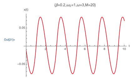
(Note that this is only the particular solution x_p(t), so this is the behavior at some amount of time after t=0 when the transient solution is gone.) Here I’m keeping M=20 terms in the Fourier series. This looks surprisingly simple given the complex shape of the driving force! Why is that? We can find a clue if we look in “frequency space” once again, i.e. if we plot the ampltiudes B_n of each of the Fourier coefficients:
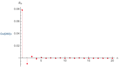
So the reason that the long-time response is so simple-looking is because there is a single Fourier component which is completely dominant; the first component, B_1. This comes in part from the Fourier series for the sawtooth wave force itself; we know the coefficients b_n of the force die off proportional to 1/n. But there’s another effect which is just as important. Remember that the Fourier series for the response is a sum of contributions at frequencies n \omega, i.e. at integer multiples of the fundamental driving frequency. Going back to our discussion of resonance, let’s think about where the first few frequencies lie on the resonance curve A(\omega):
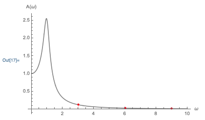
The black curve shows the resonance curve that we’ve considered before for simple sine-wave inputs. But now from the sawtooth force, we have multiple terms at \omega, 2\omega, 3\omega... = 3, 6, 9... that all contribute. But since we start at \omega much larger than \omega_0, all of the contributions from this sawtooth force are out on the tail of the resonance curve, which gives an additional suppression of the higher-frequency terms. In fact, if we go back to the formula we found for B_n, we see that B_n \propto 1/n^2 for n \omega \gg \omega_0.
This is a nice picture, and it should make you suspect that we will get a dramatically different result if we pick a driving frequency which is lower than \omega_0. Here’s our solution once again, with all of the same physical inputs except that \omega = 0.26/s:
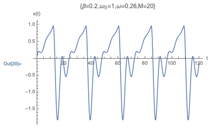
Now we can see some remnant of the sawtooth shape here in the response, although it’s far from perfect - we see especially complicated behavior at the ends of the cycle, where the force direction changes suddenly. As you can probably guess already, there are many more significant Fourier modes in the particular solution here. Here’s a plot of B_n for this case:
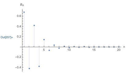
This time, several low-lying modes are important - in fact, the first few modes after B_1 are larger than they are in the sawtooth wave itself! Once again, we can easily understand what is happening in terms of the resonance curve:
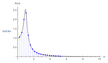
Since the fundamental driving force \omega < \omega_0 this time, we see that the first few multiples actually have their amplitudes enhanced by the resonance at \omega \approx \omega_0. This causes them to die off more slowly than the 1/n coming from the input force itself. Eventually, the higher frequencies move past the resonance, and we find the same 1/n^2 dependence as in the previous case. But if we had an even lower driving frequency, we might see a large number of Fourier modes contributing significantly.
The simple take-away message is that, for an underdamped oscillator, the system “wants” to resonate at the natural frequency \omega_0. If we drive at a lower frequency than \omega_0, we will tend to get several Fourier modes that contribute in the long-term behavior, and an interesting and complicated response. If instead we try to drive at a higher frequency than \omega_0, the response dies off very rapidly as frequency increases, so we get a response dominantly at the driving frequency itself. (Notice also that this response is much smaller in amplitude than the one that picks up the resonance - compare the amplitudes on the two x(t) plots above!)
5.7 Non-periodic forces and the driven oscillator
Clearly, Fourier series are a very powerful method for dealing with a wide range of driving forces in the harmonic oscillator. However, we are still restricted to considering only periodic driving forces. This is useful for a number of physical systems, but in the real world there are a larger number of examples in which the driving force is not periodic at all.
In fact, a simple example of a non-periodic driving force that has many practical applications is the impulse force:
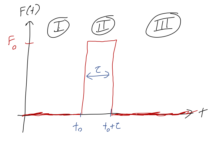
This force is zero everywhere, except for a small range of time extending from t_0 to t_0 + \tau, where \tau is the duration of the step, over which it has magnitude F_0. This is a decent model for most forces that you would apply yourself, without any tools: kicking a ball, or pushing a rotor into motion.
The easiest way to solve this problem is to break it into parts. Let’s suppose that we begin at rest, so x(0) = \dot{x}(0) = 0. Let’s also assume the system is underdamped - as usual, this gives the most interesting motion, since overdamped systems tend to just die off exponentially no matter what. Let’s analyze things based on the regions, marked I, II, III on the sketch. For t < t_0, we have the general solution x_I(t) = A e^{-\beta t} \cos (\omega_1 t - \delta) with \omega_1 = \sqrt{\omega_0^2 - \beta^2} as usual. Since the force is zero up until t=t_0, in this region there is no particular solution. Let’s apply our initial conditions: x_I(0) = A \cos (-\delta) = 0 \\ \dot{x}_I(0) = -\beta A \cos(-\delta) - \omega_1 A \sin(-\delta) = 0 Now, to solve the first equation we either have A = 0 or \delta = \pi/2. But if we try to use \delta = \pi/2, the second equation becomes \omega_1 A = 0 anyway. So in this region we just have A = 0, and there is no motion at all - not surprising, since there is no applied force and the oscillator starts at rest!
Next, let’s consider what happens during the step, for t_0 < t < t_0 + \tau. Here we have a constant driving force, which as we found before gives us a particular solution which is also constant, so we now have a slightly different general solution, x_{II}(t) = A' e^{-\beta t} \cos (\omega_1 t - \delta') + \frac{F_0}{m\omega_0^2}. Now, we can think of applying our initial conditions. Since our region starts at t=t_0, the initial condition is actually a boundary condition; we impose the requirement that the final position and speed of x_I(t) have to match the initial position and speed of x_{II}(t). Mathematically, we write this as x_I(t_0) = x_{II}(t_0) \\ \dot{x}_I(t_0) = \dot{x}_{II}(t_0) Now, since x_I(t) is just zero everywhere, this turns out to be the same initial conditions that we started with. But I’m writing this out carefully now, because we’ll need to match the boundary conditions again at the right-hand side to find x_{III}(t). Let’s apply the boundary conditions: x_{II}(t_0) = 0 = A' e^{-\beta t_0} \cos (\omega_1 t_0 -\delta') + \frac{F_0}{m\omega_0^2} \\ \dot{x}_{II}(t_0) = 0 = -\beta A' e^{-\beta t_0} \cos (\omega_1 t_0 - \delta') - \omega_1 A' e^{-\beta t_0} \sin(\omega_1 t_0 - \delta') This time, the presence of the force in the first equation means A' = 0 won’t work. So taking the second equation and cancelling off the A', we have \tan(\omega_1 t_0 - \delta') = -\frac{\omega_1}{\beta} which gives us the phase shift \delta'. To find the amplitude, we need the cosine of this angle to plug in to the first equation. Let’s use the trick of drawing a “reference triangle”:
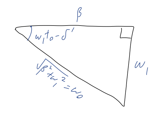
from which we can immediately see that \cos (\omega_1 t_0 - \delta') = \frac{\beta}{\omega_0} and so the other boundary condition equation gives us 0 = A' e^{-\beta t_0} \frac{\beta}{\omega_0} + \frac{F_0}{m \omega_0^2} \\ A' = -\frac{F_0}{m \beta \omega_0} e^{\beta t_0} So, our general solution in region II looks like x_{II}(t) = \frac{F_0}{m \omega_0^2} \left[ 1 - \frac{\omega_0}{\beta} e^{-\beta(t-t_0)} \cos (\omega_1 t - \delta') \right]. If there was no region III, i.e. if the force just switched on and stayed on at t_0, we see that at long times the second term dies off, and we’re just left with the first term, which is exactly the simple solution in the presence of a constant force. Now, let’s confront the last boundary. In region III, after t=t_0 + \tau, the force is gone once again and we have simply the underdamped solution, x_{III}(t) = A'' e^{-\beta t} \cos(\omega_1 t - \delta''). Matching solutions between regions II and III, we must have x_{II}(t_0 + \tau) = x_{III}(t_0 + \tau) \\ \dot{x}_{II}(t_0 + \tau) = \dot{x}_{III}(t_0 + \tau). If we just try to plug in directly, we’ll get a really messy pair of equations to deal with! In fact, it’s not really worth solving the fully general case here. Instead, we can make a simplifying assumption: let’s suppose that \tau is very short compared to the other timescales in the problem, i.e. assume that \beta \tau \ll 1 and \omega_1 \tau \ll 1. In other words, we assume that the force is applied for a very brief window of time. We can then series expand at small \tau to simplify our equations greatly.
This will still lead to some very messy algebra, which I’ll skip past; you know how to set it up at this point. If we slog through it all, we will find a relatively simple final result: x_{III}(t) \approx \frac{F_0 \tau}{m \omega_1} e^{-\beta(t-t_0)} \sin (\omega_1 (t-t_0)). for t > t_0. We might have guessed at the qualitative behavior: if we hit a damped oscillator, it will “ring” and start to oscillate, but the oscillations will die off quickly because of the damping.
5.7.1 The Fourier transform
You might notice that all of this was much more complicated than our Fourier series approach for periodic forces. Unfortunately, the impulse force isn’t periodic, so there’s no way we can use our Fourier series technique - it only happens once. But what if there was a way we could use the Fourier series anyway?
Consider the following periodic force, which resembles a repeated impulse force:
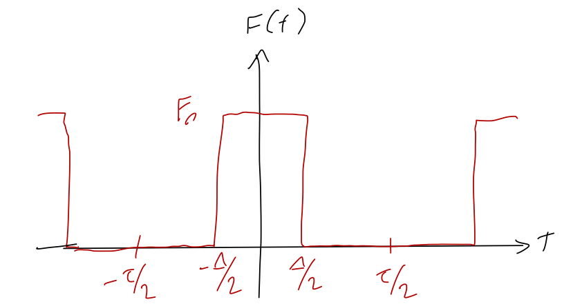
Within the repeating interval from -\tau/2 to \tau/2, we have a much shorter interval of constant force extending from -\Delta/2 to \Delta/2. It’s straightforward to find the Fourier series for this force, but we don’t have to because Taylor already worked it out as his example 5.4; the result is a_0 = \frac{F_0 \Delta}{\tau}, \\ a_n = \frac{2F_0}{n\pi} \sin \left( \frac{\pi n \Delta}{\tau} \right), and all of the b_n coefficients are zero by symmetry, since the force is even.
Now, to apply this to the single impulse, we want to take the limit where \tau \gg \Delta. This is straightforward to do in the Fourier coefficients themselves: we have a_n \approx \frac{2F_0 \Delta}{\tau}. But now we run into a problem when we try to actually use the Fourier series, which takes the approximate form F(t) \approx \frac{F_0 \Delta}{\tau} \left[1 + 2 \sum_{n=1}^\infty \cos \left( \frac{2\pi n t}{\tau} \right) \right]. The problem is that the usual factor of 1/n cancelled out, so the size of our terms is not dying off as n increases. So our usual approach of truncation won’t be useful at all!
There’s something else that is happening at the same time as we try to take \tau \rightarrow \infty, which is equivalent to \omega \rightarrow 0. Remember that we’re summing up distinct Fourier components with frequency \omega, 2\omega, 3\omega... But as \omega goes to zero, these frequencies are getting closer and closer together - and our sum is getting closer and closer to resembling a continuous integral!
This suggests that we try to replace the sum with an integral. We want to think carefully about the limit that \tau \rightarrow \infty. Let’s define the quantity \omega_n = \frac{2\pi n}{\tau}. As \tau becomes larger and larger, the interval between \omega_n is becoming smaller and smaller, to the point that we can imagine it becoming an infinitesmal: d\omega = \frac{2\pi}{\tau} \Delta n where (\Delta n) = 1 by definition, since we sum over integers, but it will be useful notation for what comes next. Let’s take this and rewrite the Fourier sum slightly: F(t) = \sum_{n=0}^\infty (\tau a_n) \cos \left( \omega_n t \right) \frac{\Delta n}{\tau} All I’ve done is multiplied by 1 twice: first to introduce \Delta n, which is 1, and second to multiply and divide by \tau. But the key is that this is now a sum over a bunch of steps which are infinitesmally small, so as \tau \rightarrow \infty, this is a proper Riemann sum and it becomes an integral. Using \Delta n / \tau = d\omega / (2\pi), we can write it as an integral over \omega: F(t) = \frac{1}{2\pi} \int_0^\infty G(\omega) \cos(\omega t) d\omega. The function G(\omega) comes from the Fourier coefficients, specifically from the product \tau a_n:
G(\omega) = \lim_{\tau \rightarrow \infty} \tau \left( \frac{2}{\tau} \int_{-\tau/2}^{\tau/2} f(t) \cos \left( \omega t \right) dt \right) \\ = 2 \int_{-\infty}^\infty f(t) \cos(\omega t) dt.
The function G(\omega) is known as the Fourier transform of F(t). Once again, just like the Fourier series, this is a representation of the function. In this case, there’s no questions about infinite series or truncation; we’re trading one function F(t) for another function G(\omega). There is also no restriction about periodicity - we can use the Fourier transform for any function at all, periodic or not.
One note: there are several equivalent but slightly different-looking ways to define the Fourier transform! One simple difference to watch out for is where the factor of 2\pi goes - it can be partly or totally moved into the definition of G(\omega) instead of being kept in F(t). More importantly, the cosine version that we’re using is actually not as commonly used, in part because it can only work on functions that are even; in general we need both sine and cosine. A more common definition of the Fourier transform is in terms of complex exponentials: F(t) = \int_{-\infty}^\infty G(\omega) e^{i\omega t} d\omega \\ G(\omega) = \frac{1}{2\pi} \int_{-\infty}^\infty F(t) e^{-i\omega t} dt.
Notice that in this case, unlike the Fourier series, there’s a certain symmetry to the definitions of F(t) and G(\omega). This is because both representations are functions here, instead of trying to match a function onto a sum. But the symmetry of the definitions suggests that it should be just as good to go backwards, thinking of F(t) as a representation obtained from G(\omega).
5.7.2 The Dirac delta function
To understand inverting the Fourier transform, we can take these formulas and plug them in to each other. Let’s use the complex exponential version: G(\omega) = \frac{1}{2\pi} \int_{-\infty}^\infty \left( \int_{-\infty}^\infty G(\alpha) e^{i\alpha t} d\alpha \right) e^{-i \omega t} dt (notice that I can’t use \omega twice. In the definition of F(t), \omega is a dummy variable; we’re integrating over it, so I can call it anything I want.) Now, I can do some rearranging of these integrals: G(\omega) = \int_{-\infty}^\infty G(\alpha) \left[ \frac{1}{2\pi} \int_{-\infty}^\infty e^{i(\alpha-\omega)t} dt \right] d\alpha Notice what is going on here; we have the same function G on both sides of the equation, but on the left it’s at a single frequency \omega, while on the right it’s integrated over all possible frequencies. This is sort of familiar, actually; it resembles the orthogonality relation we had for the cosines and sines in the Fourier series, where the integral would be zero except for the special case where the two cosines match in frequency.
In line with the idea of orthogonality, the only way this equation can be true for all \omega and all G is if the object in square brackets is picking out only \alpha = \omega from under the integral, and discarding everything else! In other words, if we define \delta(\alpha - \omega) \equiv \frac{1}{2\pi} \int_{-\infty}^\infty e^{i(\alpha - \omega) t} dt, known as the Dirac delta function (although technically it’s not a function - more on that shortly), then it has the property that \int_{-\infty}^\infty dx f(x) \delta(x-a) = f(a).
The delta function resembles the Kronecker delta symbol, in that it “picks out” a certain value of x from an integral, which is what the Kronecker delta does to a sum. Note that we can put in any function we want, so if we use f(x) = 1, we get the identity \int_{-\infty}^\infty dx \delta(x) = 1. In other words, if we think of \delta(x) as a function on its own, the “area under the curve” is equal to 1. At the same time, we know that it is picking off a very specific value of x from any given function. Combining these two properties, if we try to plot \delta(x), it must look something like this:
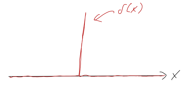
or defining it as a “function”, \delta(x) = \begin{cases} \infty, & x = 0; \\ 0, & x \neq 0. \end{cases} such that the integral over \delta(x) gives 1, as we found above. Once again, this isn’t technically a function, so it’s a little dangerous to try to interpret it unless it’s safely inside of an integral. (If you’re worried about mathematical rigor, it is possible to define the delta function as a limit of a regular function, for example a Gaussian curve, as its width goes to zero.)
From the plot, we can visually observe that it’s important that the delta function spike is located within the integration limits, or else we won’t pick it up and will just end up with zero. In other words, \int_{-1}^3 dx\ \delta(x-1) = 1 but \int_{-1}^3 dx\ \delta(x-4) = 0.
There are some other useful properties of the delta function that we could derive (you can look them up in a number of math references, including on Wikipedia or Mathworld.) Let’s prove a simple one, to get used to delta-function manipulations a bit. What is \delta(kt), where k is a constant real number? As always, to make sense of this we really need to put it under an integral:
\int_{-\infty}^\infty f(t) \delta(kt) dt = ? We can do a simple u-substitution to rewrite: (...) = \int_{t=-\infty}^{t=\infty} f\left(\frac{u}{k} \right) \delta(u) \frac{du}{k} \\ = \frac{1}{k} \int_{-\infty}^\infty f\left( \frac{u}{k} \right) \delta(u) du assuming k>0 for the moment; we’ll come back to the possibility of negative k shortly. Now, the fact that the argument of f has a 1/k in it doesn’t matter, because when we do the integral we pick off f(0): (...) = \frac{f(0)}{k} = \int_{-\infty}^\infty f(t) \left[ \frac{1}{k} \delta(t) \right] dt. Now compare what we started with and what we ended with, and we get \delta(kt) = \delta(t)/k. Again, if k<0 we get an extra sign flip, which would give us a minus sign - but -k if k is negative is just |k|. So we have the full result \delta(kt) = \frac{1}{|k|} \delta(t).
What is the result of the integral
\int_{-\infty}^\infty x^2 \delta(2-x) dx = ?
Answer:
The careful way to do this is once again a u-substitution. If we let u = 2-x, then du = -dx and we have \int_{-\infty}^\infty x^2 \delta(2-x) dx = \int_{+\infty}^{-\infty} (2-u)^2 \delta(u) (-du) being careful to plug in u instead of x for the limits of integration, which flips their signs. The \delta(u) will set u=0, leaving us with (...) = 2^2 = 4, positive since the minus sign in -du cancels the extra minus sign from flipping the limits of integration back around.
We could have seen this answer coming without going through all the math if we think visually. We know that \delta(x) is always positive, so \delta(2-x) has to actually be the same thing as \delta(x-2), at which point we use the defining identity to just plug in 2^2 = 4. Since \delta(x-2) and x^2 are both positive, we can also easily see that the integral has to be positive, ruling out the negative-sign answers.One more comment on the delta function, bringing us back towards physics. We use the delta function often to represent “point particles”, which we imagine as being concentrated at a single point in space - not totally realistic, but often a useful approximation. In fact, one example where this is realistic is if we want to describe the charge density of a fundamental charge like an electron. Suppose we have an electron sititng on the x-axis at x=2. The one-dimensional charge density describing this would be \lambda(x) = -e \delta(x-2). So the electron has infinite charge density at point x=2, and everywhere else the charge density is zero. This might seem unphysical, but it’s the only consistent way to define density for an object that has finite charge but no finite size. If we ask sensible questions like “what is the total charge”, we get good answers back: Q = \int_{-\infty}^\infty \lambda(x) dx = -e \int_{-\infty}^\infty \delta(x-2) dx = -e which is exactly the answer we expect! One final thing to point out here: if we think about units, 1-d charge density should have units of charge/distance, which means the units of the delta function are inverse to whatever is inside of it. This makes sense, because of the identity \int dt \delta(t) = 1. Since dt has units of time, \delta(t) here has to have units of 1/time.
5.7.3 Fourier transforms and solving the damped, driven oscillator
Let’s go back to our non-periodic driving force example, the impulse force, and apply the Fourier transform to it. Recall that our function for the force is F(t) = \begin{cases} F_0, & t_0 \leq t < t_0 + \tau, \\ 0, & {\textrm{elsewhere}} \end{cases} The Fourier transform of this function is very straightforward to find. Since this isn’t even around t=0, let’s use the most general complex exponential form: G(\omega) = \frac{1}{2\pi} \int_{-\infty}^\infty e^{-i\omega t} F(t) dt \\ = \frac{F_0}{2\pi} \int_{t_0}^{t_0 + \tau} e^{-i\omega t} dt \\ = \left. \frac{-F_0}{2\pi i \omega} e^{-i \omega t} \right|_{t_0}^{t_0 + \tau} \\ = -\frac{F_0}{2\pi i \omega} \left[ e^{-i\omega (t_0+\tau)} - e^{-i\omega t_0} \right] \\ = -\frac{F_0}{2\pi i \omega} e^{-i\omega(t_0 + \tau/2)} \left[ e^{-i\omega \tau/2} - e^{i \omega \tau/2} \right] \\ = \frac{F_0}{\pi \omega} e^{-i\omega(t_0 + \tau/2)} \sin (\omega \tau/2).
What good does this do us? Let’s recall the original equation that we’re trying to solve, \ddot{x} + 2\beta \dot{x} + \omega_0^2 x = \frac{F(t)}{m}. Now, although F(t) and G(\omega) are equivalent - they carry equal information about a single function - we can’t just plug in G(\omega) on the right-hand side, because to get that from F(t) we have to do a Fourier transform, i.e. take an integral over t. That means we have to Fourier transform both sides of the equation. Let’s define the Fourier transform of x as well, \tilde{x}(\alpha) = \frac{1}{2\pi} \int_{-\infty}^\infty x(t) e^{-i\alpha t} dt What happens if I have derivatives of x(t) under the integral sign? We can use integration by parts to move the integral over, and it’s not difficult to prove the general result \tilde{x^{(n)}}(\alpha) = (i \alpha)^n \tilde{x}(\alpha), i.e. the Fourier transform of a time derivative of x(t) is just i\alpha times the Fourier transform of the original. Now we know enough to take the Fourier transform of both sides above: (-\alpha^2 + 2i \beta \alpha + \omega_0^2) \tilde{x}(\alpha) = \frac{G(\alpha)}{m} (where the same frequency \alpha appears on both sides, since we’re applying the same Fourier transform to both sides!) This is a very powerful result, because there is no differential equation left at all: we can simply write down the answer, \tilde{x}(\alpha) = \frac{G(\alpha)/m}{-\alpha^2 + 2i \beta \alpha + \omega_0^2} and take one more Fourier transform to get the time-domain solution, x(t) = \int_{-\infty}^\infty \tilde{x}(\alpha) e^{i\alpha t} d\alpha = \int_{-\infty}^\infty \frac{G(\alpha)/m}{-\alpha^2 + 2i \beta \alpha + \omega_0^2} e^{i\alpha t} d\alpha. This is a powerful and general way to deal with certain linear, non-homogeneous ODEs - you can see immediately that this will extend really nicely even to higher than second order, since we still get a simple algebraic equation! This method is sometimes referred to as “solving in frequency space”, because we transform from considering time to frequency using the Fourier transform and the equation simplifies drastically.
The bad news is that even for a relatively simple driving force like our impulse, this integral is a nightmare to actually work out! Evaluating difficult integrals like this, particularly ones where complex numbers are already involved, is a job for the branch of mathematics known as complex analysis. Such methods can be combined with another method called the method of Green’s functions, which uses the delta function to allow us to do the difficult integral just once, and end up with simpler integrals to describe solutions with more complicated driving forces. Both of these powerful methods are beyond the scope of this class, but they are widely used and important in many physics systems, so you will likely encounter them sooner or later in other physics or engineering classes!