4 Energy and work
Our next big physics topic will be energy. Energy also satisfies a conservation law, like momentum and angular momentum. However, energy is much more subtle; as Taylor points out, a lot of confusion tends to come from the fact that energy comes in many different forms, whereas there’s only one kind of (linear or angular) momentum. This will also lead us naturally into our next big math topic, which is vector calculus.
4.1 Work and kinetic energy
Since this is a mechanics class, we’ll start with kinetic energy, which is energy associated with motion. For a point mass, the kinetic energy T is given by the formula T = \frac{1}{2} mv^2.
You’ll notice right away that like linear momentum, energy is not independent of our choice of coordinates; if I choose a moving coordinate system, then v will change and so will T. So in and of itself, energy is not some immutable property of an object; it’s a useful construct that will help us solve for the motion.
To better understand the physical meaning of energy, let’s try to connect it to Newton’s laws. We start by just taking a time derivative to see what happens. To do this properly, we should be careful and remember that v^2 is really \vec{v} \cdot \vec{v}, so the derivative is: \frac{dT}{dt} = \frac{m}{2} \frac{d}{dt} \left( \vec{v} \cdot \vec{v} \right) \\ = \frac{m}{2} \left( \vec{v} \cdot \dot{\vec{v}} + \dot{\vec{v}} \cdot \vec{v} \right) \\ = m \vec{v} \cdot \dot{\vec{v}} \\ = \frac{d\vec{r}}{dt} \cdot \vec{F}_{\textrm{net}}, using Newton’s second law at the end, and I wrote out the time derivative to make things look more symmetric. So the change in kinetic energy is given by the dot product of applied force with the velocity, which seems interesting but isn’t really enlightening yet.
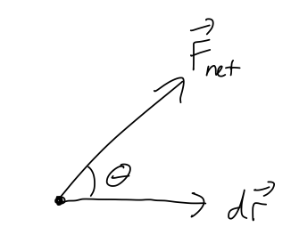
Now suppose that we’re interested in what is happening to our system during an infinitesmal time interval dt. We can multiply both sides by dt to find the equation dT = \vec{F}_{\textrm{net}} \cdot d\vec{r} \equiv dW_{\textrm{net}} where the right-hand side defines the infinitesmal work, dW. Let’s make a couple of useful observations about dW before we move on to integrating it, all of which apply to work in general. First of all, notice that dW is a scalar since it comes from a dot product. In fact, we can rewrite it using one of our dot-product identities as dW_{\textrm{net}} = F_{\textrm{net}} dr \cos \theta.
It’s important to emphasize a few special cases that can be counter-intuitive:
- dW_{\textrm{net}} can be zero, even if F_{\textrm{net}} is non-zero. (From above, this happens when \theta = 90^\circ, i.e. when \vec{F}_{\textrm{net}} is perpendicular to dr.)
- dW_{\textrm{net}} can be negative, if F_{\textrm{net}} and d\vec{r} point in opposite directions. (A simple example is a particle which is decelerating, so the net force is opposite its direction of motion.)
If we integrate both sides as our mass moves from point \vec{r}_1 to point \vec{r}_2, then we find the result T_2 - T_1 = \int_{\vec{r}_1}^{\vec{r}_2}\ dW_{\textrm{net}} = \int_{\vec{r}_1}^{\vec{r}_2}\ d\vec{r} \cdot \vec{F}_{\textrm{net}}, or more compactly, if we call the result of the integral over dW_{\textrm{net}} as just W_{\textrm{net}} (the net work), then we find:
The change in kinetic energy of a point mass as it moves from \vec{r}_1 to \vec{r}_2 is equal to the net work done:
\Delta T = W_{\textrm{net}} \equiv \int_{\vec{r}_1}^{\vec{r}_2}\ d\vec{r} \cdot \vec{F}_{\textrm{net}}.
This is an important relationship, because it gives us a way to interpret what kinetic energy actually means physically.
First, a brief comment on my notation above. It’s important to emphasize that the work-KE theorem is only true for a single point mass, and that it’s only true if we use the net force. However, it’s often useful to define the work done by a single force, which we can do using the same equation, W = \int_{\vec{r}_1}^{\vec{r}_2} d\vec{r} \cdot \vec{F}. Since d\vec{r} \cdot \vec{F}_{\textrm{net}} splits apart into d\vec{r} \cdot \vec{F}_1+ d\vec{r} \cdot \vec{F}_2 + ... in the case of multiple forces, the work also splits apart neatly, W_{\textrm{net}} = W_1 + W_2 + ....
Before we get to solving specific problems, the “big picture” we can see from the work-KE theorem is that changes in kinetic energy tell us something about the overall motion of a physical object. Although we can calculate T for an object at any moment in time, the significance of T is that it summarizes the history of how our object has moved. If our object starts from rest, the value of T later on is related to the sum total of all of the net forces acting in the direction of its path.
We’ll get to how to deal with the integral shortly, but there’s a specific case where it’s easy to simplify. If the net force is constant, then W = \vec{F}_{\textrm{const}} \cdot \int_{x_1}^{x_2} dx = \vec{F}_{\textrm{const}}\ \cdot \Delta \vec{x} which will be useful for considering some simple examples.
Here, you should complete Tutorial 4A on “Work-KE theorem”. (Tutorials are not included with these lecture notes; if you’re in the class, you will find them on Canvas.)
You drop your phone (mass m = 200 g) on the floor, from a height of 1m and from rest; fortunately, it’s in a protective case so it isn’t broken! But you notice a 0.5mm dent left in the case. Assuming that the floor provided a constant force F to stop your phone’s fall, how large is F in Newtons?
Answer:
First, we want to know how fast the phone is moving when it gets to the ground, which is a simple kinematic formula: first, the time to hit the ground is h = \frac{1}{2} gt_f^2 \Rightarrow t = \sqrt{\frac{2h}{g}} = 0.45\ \textrm{s} and then the speed at this time is v_f = v(t_f) = gt_f = 4.4\ \textrm{m}/\textrm{s}.
Now we’re almost done, since the last step is to apply the work-KE theorem. With a constant force, the work is just W = Fd, where d is the stopping distance of 0.5 mm (the size of the dent.) Setting this equal to the change in KE, we have F d = \frac{1}{2} mv_f^2 - 0 \Rightarrow F = \frac{1}{2d} mv_f^2. Plugging in numbers, we have a force of 650 N, which would give an acceleration of about 330 times g - pretty substantial, but not necessarily enough to break the phone, fortunately!
4.1.1 Line integrals
Before we can continue our study of work and kinetic energy, we have to deal with an important question: how do we evaluate the integral for work in general? Having another look at it: W_{\textrm{net}} = \int_{\vec{r}_1}^{\vec{r}_2} \vec{F}_{\textrm{net}} \cdot d\vec{r} How do we interpret this integral, where the integration variable is a vector? The best way to understand what this expression means is to go back to the infinitesmal picture for dW, and imagine building up the whole integral by just stringing together infinitesmal pieces:
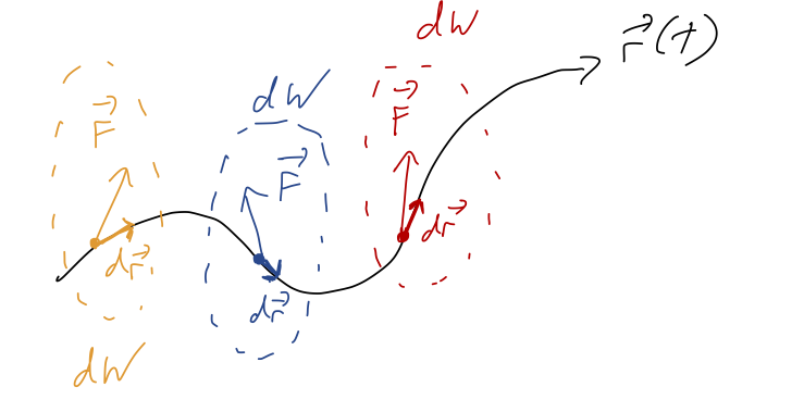
So the integral for W is a sum along the path traced out by \vec{r}., W = \sum_i dW_i \rightarrow \int dW
where the sum becomes an integral as we make our steps along the trajectory d\vec{r} smaller and smaller. Notice that this is not the “area under the curve” or anything related to it; we’re summing up the dot products \vec{F}_{\textrm{net}} \cdot d\vec{r} as we follow the curve. This is an example of a line integral.
There’s one special case where we already know how to do the integral: if the motion is one-dimensional. For one-dimensional motion, all vectors have only one component, so the dot product is trivial. If we call our single direction x, then W_{1d} = \int_{x_1}^{x_2} \vec{F}_{\textrm{net}}(x) \cdot d\vec{x} (I’m keeping the dot product notation to remind us that the directions still matter in one dimension, so we can get minus signs here.)
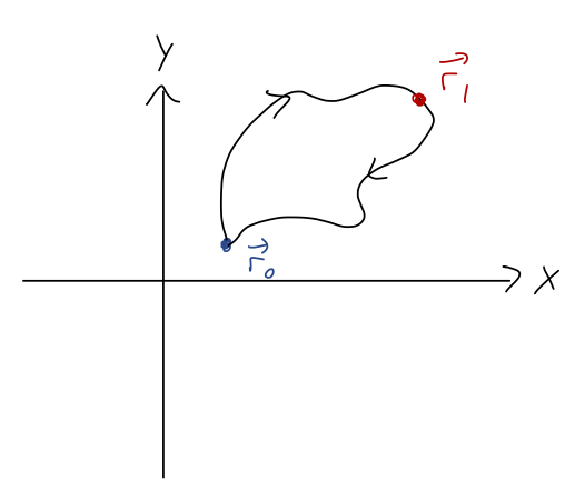
Now let’s pick a concrete example in two dimensions to see how things get tricky. Suppose that we have a constant force of the form \vec{F} = Fx\hat{x} + 2F\hat{y}, and we’d like to compute the work from \vec{r}_1 = (0,0) to \vec{r}_2 = (2,1).
First question: how do we interpret the vector differential d\vec{r}? We already know that derivatives of vectors are simple to evaluate: we just take the derivative of each component. Similarly, d\vec{r} just means we have a differential length in each component. In Cartesian coordinates, d\vec{r} = dx \hat{x} + dy \hat{y} + dz \hat{z}. So in our example, we can evaluate the dot product to find W = \int_{\vec{r}_1}^{\vec{r}_2} (Fx dx + 2F dy). The appearance of two differentials at once, dx and dy, signals that we can’t just evaluate this integral normally yet. More importantly, we have to specify one more thing not written down, which is the path along which we want to evaluate this integral. This is one of the sloppy things about this notation, although it’s used commonly: there are infinitely many ways to get from \vec{r}_1 to \vec{r}_2!
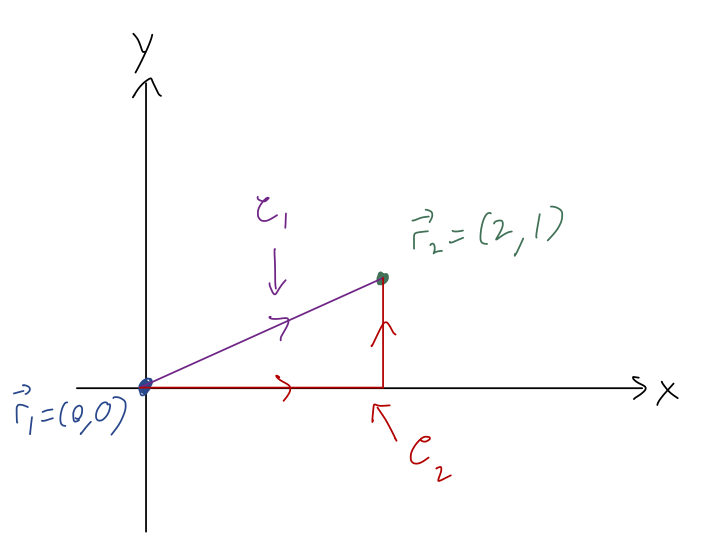
When we do a line integral, we’re actually choosing a directed path, hence the arrows on the sketch above, which tell us where we start and where we end. Just like a regular integral, if we go backwards (reverse the limits of integration so we move from \vec{r}_2 to \vec{r}_1), then we get an extra minus sign.
In math books, the integral will often be written instead as W = \int_{\mathcal{C}} \vec{F} \cdot d\vec{r}, where \mathcal{C} denotes a curve - the entire path we take, along with its endpoints. In physics applications, when we do the work integral, the curve is often just \vec{r}(t), the trajectory followed by our point mass.
Let’s pick one of the curves above and try to evaluate the integral. I’ll start with the straight line path, \mathcal{C}_1. If we think about it for a moment, the way a path is mathematically defined is an equation relating our coordinates to each other. In this case, we can write simply y = \frac{1}{2}x along \mathcal{C}_1. This relationship is true as long as we follow the curve. But we can use this to collapse our two differentials together: we have dx = 2dy so we can rewrite the line integral as W_1 = \int_{\mathcal{C}_1} (F xdx + 2F dy) \\ = \int_0^1 (F (2y) (2 dy) + 2F dy) \\ = F \left( \left. 4 \frac{y^2}{2} \right|_0^1 + \left. 2y \right|_0^1 \right) \\ = 4F.
This shows the basic idea of evaluating a line integral: although it looks like it has multiple coordinate differentials in it, when we move along a specific line, we can relate our coordinates together and collapse down to a single differential. Then we just have a normal integral to do! (It will always be a single integral, because a line is one-dimensional; we can always describe the distance along a line using a single number, whether the line is curved or not.)
An important feature of this method is that the way in which we collapse our multiple coordinates down to one is not unique. For example, we could have replaced dy instead of dx, and we’ll get the same answer: W_1 = \int_{\mathcal{C}_1} (Fx dx + 2F (dx/2)) \\ = \int_0^2\ F(1+x) dx \\ = F \left. x \right|_0^2 + F \left. \frac{1}{2} x^2 \right|_0^2 \\ = 4F. We don’t even have to stick to x and y! Another way to describe \mathcal{C}_1 is using a parametric equation: if we call our parameter s, then x(s) = 2s \\ y(s) = s \\ also defines the line y=x/2; try plugging in x(s) and y(s) to the line equation if it’s not obvious! Looking at the endpoints, we start at s=0 and end at s=1. Now we replace both coordinates, using dx = 2ds and dy = ds: W_1 = \int_{\mathcal{C}_1} (F (2s) (2 ds) + 2F ds) \\ = \int_0^1\ 2F (2s+1) ds = 4F.
Any line integral is always, implicitly, an integral against some single parameter s that describes the curve \mathcal{C} we are integrating along. Sometimes, it’s convenient to use coordinates like x or y as the parameter s, but we don’t have to. Pick whatever s is most convenient for a given curve!
Here’s yet another parameterization of the same curve: x(u) = 1-u\\ y(u) = (1-u)/2 where u runs from +1 to -1. Verify that this gives the same answer as above!
Answer:
First, we have to convert the differentials: from above we see dx = -du and dy = -du/2. Then we can plug in to the integral:
W_1 = \int_{\mathcal{C}_1} (F (1-u) (-du) + 2F (-du/2)) \\ = \int_{+1}^{-1} du\ F (-1 + u - 1) \\ = \left. F (-2u + \frac{1}{2}u^2) \right|_{+1}^{-1} = 4F.
No matter how we parameterize the curve, the result will always be the same - we’re not changing anything except how we choose to describe it. Finding a good parameterization can be kind of an art (like choosing a good set of coordinates!) In physics applications, time itself is often a good parameter to describe the path - we’re already used to solving for the motion \vec{r}(t)!
Now let’s consider the second curve \mathcal{C}_2. This is, in general, a different integral - even though the endpoints are the same, the path is different! This path isn’t a smooth curve - it has a sharp corner where the path suddenly changes. This means that we should do the integral piecewise, meaning that we divide up the path into smooth parts and deal with them one at a time. Here, the pieces of the path are very simple: from the origin, we have the curve y = 0 (which also implies dy = 0). For the second path of the curve, we have the fixed value x=2 - since this is constant, we see also that dx = 0. Thus, we can write the work integral along \mathcal{C}_2 as: W_2 = \int_{\mathcal{C}_2} (F x dx + 2F dy) \\ = \int_0^2 F x dx + \int_0^1 2F dy \\ = 2F + 2F = 4F.
In this particular case, we got the same answer again! In fact, this is not just a coincidence: you will get 4F for any path from (0,0) to (2,1) and this particular force. There is a deeper reason for this that we will see soon - but keep in mind, this is NOT guaranteed to be true for any force, so don’t just assume you can pick any path for an arbitrary force!
By the way, it’s often useful to visualize what’s going on in these line integrals before we just do the math out. Sketching the paths is only half of the visualization, because the direction and size of the force also matters. However, while the path is just a single line through space, the force \vec{F} is generally defined everywhere in space. As a result, we visualize it by drawing a force field plot. (A vector field is just a set of vectors that exist everywhere in space, whose values and directions are functions of position.)

This makes it simpler to understand the work resulting from certain paths. In particular, if we move perpendicular to the force field, then \vec{F} \cdot d\vec{r} is always zero and the work will be zero. For path \mathcal{C}_1 (or \mathcal{C}_2 as well), we can easily predict from the force field plot that the work will be positive, since we are generally moving in the same direction that the force points (so \vec{F} \cdot d\vec{r} > 0.)
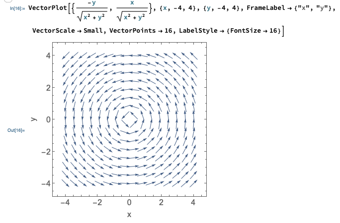
Since it’s often useful to sketch vector fields, it’s worth knowing that Mathematica has a function to do it for us, the VectorPlot[] function. Here’s an example:
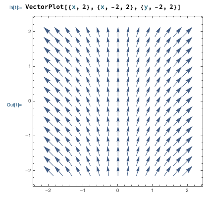
In Mathematica, vectors are denoted using curly braces {,}. You can see the input notation for VectorPlot above: the first argument is the vector field as a function, i.e. we enter {F_x, F_y} = {x, 2} for the vector field we’ve been working with. The last two arguments define the variable names and range to plot over, first x and then y.
Here, you should complete Tutorial 4B on “Line integrals”. (Tutorials are not included with these lecture notes; if you’re in the class, you will find them on Canvas.)
4.1.2 Line integrals and curvilinear coordinates
There are certain forces and/or certain paths for which the other coordinate systems we introduced this semester (cylindrical and spherical) will make things a lot simpler. For paths, working in different coordinates just gives us to a different way to parametrize the path - if we have a circular path, for example, then polar coordinates might be helpful. But as we’ve seen, there are usually multiple ways to choose the parameter s for any given path.
On the other hand, curvilinear vector coordinates can be very powerful for simplying line integrals whenever the force is most easily written using cylindrical or spherical components. To see this, let’s do another example. Suppose we have a force which is proportional to the polar unit vector \hat{\phi}, \vec{F} = F\hat{\phi} and we’re interested in the work done along a counterclockwise half-circle path from (1,0) to (-1,0).
Sketching vector fields makes my hand hurt, so here’s another Mathematica plot:
(I converted from polar to Cartesian for the plot - more on that below.) Think about it - does this match what you expected the plot to look like?
Next, we need d\vec{r} so we can find the dot product. Since we have \vec{F} in polar coordinates, we should use d\vec{r} in the same coordinates. We’ll assume z=0, but in full 3-d cylindrical coordinates, we know that \vec{r} = \rho \hat{\rho} + z \hat{z} To find d\vec{r}, one way would just be to start with the Cartesian version d\vec{r} = dx\ \hat{x} + dy\ \hat{y} + dz\ \hat{z} and apply our coordinate change. More directly, we can just calculate the derivative of \vec{r} with respect to some parameter, like t, and then cancel off the dt’s. Let’s try it that way: \frac{d\vec{r}}{dt} = \dot{\rho} \hat{\rho} + \rho \frac{d\hat{\rho}}{dt} + \dot{z} \hat{z} \\ = \frac{d\rho}{dt} \hat{\rho} + \rho \frac{d\phi}{dt} \hat{\phi} + \frac{dz}{dt} \hat{z} using the result for d\hat{\rho}/dt that we worked out back at the start of the semester. Cancelling off the dt’s, d\vec{r} = d\rho\ \hat{\rho} + \rho d\phi\ \hat{\phi} + dz\ \hat{z}. In case you ever need it, I’ll save you some trouble and give you the result for spherical coordinates: d\vec{r} = dr\ \hat{r} + r d\theta\ \hat{\theta} + r\sin \theta d\phi\ \hat{\phi}.
Using our result, we have the simple result dW = \vec{F} \cdot d\vec{r} = F \rho d\phi
Next, we parameterize the half-circular path. Any time we have a path like a circle or a spiral, an angle is a natural parameter to use. In fact, since this is just a section of the unit circle, we can easily write the path in the trivial-looking form \rho = 1, \\ \phi = \phi, starting at \phi=0 and ending at \phi=\pi. Thus, the integral can be written simply as W = \int_0^\pi F d\phi = \pi F. (Don’t be confused by units! Remember, our path has units of distance, so this is something like “pi meters times the constant force F.”)
Note that the length of the path can also be found by a line integral, which amounts to adding up a bunch of infinitesmal length segments: \ell = \int |d\vec{r}| = \int \sqrt{d\vec{r} \cdot d\vec{r}} = \int \sqrt{\rho^2 d\phi^2} = \int_0^\pi \rho\ d\phi = \pi (this is also easy to find geometrically as just half the circumference of a circle, of course.) So in this case, just like in our one-dimensional examples, we have simply W = F \ell. This happens because for this particular path and force, \vec{F} and d\vec{r} point in the same direction as one another along the entire path.
In this problem it was sort of obvious to choose polar coordinates, because of how we were given the force. But we could have been given \vec{F} in Cartesian coordinates instead: \vec{F} = -\frac{y}{\sqrt{x^2 + y^2}} \hat{x} + \frac{x}{\sqrt{x^2 + y^2}} \hat{y} You might be able to spot the fact that this is just \hat{\phi} from the expression, but a more reliable way to see that polar coordinates might be the way to go would be to plot the force field (this is one reason plotting vector fields is useful!) If you didn’t spot it, your integrals would be a lot more painful…
Another important note on coordinate dependence: it’s generally a better idea to let the force field dictate the coordinate choice, rather than the path. For example, suppose we had this same circular force, but the straight-line path y = x/2 from our previous example. It’s actually not so hard to parametrize that path in polar coordinates: remembering how polar and Cartesian are related, the line equation above becomes \rho \sin \phi = \frac{1}{2} \rho \cos \phi \Rightarrow \tan \phi = \frac{1}{2}. So this is a path with constant \phi and constant z, giving d\vec{r} = d\rho \hat{\rho}. We don’t have to go any further, since \vec{F} \cdot d\vec{r} = 0 and the work is just zero. (It will still be zero in Cartesian coordinates, but the integral will be much more work!)
That was too easy, since a straight line through the origin is just in the \hat{\rho} direction and therefore still nice in cylindrical coordinates. What about this path, the fixed vertical line x=1 from (1,1) to (1,-1)?
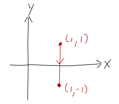
The equation for this line in polar coordinates is x = 1, which is just \rho = 1 / \cos \phi. This path changes in both \rho and \phi, so in general we will pick up both; but for the force we’re considering \vec{F} = F \hat{\phi}, the dot product is still \vec{F} \cdot d\vec{r} = \rho d\phi. Thus, the work integral still takes the same form we found above, W = \int \vec{F} \cdot d\vec{r} = \int F \rho d\phi \\ = F \int_{\pi/4}^{-\pi/4} \frac{d\phi}{\cos \phi} \\ \approx (-1.76\ {\textrm{m}}) F where I used Mathematica to do the integral numerically - it ends up being a complicated combination of logs and trig functions. I’m just reading the \phi limits of integration off the plot geometrically, but in general we get them by solving the equation of our line at the given points.
Here’s a more interesting line, y = 1 + x/2 from (0,1) to (2,2):
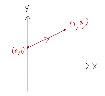
What is the line integral \int_{\mathcal{C}} \vec{F} \cdot d\vec{r} over this curve, for the force \vec{F} = F\hat{\phi}?
Answer:
If we substitute in the coordinate conversions for both x and y in polar, the equation for the line becomes: \rho \sin \phi = 1 + \frac{1}{2} \rho \cos \phi \\ \rho (2\sin \phi - \cos \phi) = 2 \\ \rho(\phi) = \frac{2}{2\sin \phi - \cos \phi}. How about the endpoints? At (0,1) we obviously have \phi = \pi/2; plugging this in to our \rho(\phi) is a good check of our work, and it gives \rho(\pi/2) = \frac{2}{2 - 0} = 1 which is correct. The other endpoint is at \phi = \pi/4, so our line integral is (using \vec{F} \cdot d\vec{r} = F \rho d\phi from above): W = \int_{\pi/2}^{\pi/4} d\phi \frac{2}{2\sin \phi - \cos \phi} d\phi I wouldn’t want to do this integral by hand, although it does have a closed-form answer in terms of \tan and \tanh. Doing it numerically, I find W \approx (-1.2\ \textrm{m}) F.The moral of these examples is that the force is the most important factor in your choice of coordinate system for a line integral, because we have to deal with the vector components of the force. Once that’s out of the way, it’s easy to make our path conform to whatever coordinates we’ve chosen.
To recap, when faced with a line integral, we need to work through the following steps to find the answer:
- Choose vector coordinates and find \vec{F} \cdot d\vec{r}. (The form of \vec{F} is usually most important in coordinate choice, but don’t ignore the path completely.)
- Parameterize the path, writing it in terms of a single coordinate or parameter.
- Use the results of 1) and 2) to write the work integral as a regular integral over our single parameter.
- Do the integral and find the answer!
If you feel like you need more line integral practice, here’s one more exercise you can try.
Calculate the work integral W = \vec{F} \cdot d\vec{r} for the force \vec{F} = 2\vec{r} and parabolic path x = 1-y^2, from (1,0) to (0,1).
Answer:
Let’s start by sketching the path:
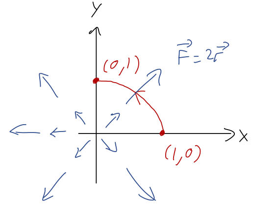
It might be tempting to choose polar coordinates since the force field is radial, but radial force is pretty easy to describe in Cartesian coordinates too, and our path will be easier in Cartesian. (If we had a force in the \hat{\phi} direction, we’d almost certainly want polar instead!) Using Cartesian, we have \vec{F} = 2x \hat{x} + 2y \hat{y} and so \vec{F} \cdot d\vec{r} = 2Fx dx + 2Fy dy.
Next, we parameterize the path. Here y itself is a nice parameter, since we already have the path written in the form x = 1-y^2. In terms of differentials, we have dx = -2y dy and in terms of y, our path begins at y=1 and ends at y=0. So writing out our line integral, W = \int \vec{F} \cdot d\vec{r} = \int (2Fx dx + 2Fy dy) \\ = 2F \int_1^0 (1-y^2) (-2y dy) + y dy \\ = 2F \int_1^0 dy\ (-y + 2y^3) \\ = 2F \left. \left(-\frac{y^2}{2} + \frac{y^4}{2} \right) \right|_0^1 \\ = 0.
Although the work is exactly zero here, it’s sort of a coincidence: we notice that the cancellation of y^2 and y^4 only worked at y=0 and y=1, so pretty much any other starting or ending points along this curve would yield non-zero work.
4.2 Potential energy
Now that we know how to calculate line integrals, let’s go back to the physical meaning of work. In mechanics, we aren’t going to be dealing with completely arbitrary paths; the work-KE theorem only applies to the path which results from Newton’s laws and whatever forces are applied.
At the beginning of this section, I mentioned that energy comes in many forms. To really see how work and energy can be useful, we need to introduce a second form of energy, which is called potential energy. You may remember the buzzwords from intro physics: a potential energy can only be defined for a conservative force. This turns out to be a consequence of how we define a conservative force, acting on a point mass:
- Conservative forces depend only on \vec{r} and constants.
- The work done by a conservative force from \vec{r}_1 to \vec{r}_2 is independent of the path taken.
When both of these properties are satisfied, if we’re given two points anywhere in space, we immediately know the work done by the conservative force when we move from one to the other. (Property 1 matters because we don’t need any extra info to decide the work done, like how long it took to move between the points or how fast the object was moving.)
Now let’s pick a special point \vec{r}_0 somewhere in space and hold it fixed. The work done to get to any other point \vec{r} from this special point is a function only of where the second point is: W_{\vec{r}_0 \rightarrow \vec{r}} = \int_{\vec{r}_0}^{\vec{r}} \vec{F} \cdot d\vec{r} = -U(\vec{r}) This defines the potential energy function. (It only depends on \vec{r}, because we’ve agreed to hold \vec{r}_0 fixed.) The minus sign I added at the end is extremely important, as we’ll see below! Basically, it has to do with energy conservation: positive work will give a positive change in kinetic energy, which will be compensated by a negative change in potential energy so the total stays fixed.
Now, let’s do a short mathematical proof that will let us make two nice observations. If we try to calculate U(\vec{r}_0), we find the following: U(\vec{r}_0) = -\int_{\vec{r}_0}^{\vec{r}_0} \vec{F} \cdot d\vec{r} \\ = -\int_{\vec{r}_0}^{\vec{r}_1} \vec{F} \cdot d\vec{r} - \int_{\vec{r}_1}^{\vec{r}_0} \vec{F} \cdot d\vec{r} where I’m now just picking another arbitrary point \vec{r}_1 and using the properties of definite integration to split it up. Okay, this isn’t a normal integral. Really, the original line integral represents a closed path from \vec{r}_0 back to itself, and I’ve picked a point somewhere along that path and divided it in half:
Reversing the limits of any integral, including a line integral, just gives us a minus sign: U(\vec{r}_0) = -\int_{\vec{r}_0}^{\vec{r}_1} \vec{F} \cdot d\vec{r} + \int_{\vec{r}_0}^{\vec{r}_1} \vec{F} \cdot d\vec{r} = 0. These two integrals are on two different curves, but since \vec{F} is conservative it doesn’t matter; their results are equal and they cancel. The first nice observation is that picking a reference point is the same thing as choosing where our potential energy function is equal to zero, which you’ll remember as something you can do with e.g. the gravitational potential.
If you choose a different reference point \vec{r}'_0, then your potential energy function will be different, but in a simple way: U'(\vec{r}) = -\int_{\vec{r}'_0}^{\vec{r}} dW = -\int_{\vec{r}'_0}^{\vec{r}_0} dW - \int_{\vec{r}_0}^{\vec{r}} dW \\ = U(\vec{r}_0') - U(\vec{r}) or in other words, the difference between U and U' is just a shift by a constant.
The second nice observation we can make is that we’ve just showed that for any force which satisfies property 2 above (work done is path-independent), the work done around a closed path is exactly zero. You may remember the special notation for closed-path integrals from vector calculus: \oint \vec{F} \cdot d\vec{r} = 0. If you remember that notation, you probably also remember that \vec{F} \cdot d\vec{r} shows up in a very powerful result called Stokes’ theorem. We’ll come back to that later on: it will give us a much clearer picture of why any particular force should obey property 2 above, which seems sort of arbitrary right now.
Back to our general discussion of potential energy U. Assuming for the moment that the corresponding \vec{F} is the only force acting, the work-KE theorem applies: T(\vec{r}_2) - T(\vec{r}_1) = W_{1 \rightarrow 2} = \int_{\vec{r}_1}^{\vec{r}_2} \vec{F} \cdot d\vec{r} = -U(\vec{r}_2) + U(\vec{r}_1) or rearranging, T(\vec{r}_1) + U(\vec{r}_1) = T(\vec{r}_2) + U(\vec{r}_2). In other words, the combination E = T + U, which we call the mechanical energy (or just “the energy” when we’re doing classical mechanics), doesn’t change as we move from \vec{r}_1 to \vec{r}_2. Since this is true for any two points we choose, and since the path and other variables can’t change the work, we see that in the presence of a conservative force, energy is conserved: \frac{dE}{dt} = 0.
Since we used the work-KE theorem, we technically assumed above that \vec{F} is the only force acting in our system. If we have multiple forces, remember that we can divide net work up into the sum of work due to each individual forces. If they’re all conservative, then we can write a separate potential energy function for each force. So the more general version of the mechanical energy is E = T + U_1 + U_2 + U_3 + ... if we have several forces \vec{F}_1, \vec{F}_2, \vec{F}_3...
Of course, as we just noted there are plenty of non-conservative forces around. The work-KE theorem still applies to them, and we can still split them up. If we have both conservative and non-conservative forces, then \Delta T = W_{\textrm{net}} = W_{\textrm{cons}} + W_{\textrm{non-cons}} \\ = -\Delta U + W_{\textrm{non-cons}} or \Delta E = W_{\textrm{non-cons}} So energy is not conserved if we have non-conservative forces, but we know exactly how it will change if we keep track of the work done by those forces.
Here’s a quick note about the deeper interpretation of this absence of energy conservation, since I commented early that conservation of energy is a really important and general physical principle. Friction and air resistance are not fundamental forces: ultimately, they come from electromagnetic forces between the atoms in our object and the surface or medium providing the force. All of the known fundamental forces of nature are conservative, which means that total energy is conserved, period. When we find a non-zero \Delta E due to something like friction, that “lost” energy is just being transferred into another form - mostly heat, in the case of friction. When multiple conservative forces are present, energy will be exchanged between the different potentials and kinetic energy (see here for a classic example!), but total E is always the same.
One more brief aside, about magnetic fields, which are sort of a weird example. They are non-conservative because they depend on speed, but they also don’t do any work at all because the magnetic force is always perpendicular to \vec{v}! So a system including a magnetic field will still conserve mechanical energy - but we can’t write a potential energy function (of the form we’re using here) to describe the motion. (In other words, conserving energy alone isn’t sufficient for a force to be “conservative” by the definition we’re using.) Normal forces are even weirder, but they fall into the same category as magnetic force: they usually don’t do any work at all, but they’re not technically considered to be conservative and we can’t use potential energy to describe normal forces.
At this point, Taylor does an example of mixing conservative and non-conservative forces, involving a sliding block with friction. We solved the sliding block with friction way back in chapter 1, but work gives a quicker way to find the speed as a function of the height of the block. I’ll skip this example because Taylor already did it, and unfortunately there aren’t any other good simple examples of this sort of thing: you could try to do a similar trick with linear air resistance, but the equations are unsolvable and you have to resort to numerics anyway, so using energy and work doesn’t really help.
Let’s do a concrete example: a charge +q is suspended in a uniform electric field, \vec{E} = E_0 \hat{x}. The force on the charge is proportional to the field \vec{F} = q\vec{E} = qE_0 \hat{x}.
The force due to a (static) electric field is conservative, so we can go ahead and calculate a potential energy function by using the definition: U(\vec{r}) = -\int_{\vec{r}_0}^{\vec{r}} \vec{F} \cdot d\vec{r} = -\int_{\vec{r}_0}^{\vec{r}} qE_0 dx.
Normally, to continue we’d need to pick a reference point \vec{r}_0 and a path to integrate along - even if we know the answer will be path-independent, we have to choose one! However, in this case since the force is constant, we can see that the path doesn’t matter at all: the result of the integral is U(\vec{r}) = -qE_0 (x - x_0) or simply U(x) = -qE_0 x if we pick \vec{r}_0 to be the origin (0,0,0), which is clearly the simplest choice. This is a rare example where we can immediately tell that a force is conservative just by trying to calculate the work.
Let’s think briefly about the answer: we see that since U(x) \sim -x, the potential decreases as x increases. This makes sense, since the electric field will push our charge in the +\hat{x} direction; as it moves it will pick up kinetic energy (\Delta T > 0), so energy conservation requires that it lose an equal amount of potential energy (\Delta U < 0.) This should remind you of what you already know about gravitational potential U(z) = +mgz near the Earth’s surface.
Let’s go back to the example force that we were looking at to start our discussion of line integrals, \vec{F} = Fx\hat{x} + 2F\hat{y}.
I mentioned in passing that it wasn’t a coincidence that we kept finding the same answer for different paths with this force - it is, in fact, conservative. So let’s find the potential energy function: U(\vec{r}) = -\int_{\vec{r}_0}^{\vec{r}} \vec{F} \cdot d\vec{r} = -\int_{\vec{r}_0}^{\vec{r}} Fx' dx' + 2F dy'.
(I’m using primed coordinates under the integral to avoid some confusion.) For simplicity, let’s take \vec{r}_0 to be the origin again. In order to do this integral and find U(\vec{r}), this time we will need to pick a path. Vector field plots are always a useful place to start when deciding on a path! Here’s the field plot for this force field once again:
This is a little abstract, since our path has to be valid for any choice of x and y, but any sufficiently general curve will do. For example, we can take a straight-line path, but if we do that we have to let the slope be variable. Letting y' = bx', we have dy' = b dx', which we can use to simplify down the integral:
U(\vec{r}) = -\int_0^{x} Fx' dx + 2F (b dx') \\ = -\frac{1}{2} F x^2 - 2Fbx.
Now we have to deal with the slope b - we introduced that variable with our path choice, so we have to get rid of it. Remember that we’re finding the potential at a given point \vec{r} = (x,y,z). For the path to reach that point, we must also have y = bx, or b = y/x. Plugging back in gives us our answer: U(x,y) = -\frac{F}{2} (x^2 + 4y).
Just to make sure, let’s re-compute the answer using another path. In fact, although the straight-line path was simple to set up, it’s not really the simplest path we can use. Generally, moving along or perpendicular to field lines whenever possible will simplify our line integrals. Let’s do a piecewise path where we move along the y-axis first (so dx = 0), and then horizontally in the x direction (so dy = 0). This splits our answer into two integrals: U(\vec{r}) = -\int_0^y 2F dy' - \int_0^x Fx' dx' \\ = -2Fy - \frac{1}{2} F x^2
exactly as we found with the straight-line path, but now in just one step!
4.2.1 Force from the potential
Let’s come back to the relationship between potential energy and force. We defined the potential based on a path integral of the force: U(\vec{r}) = -\int_{\vec{r}_0}^{\vec{r}} \vec{F} \cdot d\vec{r}, which uses \vec{F} to find U. But we know that regular integrals can be inverted using derivatives, so it’s natural to ask: can we go the other way here as well, i.e. can we find \vec{F}(\vec{r}) given U(\vec{r})?
The answer is yes, and the easiest way to see it is thinking about the infinitesmal version of the integral above. Remember that a line integral is just a sum over lots of infinitesmal segments, which means that we can go backwards and notice that an infinitesmal contribution to the potential energy takes the form dU = -\vec{F} \cdot d\vec{r} (you can think of this as the change in potential if we move \vec{r} by a tiny amount; also, we get the formula above back by integrating both sides.) There’s another way to write out dU(\vec{r}); by using the chain rule with respect to the individual coordinates, we have dU = \frac{\partial U}{\partial x} dx + \frac{\partial U}{\partial y} dy + \frac{\partial U}{\partial z} dz. We can write out the first version of dU in a very similar way by expanding the dot product: dU = -F_x dx - F_y dy - F_z dz These equations are both dU, so their right-hand sides have to be equal. But more than that, they have to be equal for any possible path that we choose! Changing a path will change how dx, dy, and dz vary, which means that for these equations to always be true, the things multiplying dx, dy, and dz must be equal. This gives us the result \vec{F} = -\frac{\partial U}{\partial x} \hat{x} - \frac{\partial U}{\partial y} \hat{y} - \frac{\partial U}{\partial z} \hat{z} or written more compactly, \vec{F} = -\vec{\nabla} U where \vec{\nabla} represents the gradient of the function U. (The upside-down triangle symbol is usually called ‘del’, although another common name is ‘nabla’, which comes from the Greek word for ‘harp’.) The gradient can be thought of as being defined through the equation \vec{\nabla} \equiv \frac{\partial}{\partial x} \hat{x} + \frac{\partial}{\partial y} \hat{y} + \frac{\partial}{\partial z} \hat{z} in Cartesian coordinates. Clearly from the way we found it, \vec{\nabla} acts as the inverse operation to a regular line integral, just as an ordinary derivative is the inverse of an ordinary integral. (Because it is a vector, \vec{\nabla} will look different if we change coordinates! I won’t go through those formulas for now, just warn you that it will happen.)
If you have more of a formal math background, you might recognize \vec{\nabla} as a sort of object called an operator. An operator is basically a map from one class of objects to another. In this case, it takes us from a scalar function U(x,y,z) to a vector function \vec{F}(x,y,z). You probably remember the two other common vector differential operators: the divergence (\vec{\nabla} \cdot), which takes a vector to a scalar, and the curl (\vec{\nabla} \times), which takes a vector to another vector. We’ll see more of them soon! If you’ve seen something like d/dx written on its own, that’s also an example of an operator.
One simple but important note about \vec{\nabla} is that it can be distributed over sums, i.e. if we have two different potential functions, \vec{\nabla} (U_1 + U_2) = \vec{\nabla} U_1 + \vec{\nabla}U_2. (In math terms, this corresponds to \vec{\nabla} being a linear operator.) This means that if we have two separate forces acting on an object, and we know each of their potential functions, then the total potential is just the sum of the individual ones. We already pointed this out before, but now it’s clearly related to the fact that when we have multiple forces, we just add them as vectors.
Since this is a physics class, the most physical explanation for what \vec{\nabla} U means is (in my opinion) in terms of differentials, specifically the relation dU = \vec{\nabla} U \cdot d\vec{r}. In other words, if we sit at some point \vec{r} in space and then ask the question “how does U change if I move a tiny distance d\vec{r} in some direction?”, the answer is encoded in the gradient \vec{\nabla} U(\vec{r}), which contains all of the directional derivatives of U at that point.
The differential version also gives us some nice insights into the meaning of \vec{\nabla} U as a vector. Suppose we sit at a single point, so \vec{\nabla} U is fixed, and then try to vary d\vec{r}. We’ll find that the largest dot product, and thus the largest dU, occurs when d\vec{r} points in the \vec{\nabla} U direction. So \vec{\nabla} U points in the direction of the largest rate of change of U(\vec{r}).
We can also see that if \vec{\nabla} U = 0, then dU = 0 regardless of which direction we choose. So wherever \vec{\nabla} U = 0, the function U(\vec{r}) must be at a local extremum (maximum or minimum, or possibly a saddle point.)
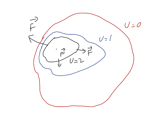
One more extremely useful observation: going back to the general case where \vec{\nabla} U \neq 0, we can see that if we take d\vec{r} in the direction perpendicular to \vec{\nabla} U, then dU = 0. If we keep traveling in the direction perpendicular to \vec{\nabla} U, we will trace out a line along which U is constant. This line is known as an equipotential. In fact, for a given \vec{\nabla} U there is a whole plane of perpendicular vectors we can choose, which means that in three dimensions we actually have a two-dimensional equipotential surface along which U doesn’t change.
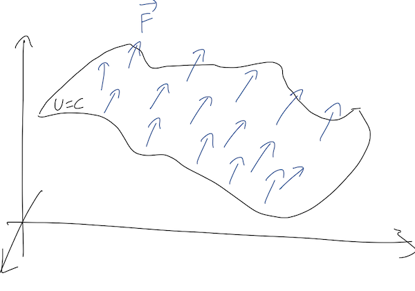
This gives us a useful way to visualize forces in two dimensions (the concept is still the same in three dimensions, but it’s very hard to draw!) Consider a point particle moving in the (x,y) plane, subject to some unknown force. In two dimensions, equipotential surfaces will just be lines, so we can make a contour plot showing the lines of constant U:
If you’ve ever read a topographic map, which shows lines of constant elevation in a top-down view, then you’re used to reading equipotential plots:
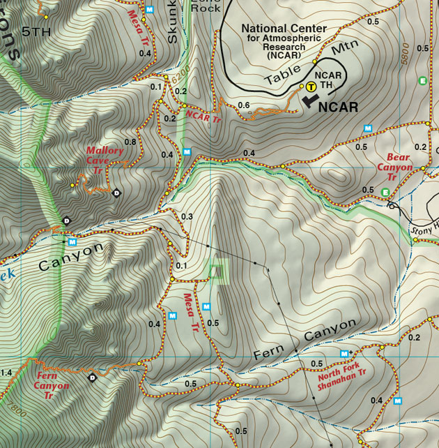
(source: https://www.latitude40maps.com/boulder-county-trails/)
Here the contours are equal height z, but since the gravitational potential U(z) \propto z, this is also a gravitational equipotential plot! This can give a useful metaphor for interpreting equipotential plots for other forces. In particular, it can help us remember the following facts:
- Equipotential lines never cross. This is basically true by definition: two different lines correspond to two different constant potential energies U_1 and U_2. Crossing would mean the potential can have two different values at the same point; our definition of a conservative force guarantees that can’t be true. For the topographic map, this is obvious - one point can’t have two heights!
- Force points “downhill”. In general, this means that since \vec{F} = - \vec{\nabla} U, the force is in the direction perpendicular to the equipotential lines and points towards smaller U. (In the topographic plot, this is literally downhill.)
- Spacing of lines tells us the magnitude of |\vec{\nabla} U|. Densely-spaced lines indicate that the potential is changing rapidly vs. position, indicating a large force. Again, this is intuitive for the topographic plot: lots of dense lines in a certain spot means a very steep slope.
Let’s gain some intuition by thinking about the details of equipotentials like this.
Here, you should complete Tutorial 4C on “Conservative Forces and Equipotential Diagrams”. (Tutorials are not included with these lecture notes; if you’re in the class, you will find them on Canvas.)
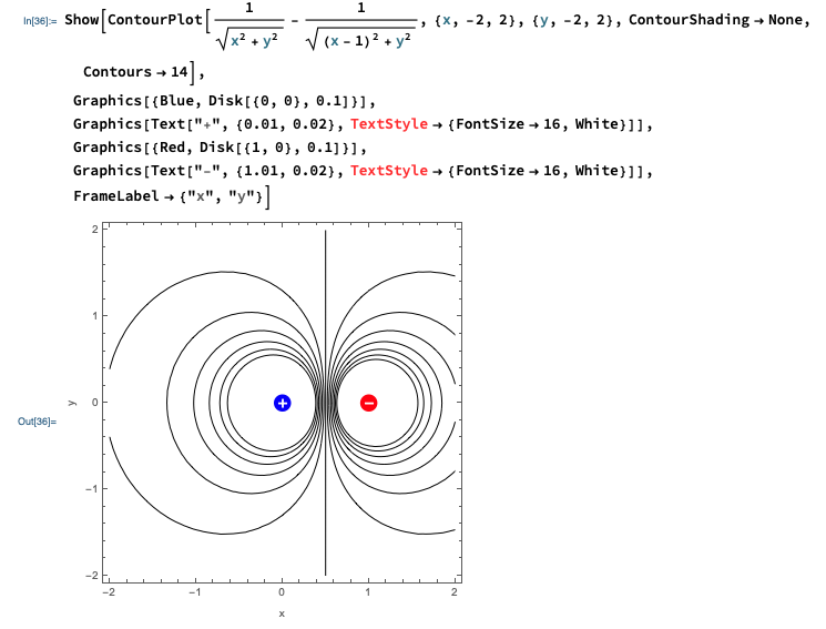
You won’t be surprised to learn that Mathematica has a function to make these plots for us, called ContourPlot[]. I won’t dwell on the details, but here’s a quick example showing how to make our own equipotential plot for a pair of electric charges.
Suppose a particle has a potential energy function of the form U(x,y,z) = 3x \cos(y/L) - 2z^2 (ignoring units for now, this is a math exercise.) What is the force?
Answer:
To find the force, we take the gradient: \vec{F} = -\vec{\nabla} U. For the gradient, we need to know the partial derivatives of U with respect to all three coordinates. We haven’t done any partial derivatives yet this semester, so let’s go through them: \frac{\partial U}{\partial x} = 3 \cos (y/L) \\ \frac{\partial U}{\partial y} = -\frac{3x}{L} \sin (y/L) \\ \frac{\partial U}{\partial z} = -4z (finding partial derivatives is easy: we just ignore everything that we’re not taking a derivative of.) Thus, the force is \vec{F} = -\vec{\nabla} U \\ = -\frac{\partial U}{\partial x} \hat{x} - \frac{\partial U}{\partial y} \hat{y} - \frac{\partial U}{\partial z} \hat{z} \\ = -3 \cos (y/L) \hat{x} + \frac{3x}{L} \sin (y/L) \hat{y} + 4z \hat{z}.
4.2.2 Cross product review
Before we move on to curl, let’s do a quick review of the cross product. Unlike the dot product, the cross product \vec{a} \times \vec{b} gives us another vector instead of a number, and in particular \vec{a} \times \vec{b} by definition is perpendicular to both \vec{a} and \vec{b}. The magnitude of the cross product is |\vec{a} \times \vec{b}| = ab \sin \theta behaving in the opposite way to the dot product; in particular, notice that |\vec{a} \times \vec{a}| is always zero. The order of the factors matters: flipping them gives back a minus sign, \vec{a} \times \vec{b} = -\vec{b} \times \vec{a}.
Now, given two different vectors \vec{a} and \vec{b}, there is a unique plane containing both of them; the direction of the cross product \vec{a} \times \vec{b} is then perpendicular to that plane. However, this isn’t quite enough information, because -\vec{a} \times \vec{b} is also perpendicular to the plane!
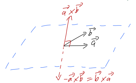
Deciding which of these two vectors to call the positive cross product is a choice of convention - which means it’s an arbitrary choice that we can make once, but then we have to keep that choice consistent. We will follow the standard physics convention, which is the right-hand rule: if you hold out your right hand with the thumb pointing in the direction of \vec{A} and your fingers in the direction of \vec{B}, then your palm points in the direction of \vec{A} \times \vec{B}. Try it with my diagram above!
The right-hand rule also fixes an ambiguity in our rectangular coordinates, which is that we could have picked either of these sets of axes:
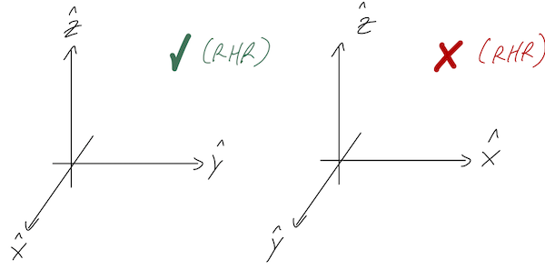
We always define our rectangular coordinates so that positive \hat{z} is a right-hand rule cross product of \hat{x} with \hat{y}. In other words, the directions of our rectangular unit vectors always satisfy: \hat{x} \times \hat{y} = \hat{z} \\ \hat{y} \times \hat{z} = \hat{x} \\ \hat{z} \times \hat{x} = \hat{y}. This is only one choice of convention, and not three; the first equation actually forces the other two to be true. An easy way to remember all three of these at once is to notice that they are all cyclic permutations: if you shift every vector to the left one spot, wrapping back around to the right at the left end, then you get the next formula.
There is a general, mechanical formula for the cross product in rectangular components, using a three-by-three matrix determinant: \vec{a} \times \vec{b} = \left|\begin{array}{ccc} \hat{x}&\hat{y}&\hat{z}\\ a_x&a_y&a_z\\ b_x&b_y&b_z\end{array}\right| \\ = (a_y b_z - a_z b_y) \hat{x} - (a_x b_z - a_z b_x) \hat{y} + (a_x b_y - a_y b_x) \hat{z}.
A couple of further identities will be especially useful in classical mechanics 2. First, the scalar triple product satisfies \vec{a} \cdot (\vec{b} \times \vec{c}) = \vec{b} \cdot (\vec{c} \times \vec{a}) = \vec{c} \cdot (\vec{a} \times \vec{b}) (cyclic permutation again!). Geometrically, this is the volume of the parallelepiped defined by the three vectors; the three forms above just correspond to picking different sides as the “base”, so they must agree.
Next, the vector triple product lets us simplify combinations of cross products: \vec{a} \times (\vec{b} \times \vec{c}) = \vec{b} (\vec{a} \cdot \vec{c}) - \vec{c} (\vec{a} \cdot \vec{b}). Taylor calls this the “BAC-CAB rule”. Think of it as a distributive rule for cross products, where each cross product becomes a dot product with one of the vectors in the parentheses, times the other vector (with an important minus sign).
Finally, taking the modulus of a cross product gives a result in terms of dot products: |\vec{a} \times \vec{b}|^2 = |\vec{a}|^2 |\vec{b}|^2 - (\vec{a} \cdot \vec{b})^2. This is sometimes called Lagrange’s identity - as if he didn’t have enough things named after him already!
4.2.3 Curl and Stokes’ theorem
The operator \vec{\nabla} can be used to define other useful quantities, in addition to the gradient. One of these useful quantities is called the curl, where the curl of \vec{v} is denoted by \vec{\nabla} \times \vec{v}.
The cross product here is taken literally: the definition of curl is that we take the cross product of the gradient vector with the second vector. Using the determinant form of the cross product, the curl is (in Cartesian coordinates only!) \nabla \times \vec{v} = \left|\begin{array}{ccc} \hat{x}&\hat{y}&\hat{z}\\ \frac{\partial}{\partial x}&\frac{\partial}{\partial y}&\frac{\partial}{\partial z}\\ v_x&v_y&v_z\end{array}\right| \\ = \left( \frac{\partial v_z}{\partial y} - \frac{\partial v_y}{\partial z} \right) \hat{x} + \left( \frac{\partial v_x}{\partial z} - \frac{\partial v_z}{\partial x} \right) \hat{y} + \left( \frac{\partial v_y}{\partial x} - \frac{\partial v_x}{\partial y} \right) \hat{z}.
Now suppose we have a force \vec{F} which is conservative. By definition, that means we can find a potential function U so that \vec{F} = -\vec{\nabla} U. But now notice what happens when we try to take the curl of \vec{F} and write it in terms of U: (\vec{\nabla} \times \vec{F})_x = \frac{\partial F_z}{\partial y} - \frac{\partial F_y}{\partial z} \\ = \frac{\partial}{\partial y} \left( -\frac{\partial U}{\partial z} \right) - \frac{\partial}{\partial z} \left( -\frac{\partial U}{\partial y} \right). But the order of partial derivatives doesn’t matter: there’s only one \partial^2 U / \partial y \partial z, so both terms are the same. Therefore, (\vec{\nabla} \times \vec{F})_x = 0. Of course, we didn’t assume anything special about the x-direction, so it won’t surprise you to know that the whole curl is in fact zero! We’ve just proved the vector identity \vec{\nabla} \times \vec{\nabla} U = 0 for any function U. This means that if we have a conservative force, then its curl must be zero: \vec{\nabla} \times \vec{F} = 0.
Curl looks like kind of a weird and arbitrary quantity, so you might wonder why we care if a force has zero curl or not. The short answer is that this identity goes both ways: if we’re given a force \vec{F}, we can calculate its curl, and if it is equal to zero then the force must be conservative. So curl allows us to test for a conservative force!
This is a big deal, because you’ll remember that the second condition for a force to be conservative was that work done is independent of path, which is something you definitely can’t test directly - there are always an infinite number of paths. But we argued that the path-independence of work is equivalent to the condition that \oint \vec{F} \cdot d\vec{r} = 0, i.e. the work vanishes on any closed path (a path that goes back to the same point, i.e. a loop.) But now we come to an important vector calculus result, Stokes’ theorem, which I will state but not prove: \oint_{\partial \mathcal{S}} \vec{F} \cdot d\vec{r} = \int \hspace{-4mm} \int_{\mathcal{S}} (\vec{\nabla} \times \vec{F}) \cdot d\vec{A}
Those are some pretty dense symbols, so in words: “Consider a finite surface \mathcal{S}, with boundary curve \partial S. The surface integral of the curl of any vector over \mathcal{S} is equal to the line integral of the same vector around the boundary \partial S.”
We don’t need to go too deep into surface integrals for our current purposes; as the name implies, they are the two-dimensional equivalent of a line integral. The important point right now is that if we have a force for which the curl \vec{\nabla} \times \vec{F} vanishes, then its line integral around any closed loop anywhere is automatically zero by Stokes’ theorem.
We can get a little bit of intuition about this visually. We can consider taking our path over a given boundary curve \partial S, and drawing a bunch of small circular paths inside of S:

Around the perimeter, we can trace out a path along the edge of the circles which is close to the black path \partial S. In the interior of this region, the paths wherever two circles meet are running in the opposite direction. This means that if we add up the line integrals over all of the circles, we get (roughly) the line integral over the outer path \partial S!
Stokes’ theorem is precisely just the infinitesmal limit of this statement. If we fill the region with an infinite number of tiny circles, then the total path over all of them combined is exactly \partial S. What is the line integral over an infinitesmal circle? Well, if it’s really tiny, a square path will be about the same:

The two vertical paths give F_y(x,y) dy + F_y(x+dx,y) (-dy) = - \frac{\partial F_y}{\partial x} dx dy while for the two horizontal paths, we get similarly F_x(x,y) (-dx) + F_x(x,y+dy) (dx) = +\frac{\partial F_x}{\partial y} dx dy. Comparing back to our formula for the curl, this is exactly -(\nabla \times \vec{F}) \cdot (\hat{z} dx dy) = -(\nabla \times \vec{F}) \cdot d\vec{A} and integrating over the whole surface S to “add up” all of the infinitesmal circles gives us the right-hand side of Stokes’ theorem.
One more detail to deal with, that you might have already noticed: I have an extra minus sign on the curl of \vec{F} here, compared to how we wrote Stokes’ theorem above. Where did the sign come from? Did I make a mistake? In fact, I chose this path intentionally. Notice that if we reversed the path \partial S, we would get an extra minus sign. But there is a notational ambiguity in our original equation: when I write \oint_{\partial \mathcal{S}} \vec{F} \cdot d\vec{r}, does \partial \mathcal{S} mean the closed path the way I drew it (running clockwise), or the reversed path (counter-clockwise)? The answer should now be clear: when we write Stokes’ theorem without an extra minus sign, we mean the counter-clockwise path. This actually follows from the right-hand rule we saw above; if we adopted a left-hand rule for cross products, then the clockwise path would be positive \partial S instead.
In summary, there are several equivalent ways to state that a force \vec{F} is conservative:
- If the work done is path-independent;
- If \vec{F} = -\vec{\nabla} U for some function U;
- If \vec{\nabla} \times \vec{F} = 0 everywhere.
Curl is much more important in electrodynamics; in mechanics, it’s mostly important as a test for conservative forces. We’ll have more use for the divergence \vec{\nabla} \cdot \vec{F} later on, but for now let’s simply move on to our next topic.
4.3 Energy and one-dimensional systems
Although we’ve been working a lot in three dimensions with our vector calculus proofs, it turns out that some of the most powerful features of energy conservation arise in one-dimensional systems. It should be noted that “one-dimensional” here doesn’t mean “only moving along a line”; it refers to any physical system in which we only need a single coordinate to tell us the full state of the system.
A basketball in freefall with no horizontal motion is a one-dimensional system (we just need the height y), but so is a pendulum (just need the angle \theta), or even a roller coaster (it’s stuck on a track, so we can describe it in terms of s, the distance along the track.) For simplicity, we’ll call our single coordinate x in the following.
What about conservative forces? Taylor shows that because one-dimensional “paths” are very simple, any force which only depends on position is automatically conservative in one dimension. So as long as there’s no dependence on other parameters like speed or time, any force in one dimension has a corresponding potential energy U(x), and F(x) = -\frac{dU}{dx}.
In one dimension, equipotential surfaces aren’t useful anymore - they would consist of some scattered points. Instead, we can visualize a problem by just plotting U(x) vs. x. For example, here is the potential U(x) = \frac{1}{2} kx^2 corresponding to a mass on a spring, which is unstretched at x=0:
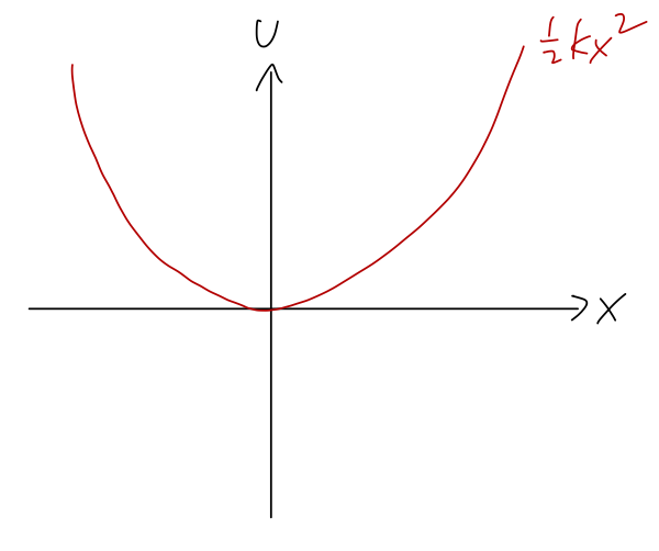
Again, the direction of the force is always “downhill”, opposite the direction of increasing U. We can also clearly see that there is an equilibrium point at x=0, where the potential is flat (dU/dx=0) and therefore the force vanishes. (Equilibrium just means that the system will stay there if we start it there at rest.)
The potential carries a lot of useful information about a physical system, even in cases where we can’t solve it completely! Once again, gravity will be a useful example and metaphor for understanding potentials in general. Imagine a roller coaster on a track. As a function of the distance x along the track, the height of the track y(x) will vary, usually in some complicated and interesting way. Since the gravitational potential is U(y) = +mgy, that means that drawing the track is the same thing as drawing the potential energy!
Suppose we have a segment of roller coaster track that looks like this:
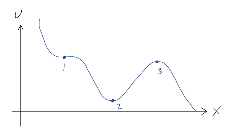
We can immediately see the points of equilibrium, marked 1, 2, and 3, where the force will vanish, and thus where the roller coaster cart would remain if it started at rest. We also get an immediate sense for the stability of these equilibria. A stable equilibrium point is one for which the system will remain near the equilibrium point if pushed slightly away; we can see that this is true at point 2, since if we give the cart a small push from this point, the force will always be directed back towards the lowest point.
An unstable equilibrium point is the opposite, a point where a small push will result in a large change in the system’s position. This is clearly the case at point 3; for a small push away from point 3, the force points away from point 3, and the coaster will accelerate away - back towards point 2, or off to the right, depending on which way we push it.
We can be more rigorous about these statements by considering a Taylor series expansion around each of these points. Let’s start with point 2, and I’ll use the shorthand notation U'(x) = dU/dx here. Since we already know that U'(x_2) = 0, the series expansion looks like U(x) \approx U(x_2) + \frac{1}{2} U''(x_2) (x-x_2)^2 + ... Now, we can’t actually compute the second derivative, but we do know from the plot that it must be positive. (Our series expansion is telling us that U(x) looks like a parabola if we get close enough to x_2, and from the plot the parabola has to be opening upwards.) So if we define U''(x_2) = +k with k>0, then U(x) \approx U(x_2) + \frac{1}{2} k(x-x_2)^2 + ... near point 2. Taking the derivative of this series gives us the force, F(x) = -\frac{dU}{dx} = -k(x-x_2). This looks exactly like a spring force; it points towards x_2, no matter what value of x we use. We can go a step further and solve for the motion. Let’s change coordinates so that u = x-x_2 is the distance to point 2. Then F(u) = -ku, and the equation of motion is m\ddot{u} = -ku. We haven’t considered general second-order ODEs yet, but we do know that this is a linear ODE, so it has a general solution containing 2 unknown constants, and we just need to find two different functions that go back to themselves with a minus sign after two derivatives. The basic trig functions both satisfy this property, so the solution is u(t) = A \cos (\sqrt{k/m} t) + B \sin (\sqrt{k/m} t). We don’t need any more detail than this: the point is that since \sin and \cos both oscillate between -1 and +1, our total solution is bounded - it will always stay within some range of point 2.
If we expand around point 3, we find an almost identical story, except that now we find U''(x_3) = -\kappa with \kappa > 0, which gives us the equation of motion m\ddot{u} = +\kappa u now with u = x-x_3. Without the minus sign, the solutions we find are exponentials instead of trig functions: u(t) = Ae^{-\sqrt{\kappa/m} t} + Be^{+\sqrt{\kappa/m} t}. The second exponential term gets arbitrarily large as t gets bigger, so our solution is indeed unstable - it will run away from point x_3. Of course, the motion isn’t exponential forever; we’re doing a series expansion around x_3, so as soon as we get far enough away that the terms we dropped from the series become important, we can’t use this simple solution for x(t) anymore.
Finally we come to point 1, which is sort of a tricky case; it is a saddle point of U(x), which means that the direction of the force depends on which way we push the cart. In physical terms, this is also an unstable equilibrium point. To see why, let’s Taylor expand one more time. We still know that U'(x_1) = 0, but we must also have U''(x_1) = 0. (You may remember from calculus that this is the condition for a saddle point. More physically, if U''(x_1) wasn’t zero, then close enough to x_1 our function would have to look parabolic, but that would mean it has to look like point 2 or point 3.) Thus, the series expansion here is U(x) \approx U(x_3) + \frac{1}{3!} U'''(x_3) (x-x_3)^3 + ... If we let U'''(x_3) = -q with q > 0 (convince yourself from the graph!), then the equation of motion is m\ddot{u} = \frac{1}{2} qu^2. We can’t solve this analytically - there is no solution using elementary functions. But we don’t need to, because it tells us what we need to know: the acceleration \ddot{u} is always positive, no matter the sign of u itself. So if we displace the cart from point 1 in either direction, it will be accelerated to the right - and since the acceleration increases as u increases, this solution is unstable and the cart moves away from point 1.
4.3.1 Total energy and turning points
Equilibrium points are local statements about a physical system, but we can also say interesting and useful things about the global behavior using the one-dimensional potential.
Let’s recap: since total energy E = T + U is conserved, if we know U(x) and the total energy, then we also know T(x). Instead of making a new plot, it’s often useful to just draw the value of E as a dotted line on the plot for U(x).
For example, let’s go back to our roller coaster and suppose the system begins at rest halfway between points 1 and 2. Then E = U(x_0), since at rest T=0. Let’s draw it on the graph:
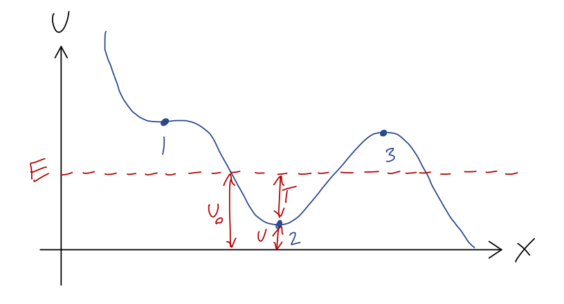
Since E = T + U and E is always the same, the difference between our dashed E line and the U(x) curve at any point is exactly the kinetic energy T! Now, since T = mv^2/2, it has the very important property that it can never be negative (note that U can be negative, and so can E, because the value U=0 is arbitrary.) But that means that we can never have U > E. So for the value of E shown, the cart can never reach point 1, point 3, or any part of the track above E!
This is a very simple but powerful observation: without knowing any of the details about how the cart moves with time, we know that its motion will never take it beyond the values of x where E = U(x) (the turning points.) The regions of the track where U > E are known as forbidden regions; we know the cart can never be found there. If all we know is E, then the cart could be anywhere else; in this example, it could be in the potential well near point 2, or it could be on the downward-sloping track to the right of point 3. If we also know where the cart starts, then we can identify it as being stuck in one of these two regions, and it can never get to the other one. (Of course, as you know from modern physics, this is only true classically; a quantum roller coaster would be able to tunnel from one region to the other.)
Here, you should complete Tutorial 4D on “One-dimensional potentials”. (Tutorials are not included with these lecture notes; if you’re in the class, you will find them on Canvas.)
We’ve previously talked about the motion of a simple pendulum, and found the equation of motion awhile ago to be \ddot{\phi} = -\frac{g}{L} \sin \phi
This is a non-linear differential equation, and there is no simple analytic solution to it at all. The usual procedure is to use the small-angle approximation, or numerical solution. But since this is a one-dimensional problem, we can instead write down the potential energy to make some useful observations!
Once again, here’s a sketch of the pendulum setup:
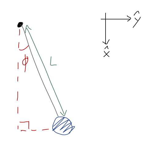
The only force acting is gravity, in the \hat{x} direction as the coordinates are drawn. Let’s set the gravitational potential to be zero at the lowest point of the pendulum, when \phi = 0. With the origin at the pendulum support, we thus have U(x,y) = mg(L-x) = mgL(1 - \cos \phi) using x = L \cos \phi. It’s always a good idea to check that the sign makes sense here, so let’s think about it: at \phi = 0, we have U = 0 as desired. At \phi = \pi/2, we have U = mgL; the gravitational potential should be larger when the bob is higher, so this also checks out.
Let’s sketch the potential as \phi changes from 0 to 2\pi:
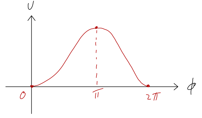
So we see two equilibrium points: in addition to the expected \phi = 0, there is also an unstable equilibrium at \phi = \pi. This might seem a little weird, but if you think about it for a moment it makes intuitive sense: at exactly \phi = \pi the pendulum is perfectly balanced straight above the support.
Although it’s easy to see graphically, let’s exercise our Taylor series abilities to check the stability or instability of the two equilibrium points. To find equilibrium points in general, we solve for where the gradient of U vanishes, or: \frac{dU}{d\phi} = 0 = mgL \sin \phi which has solutions at \phi = 0, \pi, 2\pi, ..., matching the points I already marked on the graph. Next, if we series expand the potential first at \phi = 0, we have U(\phi) \approx U(0) + \frac{1}{2} U''(0) \phi^2 + ... \\ = mgL(1 - \cos 0) + \frac{1}{2} (mgL \cos 0) \phi^2 + ... \\ = \frac{1}{2} mgL \phi^2 + ... which is indeed a stable equilibrium, since the coefficient of \phi^2 is positive. Note that I skipped the U' term in the expansion, since I already know it’s zero at this point. Let’s repeat the exercise at \phi = \pi, U(\phi) \approx U(\pi) + \frac{1}{2} U''(\pi) (\phi-\pi)^2 + ... \\ = mgL(1 - \cos \pi) + \frac{1}{2} (mgL \cos \pi) (\phi-\pi)^2 + ... \\ = 2mgL - \frac{1}{2} mgL (\phi-\pi)^2 + ... which is indeed unstable: the potential looks like a downwards parabola near the point, and if we compute the force F(\phi) = -\frac{dU}{d\phi} = mgL(\phi - \pi) it will always point in the same direction as \phi if we move slightly away from the equilibrium, and we will be pushed away.
Moving beyond equilibrium, we can also use conservation of energy and turning points to say useful things about the motion, without having to assume a small angle. Suppose the pendulum starts at \phi = 0, and we give it a push so that it starts moving with initial speed v_0. What does its motion look like? The total energy is just T at \phi = 0, so we have E = T + U \\ \frac{1}{2} mv_0^2 = T + mgL(1 - \cos \phi) The turning points \phi_T occur where T = 0, or \frac{1}{2} mv_0^2 = mgL (1 - \cos \phi_T) \\ 1 - \cos \phi_T = \frac{v_0^2}{2gL} \\ \Rightarrow \cos \phi_T = \left( 1 - \frac{v_0^2}{2gL} \right). So although we don’t know the detailed motion as a function of time, it’s easy to find the maximum possible angle the pendulum will reach based on the initial speed. Notice that this works for any angle, but only for v_0^2 < 4gL, at which point \phi_T = \pi. For even larger initial speeds, there is no solution: we just have E > U everywhere, and the pendulum will just spin in a circle forever, in the absence of other forces.
If we really want to know about the motion as a function of time, there’s one more nice trick we can do in one dimension. For any potential at all, the relation E = T + U in one dimension can be rewritten as: \frac{1}{2} m \dot{x}^2 = E - U(x). which we can solve for \dot{x}: \dot{x} = \pm \sqrt{\frac{2}{m}} \sqrt{E - U(x)} (we would need extra information to figure out the sign, since T is the same for +\dot{x} and -\dot{x}.) This is a first order and separable ODE - no matter how complicated U(x) is! So we can use it to write down a completely general solution: if x(0) = x_0, then t(x) = \pm \sqrt{\frac{m}{2}} \int_{x_0}^x \frac{dx'}{\sqrt{E-U(x')}} which we then have to invert to get x(t).
For the pendulum, this becomes t(\phi) = \pm \sqrt{\frac{m}{2}} \int_{\phi_0}^\phi \frac{d\phi'}{\sqrt{E - mgL(1 - \cos \phi')}} This is, unfortunately, one of those integrals that you can’t actually do: it is used to define a special function called an elliptic function, which is the solution to the pendulum at all angles. So we didn’t get something for nothing in this case. On the other hand, this can be a convenient way to do a numerical solution, since you don’t need an ODE solver like Mathematica - you just need to do an integral.
Here, you should complete Tutorial 4E on “One-dimensional potentials (part 2): Morse potential”. (Tutorials are not included with these lecture notes; if you’re in the class, you will find them on Canvas.)
Taylor explores a few other special topics in energy conservation, including the use of time-dependent potential energies (Taylor 4.5) and some more explorations of equilibrium and one-dimensional systems (4.7); I encourage you to read about these for your interest, but we won’t go into them in any detail. Instead, we’ll continue with his discussion of central forces, which will lead us into a detailed case study of the most important fundamental force in mechanics: gravity.