5 Central forces and gravity
The most important forces in physics, gravity and electric force, have some important features in common. They are both generated at a distance from a source (mass for gravity, electric charge for electric force), and the resulting force is always directly towards the source. This makes them both examples of “central forces”, a structure which leads to important and powerful simplifications.
5.1 Central forces
A central force is one for which in some choice of coordinates, \vec{F}(\vec{r}) = f(\vec{r}) \hat{r}. The key point here is that the origin (i.e. the center of our coordinate system) is the source providing our central force, and the force at any point \vec{r} always points towards or away from this center. This should remind you a bit of drag forces, which we argued were always in the direction of \hat{v} (or opposite \hat{v}, more precisely.) In both cases, we have a specific direction for the force by identifying where it comes from (motion for air resistance, and the source object for central force.)
We’ll deal with gravity in great detail soon. As touches on above, another good example that you already know of a central force is just the electric force: if I put a charge Q at the origin, then the force on a second charge q sitting at point \vec{r} is \vec{F}_e(\vec{r}) = \frac{kqQ}{r^2} \hat{r}. As Taylor observes, this (along with gravity, which has the same r dependence) is a slightly more specialized version of a central force, because f(\vec{r}) = f(r), i.e. the magnitude of the force only depends on the distance between the charges. This is an example of spherical symmetry, or rotational invariance: in spherical coordinates, we can rotate our test charge q around in \theta and \phi as much as we want, and as long as r is held fixed the force magnitude is the same (although the direction changes so it’s always pointing out from the origin.) As we’ll prove in a moment, this is related to the question of whether or not we have a conservative central force. A static electric force is definitely conservative!
5.1.1 Gradient and curl in spherical coordinates
To study central forces, it will be easiest to set things up in spherical coordinates, which means we need to see how the curl and gradient change from Cartesian. Let’s talk through the derivation for the gradient - although this is something you can always look up, it’s actually pretty easy, and the formula that you look up won’t seem so arbitrary. Remember that in our derivation of gradient, we found the following infinitesmal relationship: dU = \vec{\nabla} U \cdot d\vec{r}. To proceed, we need d\vec{r} in spherical coordinates. The derivation in full is included below, if you want to see it - it’s not that bad, but it requires a bit of algebra. The result is: d\vec{r} = dr\ \hat{r} + r d\theta\ \hat{\theta} + r \sin \theta\ d\phi\ \hat{\phi}.
We start with the observation that in spherical coordinates, \vec{r} = r\hat{r}. Taking the derivative with respect to some parameter s, \frac{d\vec{r}}{ds} = \frac{dr}{ds} \hat{r} + r \frac{d\hat{r}}{ds}. Next, we can relate the unit vector \hat{r} back to Cartesian coordinates: \hat{r} = \frac{1}{r} \left( x \hat{x} + y \hat{y} + z \hat{z} \right) \\ = \sin \theta \cos \phi \hat{x} + \sin \theta \sin \phi \hat{y} + \cos \theta \hat{z}. We can take a derivative with respect to s here, but it’s better to remember that we eventually want our answer in terms of spherical unit vectors. Remember that we define the unit vectors as pointing in the direction of change with respect to a certain coordinate, so we can find them by looking at the derivatives of \hat{r}: \frac{d\hat{r}}{d\theta} = \cos \theta \cos \phi \hat{x} + \cos \theta \sin \phi \hat{y} - \sin \theta \hat{z} \\ \frac{d\hat{r}}{d\phi} = - \sin \theta \sin \phi \hat{x} + \sin \theta \cos \phi \hat{y} and computing the lengths, \left| \frac{d\hat{r}}{d\theta} \right| = \cos^2 \theta (\cos^2 \phi + \sin^2 \phi) + \sin^2 \theta = 1 \\ \left| \frac{d\hat{r}}{d\phi} \right| = \sin^2 \theta (\sin^2 \phi + \cos^2 \phi) = \sin^2 \theta Now we use the chain rule: \frac{d\hat{r}}{ds} = \frac{d\hat{r}}{d\theta} \frac{d\theta}{ds} + \frac{d\hat{r}}{d\phi} \frac{d\phi}{ds} \\ = \left| \frac{d\hat{r}}{d\theta} \right| \hat{\theta} \frac{d\theta}{ds} + \left| \frac{d\hat{r}}{d\phi} \right| \hat{\phi} \frac{d\phi}{ds} on the last line using the definition of the unit vectors, \hat{\theta} = \frac{d\vec{r}/d\theta}{|d\vec{r}/d\theta|} = \frac{d\hat{r}/d\theta}{|d\hat{r}/d\theta|} where the second equality comes from the fact that the difference between \vec{r} and \hat{r} is a factor of the radius r, which doesn’t depend on the angle and so just cancels out. Combining our results above, we have \frac{d\hat{r}}{ds} = \frac{d\theta}{ds} \hat{\theta} + \sin \theta \frac{d\phi}{ds} \hat{\phi} or going all the way back to the start and cancelling out the ds infinitesmals, d\vec{r} = dr \hat{r} + r d\theta \hat{\theta} + r \sin \theta d\phi \hat{\phi}. This was a little bit of an algebra grind, but it’s been a little while since we’ve done these sorts of coordinate manipulations so I thought the practice would be good!
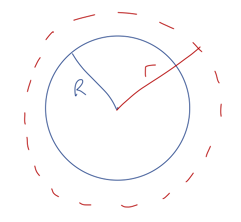
If you prefer a geometric derivation, Taylor does it that way without the algebra. In fact, it’s pretty easy to see that this form makes sense from a little sketch:
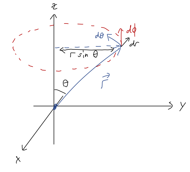
At fixed r, in the \theta direction, we’re always moving around a big circle of radius r, so the infinitesmal arc length that we travel is ds = r d\theta. In the \phi direction we’re also tracing out a circle, but the size of that circle depends on \theta, so ds = \rho d\phi = r \sin \theta d\phi.
Next, to work out how the function U changes with respect to coordinates, we just apply the chain rule to find dU = \frac{\partial U}{\partial r} dr + \frac{\partial U}{\partial \theta} d\theta + \frac{\partial U}{\partial \phi} d\phi. Notice there are no extra factors or coordinate changes to worry about - since U is just a scalar function, the chain rule applies in this same simple way no matter what! Now we rewrite the original equation: dU = \vec{\nabla} U \cdot d\vec{r} \\ \frac{\partial U}{\partial r} dr + \frac{\partial U}{\partial \theta} d\theta + \frac{\partial U}{\partial \phi} d\phi = (\vec {\nabla} U) \cdot \left( dr \hat{r} + r d\theta \hat{\theta} +r \sin \theta d\phi \hat{\phi} \right) and just matching the dr, d\theta, d\phi terms on both sides, we find \vec{\nabla} U = \frac{\partial U}{\partial r} \hat{r} + \frac{1}{r} \frac{\partial U}{\partial \theta} \hat{\theta} + \frac{1}{r \sin \theta} \frac{\partial U}{\partial \phi} \hat{\phi}.
Not bad at all! The bad news is that we can’t simply derive the curl or divergence from the gradient in spherical or cylindrical coordinates. This is basically for the same reason that Newton’s laws become more complicated in these coordinate systems: the unit vectors themselves become coordinate-dependent, so extra terms start to pop up related to derivatives acting on unit vectors.
The correct way to derive the curl in spherical coordinates would be to start with the Cartesian version and carefully substitute in our coordinate changes for the unit vectors and for (x,y,z) \rightarrow (r,\theta,\phi). This is straightforward but tedious, so I’ll skip to the result: the curl in spherical coordinates takes the form, in determinant notation, \vec{\nabla} \times \vec{A} = \frac{1}{r^2 \sin \theta} \left| \begin{array}{ccc} \hat{r} & r \hat{\theta} & r \sin \theta \hat{\phi} \\ \frac{\partial}{\partial r} & \frac{\partial}{\partial \theta} & \frac{\partial}{\partial \phi} \\ A_r & r A_\theta & r \sin \theta A_\phi \end{array} \right|
Let’s use this to compute the curl of central force vector \vec{F}(\vec{r}) = f(\vec{r}) \hat{r} in spherical coordinates: \vec{\nabla} \times \vec{F}(\vec{r}) = \frac{1}{r^2 \sin \theta} \left| \begin{array}{ccc} \hat{r} & r\hat{\theta} & r\sin \theta \hat{\phi} \\ \frac{\partial}{\partial r} & \frac{\partial}{\partial \theta} &\frac{\partial}{\partial \phi} \\ f(\vec{r}) & 0 & 0 \end{array} \right| \\ = \frac{1}{r \sin \theta} \frac{\partial f}{\partial \phi} \hat{\theta} - \frac{1}{r} \frac{\partial f}{\partial \theta} \hat{\phi}. So we can see right away that the condition for the curl to vanish - and therefore for \vec{F}(\vec{r}) to be conservative - is that both \partial f/\partial \phi and \partial f/\partial \theta should be zero, or in other words the magnitude should only depend on the radius, f(\vec{r}) = f(r). You can also prove this by using the gradient and matching on to the fact that \vec{F} has to point in the \hat{r} direction; convince yourself from the formula for \vec{\nabla} U we found, or read the argument in Taylor.
A central force \vec{F}(\vec{r}) = f(\vec{r}) \hat{r} is conservative if (and only if) it depends only on distance to the source: f(\vec{r}) = f(r).
5.1.2 Two-particle central forces
Conservative central forces are common in physics, particularly for fundamental forces: both electric force and gravitational force are central and conservative. One of the really nice features of such a force is that since the magnitude only depends on r, the distance to the source, many aspects of their physics can be treated as one-dimensional; we’ve already seen how that can be a really powerful simplification.
However, this setup so far forces a coordinate choice on us: we have to put our source at the origin. But what if we have two particles that are both sources, and are both moving - how can we describe their effects on each other through a central force? More generally, what if we have an extended source which is larger than a point - where do we put the origin?
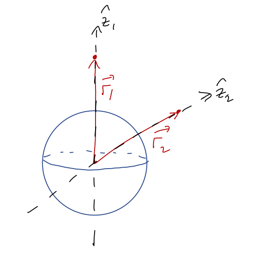
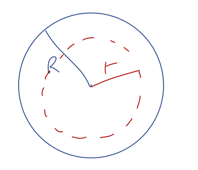
We’ll start by generalizing to the two-particle case, which will be the hard part; taking the next step to extended sources will be easy. We start with two particles labelled 1 and 2, at positions \vec{r}_1 and \vec{r}_2 like this:
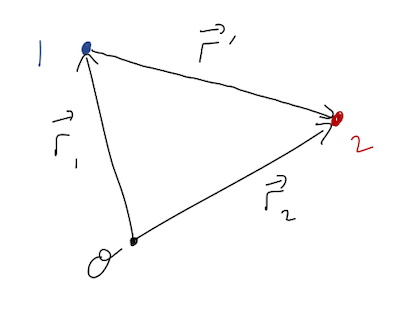
No external forces are present, but as shown, we assume that the particles are exerting a central force on one another. Defining the \hat{r}' vector pointing from 1 to 2 as shown, we have from the definition of a central force \vec{F}_{12} = f(\vec{r}') \hat{r}' \\ \vec{F}_{21} = -f(\vec{r}') \hat{r}' where we notice that Newton’s third law requires the magnitude to be the same function, so that these are equal and opposite. Now, \vec{r}' isn’t some unknown, it’s related to the positions of our two objects: \vec{r}' = \vec{r}_1 - \vec{r}_2 (easier to see in the form \vec{r}_1 + \vec{r}' = \vec{r}_2), and for the corresponding unit vector \hat{r}' = \frac{\vec{r}'}{|\vec{r}'|} = \frac{\vec{r}_1 - \vec{r}_2}{|\vec{r}_1 - \vec{r}_2|}. Since the central force only acts in the \vec{r}' direction, the point is that we can just solve for the relative motion of our two objects, and we’re back to having just one vector to worry about instead of two. So we don’t have to push one object to the origin for a central force to be a useful description of two objects - we just focus on their relative position.
You might object that just knowing the relative position isn’t enough information! We have two particles, which means we need 6 numbers to describe where they both are at any given moment, but \vec{r}' only has three components. In fact, we can get the other three components using the center of mass: because we’ve specified no external forces, we have for the CM position M \ddot{\vec{R}} = \vec{F}_{\textrm{ext}} = 0 which gives us the other three equations we need to fully keep track of everything.
What if we have not just a central force, but a conservative force? We know that f(\vec{r}') becomes just f(r') - that is, the force will only depend on the distance between our two particles and nothing else. As a result, we can write a single potential energy function U(r') that will describe the force f(\vec{r}')!
To get the individual forces from the potential, we take gradients with respect to each coordinate: \vec{F}_{12} = -\vec{\nabla}_1 U(r') \\ \vec{F}_{21} = -\vec{\nabla}_2 U(r') where the subscript gradient means “take derivatives with respect to the given coordinate”, for example in Cartesian coordinates \vec{\nabla}_1 = \frac{\partial}{\partial x_1} \hat{x}_1 + \frac{\partial}{\partial y_1} \hat{y}_1 + \frac{\partial}{\partial z_1} \hat{z}_1 ignoring the coordinates of \vec{r}_2. It’s easy to show from the definition of \vec{r}' that this definition gives us equal and opposite forces as required by the third law (try it yourself!)
Taylor has a very thorough discussion of how all of this generalizes beyond two particles, to the general N-particle case: the punchline is that we can always define a combined potential energy U for all our particles, and the force on any given particle is \vec{F}_\alpha = -\vec{\nabla}_\alpha U(\vec{r}_1, \vec{r}_2, ..., \vec{r}_N) and the total energy E = T_1 + T_2 + ... + T_N + U is always conserved (if the forces involved are conservative - which we’ve sort of assumed by writing a U in the first place, but there are some edge cases like time-dependent potential energies that Taylor talks about.)
I will just let you read the Taylor derivation and not go over it here; it’s an important fundamental result, but it doesn’t really show off any math that we haven’t seen before, and it’s not something we’ll need to work with practically. But the upshot is very important:
Given a conservative, central force, the combined force on a single point mass (at position \vec{r}) due to all other sources in the system can be described in terms of a single potential energy function U(\vec{r}).
This is a very useful observation, because it lets us deal with extended sources - realistic objects that emit a force, instead of only point sources. With this result in hand, let’s move on to consider a single conservative, central force in detail: gravity!
5.2 Gravity
Our starting point is Newton’s general law of gravitation. If we have a source mass M at the origin, and a test mass m at \vec{r}, the force of gravity acting on the test mass is \vec{F}_g = -\frac{GMm}{r^2} \hat{r}. The “gravitational charge” of an object is just its mass. Since mass is always positive, the force of gravity is always attractive - it pulls the two objects together, or in this case, pulls the mass m towards M at the origin. The constant G is known as the gravitational constant, Newton’s constant or just “big G”; its best value, according to NIST CODATA, is G = 6.67430(15) \times 10^{-11}\ {\textrm{m}}^3 / {\textrm{kg}} / {\textrm{s}}^2. The corresponding potential energy function is U(r) = -\frac{GMm}{r} We can add an arbitrary constant to it; the choice above with no constant corresponds to choosing our zero point at infinity, i.e. \lim_{r \rightarrow \infty} U(r) = 0.
Take special note that both \vec{F}_g and U(r) are negative, despite the relationship \vec{F} = -\nabla U! Mathematically, this happens because the derivative of 1/r pops out a extra minus sign, which cancels the other minus sign in the definition of force. You can also remember the sign on physical grounds: it takes work to push two massive objects apart against gravity, so U should increase as r increases, which it does with the minus sign.
The gravitational force closely resembles the electric force, and in a similar way to the electric example, we can define a gravitational field \vec{g} by dividing out the “charge” (the mass in this case), such that \vec{F}_g = m\vec{g}. From above, the gravitational field generated by a point mass M is then \vec{g} = -\frac{GM}{r^2} \hat{r}.
There isn’t a whole lot of interesting physics we can do with just two masses, as it turns out. (Well, we could derive Kepler’s laws for the motion of planets in the solar system, but that turns out to be much nicer with some extra math tools that you’ll get next semester.) So what happens if we have multiple sources? Since multiple forces acting on a simple object just add together, we can also add together the gravitational fields from multiple sources to get a single, combined field: \vec{g} = \vec{g}_1 + \vec{g}_2 + ... = -\frac{GM_1}{r_1^2} \hat{r}_1 -\frac{GM_2}{r_2^2} \hat{r}_2 + ...
This is the starting point we need to talk about extended sources, which will let us do some realistic applications of gravity, such as the Earth’s gravitational field.
5.2.1 Extended sources of gravity
To deal with realistic objects, we’d like to be able to calculate the gravitational field due to a continuous object with some density. Recalling our previous example of finding the center of mass, we can think of this as just adding up all of the contributions from infinitesmal bits of mass dm inside of an object. For the center of mass, recall we had M = \sum_\alpha m_\alpha,\ \ \vec{R} = \frac{1}{M} \sum_\alpha m_\alpha \vec{r}_\alpha which became for continuous objects M = \int dm = \int \rho(\vec{r}) dV,\\ \vec{R} = \frac{1}{M} \int \vec{r} dm = \frac{1}{M} \int \vec{r} \rho(\vec{r}) dV.
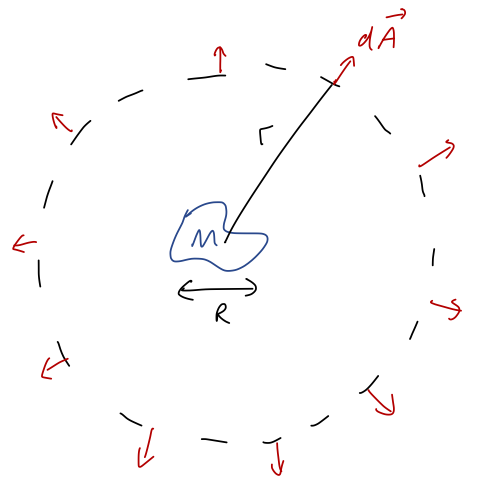
Similarly, for an extended massive source, we can add up all of the contributions to the gravitational field from individual pieces. However, this is going to be a little more complicated, so we should start with a diagram:
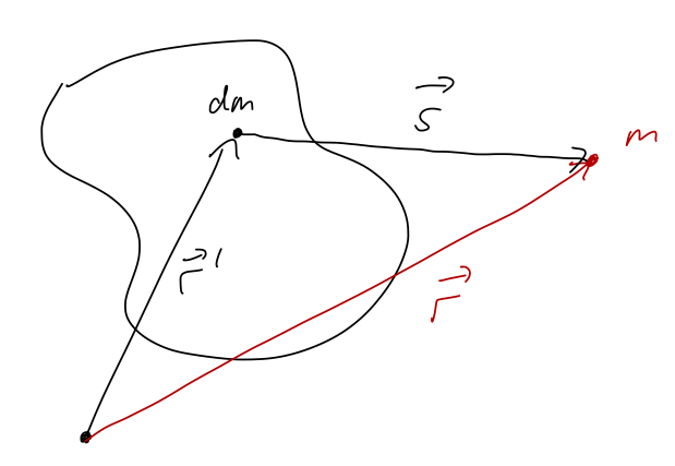
As pictured, we have to keep track of the location \vec{r}' of our source mass, but also the position \vec{r} where we want to know the field. As a sum over individual masses m_\alpha, we have
\vec{g} = \sum_\alpha -\frac{Gm_\alpha}{|\vec{s}_\alpha|^2} \hat{s}_\alpha where \vec{s} = \vec{r} - \vec{r}'_\alpha is the vector pointing from the source mass \alpha to the position \vec{r}. (Some books will refer to this using a funny-looking script r; I think this is confusing, and I also don’t know how to typeset the weird r, so I’ll use s.)
We find the continuous version by replacing m with the density \rho: \vec{g}(\vec{r}) = -G \int \frac{dm}{|\vec{s}|^2} \hat{s} \\ = -G \int \frac{dV' \rho(\vec{r}')}{|\vec{r} - \vec{r}'|^3} (\vec{r} - \vec{r}') where I’ve written out \hat{s} in terms of the other vectors, which gives us an extra factor of 1/|\vec{s}|. As the prime on dV' indicates, we’re integrating over all possible positions \vec{r'} of the source mass dm. We can do a u-substitution to think of the integral as being over the relative position vector \vec{s}, but that hides the dependence on \vec{r'} which can be confusing.
This looks pretty horrible compared to the center of mass integral! Much of the complication comes from the fact that we have a second vector \vec{r} in addition to the one that we’re trying to integrate over. We’ll do a couple of examples, but I’ll emphasize from the start that it is very important to make sketches and think carefully about these vectors when trying to calculate \vec{g}!
Symmetry will also be very useful, as with the center of mass. In particular, suppose we are at the origin and there are two equal pieces of mass at +\vec{s} and -\vec{s}, exactly on opposite sides:
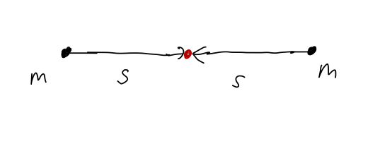
Then the total gravitational field is, taking the horizontal direction to be the x-axis, \vec{g} = -\frac{Gm}{s^2} \hat{x} - \frac{Gm}{s^2} (-\hat{x}) = 0. In other words, just as we saw for the CM position, the contributions of two equal masses at opposite positions to the \vec{g} field cancel exactly. This reflection-symmetry observation will extend to a whole object: if we have two solid hemispheres with the same mass and shape, then at the point exactly in between their centers, \vec{g} = 0 without having to calculate anything.
This can also work component by component. If we have our two equal masses at (+x',0,0) and (-x',0,0), and we’re interested in the gravitational field along the y axis:

The distance s to both sources is the same again, but now the directions are slightly different. Worrying about the \hat{s} vector (which we’ll define with respect to the left source to be consistent with signs), we have:
g_x = -\frac{GM}{s^2} (\hat{s}_x - \hat{s}_x) = 0, \\ g_y = -\frac{GM}{s^2} (\hat{s}_y + \hat{s}_y) \neq 0.
In words: the magnitude of the field is the same from both sources, but the y-components add since they both point in the same direction (downwards), so g_y is not zero.
Here, you should complete Tutorial 4F on “Gravitational fields”. (Tutorials are not included with these lecture notes; if you’re in the class, you will find them on Canvas.)
Let’s try to apply our setup to a real example of finding \vec{g} for an extended object (not just point masses.) Suppose we have a solid but very thin disk of constant area mass density \sigma and radius R.
To deal with a thin disk, our integral over dV will become just a two-dimensional area integral dA, since the z-direction is infinitesmally thin. (If you’re not happy with this hand-waving approximation, you can calculate the three-dimensional version of this for a height h, and then take the limit h \rightarrow 0. You should get the same results we’re about to find.)
Now, as with the center of mass, we can view the equation for \vec{g} as just three separate integrals to do for each of the components g_x, g_y, g_z. In general, we need to calculate all three of them, but symmetry can save us by telling us certain components are automatically zero. However, things are complicated by the fact that we have to choose the point \vec{r} to calculate the field at. For a completely arbitrary point in space, symmetry won’t help us for the disk!
But let’s say we want to calculate the field directly above the center of the disk, along the z-axis:
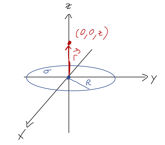
Then we have \vec{g}_x = \vec{g}_y = 0 thanks to reflection symmetry (remember, it’s the reflection of the relative \vec{s} vector that matters, which is why we had to specify \vec{r} = z\hat{z} first!) Let’s convince ourselves by actually setting up one of the integrals: g_x = -G \int \frac{dA' \sigma}{|\vec{r} - \vec{r}'|^3} (\vec{r} - \vec{r}')_x \\ = G \sigma \int \frac{dA' x'}{(x'^2 + y'^2 + z^2)^{3/2}} using \vec{r} - \vec{r}' = -x' \hat{x} - y' \hat{y} + z \hat{z}, from the diagram. Now, this is already good enough to see the cancellation: because the integrand has a single x' upstairs, for every point on the disk at (+x', +y') there will be an equal and opposite contribution from (-x',y'), so the whole thing will be zero. To see it even more explicitly, we should really change to cylindrical coordinates (\rho', \phi') inside the integral: g_x = G \sigma \int_0^{2\pi} d\phi' \int_0^R d\rho' \frac{\rho'^2 \cos \phi'}{(\rho'^2 + z^2)^{3/2}} The \phi' integral is the one that matters, and it’s easy to do: we have \int_0^{2\pi} d\phi' \cos \phi' = \left. \sin \phi'\right|_0^{2\pi} = 0.
Since the choice of x-direction vs. y-direction on a disk is totally arbitrary, clearly the same setup will give us g_y = 0 as well.
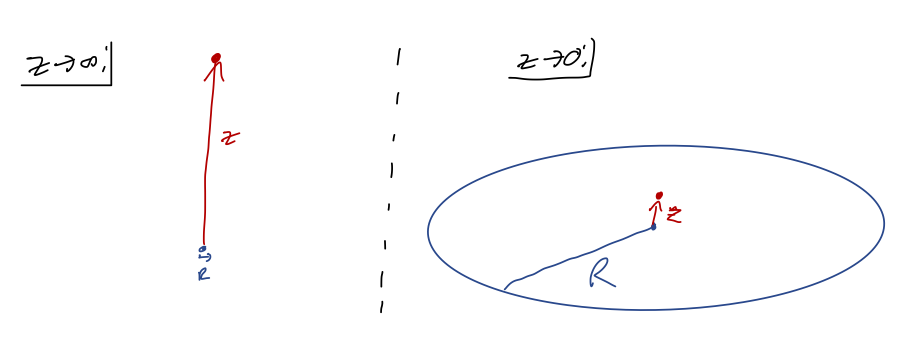
Now let’s move on to the non-zero part of the field, g_z. Since we’ve already gone through the details of the setup for x, it should be easy to see that g_z = -G \sigma \int_0^{2\pi} d\phi' \int_0^R d\rho' \frac{\rho' z}{(\rho'^2 + z^2)^{3/2}} \\ = -2\pi G \sigma z \int_0^R \frac{d\rho' \rho'}{(\rho'^2 + z^2)^{3/2}}. This is actually a very friendly integral for u-substitution! Let’s pick u = \rho'^2 + z^2, which gives du = 2\rho' d\rho'. Then g_z = -2\pi G \sigma z \int_{z^2}^{R^2 + z^2} \frac{du/2}{u^{3/2}} \\ = -\pi G \sigma z \left( \left. -\frac{2}{u^{1/2}} \right|_{z^2}^{R^2+z^2} \right) \\ = 2\pi G \sigma z \left( \frac{1}{\sqrt{R^2 + z^2}} - \frac{1}{|z|} \right). \\ We could replace the density \sigma with the total mass M; since it’s a two-dimensional density, we have M = \sigma \pi R^2. But there’s no normalizing 1/M like there is for the center of mass, so for this calculation it’s fine to just leave it in terms of \sigma in general.
The other limit to consider is z \rightarrow \infty. This means that z \gg R, which we can use to series expand the first term in the field: \frac{1}{\sqrt{R^2 + z^2}} = \frac{1}{|z|} \frac{1}{\sqrt{1 + (R/z)^2}} Let’s use the binomial formula to expand, (1+z)^n = 1 + nz + \frac{n(n-1)}{2} z^2 + ... which leads to, just keeping the first two terms, \frac{1}{\sqrt{R^2 + z^2}} \approx \frac{1}{|z|} \left(1 - \frac{R^2}{2z^2} + ... \right) The 1/|z| terms cancel off, and we’re left with g_z \rightarrow 2\pi G \sigma \frac{z}{|z|} \left( -\frac{R^2}{2z^2} + ... \right) Now it’s useful to substitute in M = \pi R^2 \sigma, which will absorb the R^2 factor and leave us with g_z \rightarrow -\frac{GM}{z^2} \frac{z}{|z|} or \vec{g} = -GM/z^2 \hat{r}, along the z-axis. So in this limit, the leading dependence on R vanishes and we just recover the single point-particle form of the gravitational field! This makes a lot of sense: if we’re really, really far away from the disk, then the fact that it’s an extended object doesn’t really matter - in fact, from far enough away we probably wouldn’t be able to tell that it has any radius, we would just see a point.
5.2.2 Gravitational potential
So far, we haven’t really used the fact that gravity is a conservative force. In fact, being able to write a potential energy function U(\vec{r}) can actually save us a lot of work when dealing with extended objects! Recall that the potential energy for a single test mass m in the gravity field of a source mass M is U(r) = -\frac{GMm}{r}. When we have multiple sources, as we discussed above for any conservative central force, we simply add up the potentials!
One more definition before we continue: like the force, the potential energy depends on the test mass m, but in a very trivial way. It’s often useful to factor out the m so we can calculate a function that only depends on the sources, which we can then apply to any test mass (or collection of test masses.) So just like we defined \vec{F}_g = m\vec{g}, we now define the gravitational potential for a point source to be \Phi(r) = -\frac{GM}{r} so that U(r) = m\Phi(r). We can immediately see that \vec{g} = -\vec{\nabla} \Phi, so this gives us another way to find the gravitational field.
Potential is an unfortunate name for the quantity \Phi; it is not a potential energy, since it has the wrong units! Taking the combination U = m\Phi gives us an actual potential energy. This is completely analogous to the electric potential V(r), which is also not a potential energy - but the combination qV is.
Now if we have an extended object, as we saw before:
then the potential at position \vec{r} due to the infinitesmal source dm is d\Phi(\vec{r}) = -\frac{G dm}{s} = -\frac{G dm}{|\vec{r} - \vec{r}'|}, and thus the total potential is \Phi(\vec{r}) = -G \int \frac{dV' \rho(\vec{r}')}{|\vec{r} - \vec{r}'|}. This is much nicer to evaluate than the integrals we had to do for \vec{g}! Now we have no vector components to worry about - just a single scalar quantity. We can then take the gradient of our result (with respect to \vec{r}) to find the gravitational field \vec{g}.
Here, you should complete Tutorial 4G on “Gravitational potential”. (Tutorials are not included with these lecture notes; if you’re in the class, you will find them on Canvas.)
Now let’s do an example to see how this approach works in more detail.
Let’s find the \vec{g} field due to a spherical shell of mass M (and constant mass density \sigma), using the gravitational potential \Phi. Once again, we’ll consider a target point on the z-axis, so \vec{r} = z\hat{z}.
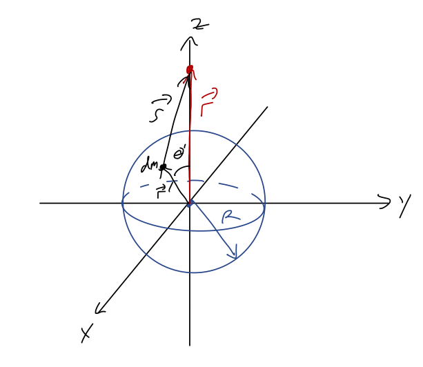
We start by setting up the integral, using the sketch as a guide: \Phi(\vec{r}) = -G \int \frac{dA' \sigma}{|\vec{r} - \vec{r}'|}. Let’s work in spherical coordinates since we have a sphere. The vector \vec{r}' has length R, but is at arbitrary spherical angles \theta, \phi. In order to proceed, we’ll need to find the length of the vector \vec{r} - \vec{r}'. The geometry is a bit tricky, although if you make a sketch and remember the law of cosines, it’s straightforward to find.
I personally can never remember the law of cosines, so I prefer to just write out the two vectors and take the difference! Using spherical coordinates but Cartesian basis vectors, we have:
\vec{r}' = R \sin \theta' \cos \phi' \hat{x} + R \sin \theta' \sin \phi' \hat{y} + R \cos \theta' \hat{z} and much more simply, \vec{r} = z \hat{z}. So, taking the difference and then the squared length: |\vec{r} - \vec{r}'|^2 = (r' \sin \theta' \cos \phi')^2 + (r' \sin \theta' \sin \phi')^2 + (z - r' \cos \theta')^2 \\ = r'^2 + z^2 - 2zr'\cos \theta'.
You might wonder, why are we mixing spherical and Cartesian coordinates here, instead of just working with spherical basis vectors as well? The reason is that spherical basis is great for any single vector, but with two vectors to deal with here it’s not so useful!
In spherical coordinates, the reference point is at \vec{r} = z \hat{\rho}, and the object point is at \vec{r}' = R \hat{\rho}'. But since these are two different vectors, they have two different spherical unit vectors! We could try to figure out how \hat{\rho} and \hat{\rho}' are related, but we need a common set of basis vectors to do it - probably just the Cartesian basis we’re using anyway for this problem.
Now we can set up our integral for \Phi(z). Since we’re working with a shell, this will be an area integral over the two spherical angles:
\Phi(z) = -G \sigma \int_0^{2\pi} d\phi' \int_0^\pi d\theta' \frac{R^2 \sin \theta'}{\sqrt{R^2 + z^2 - 2zR \cos \theta'}}.
The integral over \phi' is trivial, and just pops out a factor of 2\pi, so the only work we have left is the \theta' integral. This integral is actually a little tricky, simply because you have a good chance of getting stuck if you’re used to just plugging things in and letting Mathematica deal with them!
The good news is that there is a pretty obvious u-substitution to do. Since almost everything in the square root is constant, we can write u = R^2 + z^2 - 2zR \cos \theta' \Rightarrow du = 2zR \sin \theta' d\theta' The new limits of integration will be \theta'=0 \Rightarrow u=(z-R)^2, \\ \theta' = \pi \Rightarrow u = (z+R)^2.
With the \sin \theta' already upstairs, this simplifies really nicely: \Phi(z) = -2\pi \sigma G \int_{(z-R)^2}^{(z+R)^2} \frac{R^2 du}{2zR} \frac{1}{\sqrt{u}} \\ = -\pi \sigma G \frac{R}{z} \left(2 \left.\sqrt{u}\right|_{(z-R)^2}^{(z+R)^2}\right) \\ = -2\pi \sigma G \frac{R}{z} (z+R - (z - R)) \\ = -4\pi \sigma G \frac{R^2}{z}.
Some of these numerical factors should look familiar: the combination 4\pi R^2 is just the surface area A of the sphere, and since A \sigma = M, we have finally just \Phi(z) = -\frac{GM}{z}.
An important observation to make is that there is nothing special about the z direction for a sphere. If I chose a point in any arbitrary direction above the surface of the sphere to find the potential at, I could have just called that direction z and I would get the same answer.
Thanks to this rotational symmetry, the z-axis answer is the answer everywhere: for any point a distance r>R from the center of the sphere, we have \Phi(r) = -\frac{GM}{r}. This is the same potential as if all of the mass were concentrated at the center of the sphere - even if we’re really close to the surface!
What about points inside the shell, instead (so z < R)? Most of the setup will be exactly the same; in fact, we need to be careful to even spot the difference! Our work will be exactly the same up to the following equation: \Phi(z) = -\pi \sigma G \frac{R}{z} \left( \left. 2 \sqrt{u} \right|_{(z-R)^2}^{(z+R)^2} \right). When we’re taking the square root, we have to make sure the result is positive. Before, we took \sqrt{u} \rightarrow z-R for the bottom limit of integration; this is positive as long as z > R. But now, we should take R-z instead, which leads to: \Phi(z) = -2\pi \sigma G \frac{R}{z} \left( R + z - (R-z) \right) \\ = -4\pi \sigma G R or in terms of total mass, \Phi(z) = -\frac{GM}{R}.
This is a constant, for any value of z (and thus due to spherical symmetry, for any point inside the sphere). Constant potential means the force due to gravity will be exactly zero!
The surprisingly simple results we found for the sphere and spherical shell above are actually consequences of some powerful math at work, which we’ll explore next.
5.2.3 Gauss’s law and gravity
We’ve emphasized that the potential tends to be easier to work with than trying to calculate \vec{g} directly. However, one good reason to use \vec{g} in certain cases is to invoke some very powerful results from vector calculus. We already mentioned Stokes’ theorem briefly in our discussion of curl and conservative forces. Now I’ll borrow another result, again without proof, known as Gauss’s law: \oint_{\partial V} \vec{g} \cdot d\vec{A} = -4\pi G \int_V \rho(\vec{r}) dV = -4\pi G M_{\textrm{enc}}. Let’s unpack the dense notation here, a lot of which looks very similar to Stokes’s theorem. Here V denotes some volume in three-dimensional space, and \partial V is the boundary of this volume, which must be a closed surface (in the same way that the boundary \partial A of a surface is a closed loop); the ring on the integral reminds us of this. We know what everything else is, except for M_{\textrm{enc}}: this is the “enclosed mass”, i.e. the total of all the mass contained in the region V.
Where does this result come from? To understand that, we need to introduce our last vector derivative, the divergence, which we get as the dot product of the gradient with another vector. In Cartesian coordinates, we would have \vec{\nabla} \cdot \vec{g} = \frac{\partial g_x}{\partial x} + \frac{\partial g_y}{\partial y} + \frac{\partial g_z}{\partial z} and the equivalents in cylindrical or spherical are more complicated - refer to the back of Taylor. Gauss’s law is actually a special case of a more general vector calculus result known as the divergence theorem, stated without proof: for any vector field \vec{b}(\vec{r}), the divergence theorem states that \oint_{\partial V} \vec{b}(\vec{r}) \cdot d\vec{A} = \int_V (\vec{\nabla} \cdot \vec{b}(\vec{r})) dV This matches on to Gauss’s law if we make the identification \vec{\nabla} \cdot \vec{g} = -4\pi G \rho(\vec{r}). This equation is sometimes also called Gauss’s law, because one version implies the other one thanks to the divergence theorem. This last equation is also interesting, because we can view it as a differential equation that can be solved for \vec{g} given \rho(\vec{r}) - yet another way to obtain the gravitational vector field!
Actually, there’s one more simplification we can make here. Remember that the gravitational field is related to the potential as \vec{g} = -\vec{\nabla} \Phi. If we plug this in, we find the equation \nabla^2 \Phi(\vec{r}) = 4\pi G \rho(\vec{r}), where \nabla^2 is another new operator called the Laplacian, which is basically the dot product of the gradient \vec{\nabla} with itself. In Cartesian coordinates, \nabla^2 \Phi = \frac{\partial^2 \Phi}{\partial x^2} + \frac{\partial^2 \Phi}{\partial y^2} + \frac{\partial^2 \Phi}{\partial z^2}. This differential equation relating \Phi directly to \rho is known as Poisson’s equation. For some applications, it’s the most convenient way to solve for the gravitational field, since we don’t have to worry about vectors at all: we get the scalar potential from the scalar density. In particular, Poisson’s equation is often a useful way to solve numerically for the potential due to a complicated source density.
We won’t use the differential versions of these equations in practice this semester, but they are very useful for more than just numerical solutions: you’ll probably see a lot of them when you take electricity and magnetism. But I wanted to explain in a bit more detail where Gauss’s law comes from.
Having covered the math, I should say a little bit more about the physical interpretation of Gauss’s law. The quantity on the left-hand side, \oint_{\partial V} \vec{g} \cdot d\vec{A}, is known as the gravitational flux through the surface \partial V. There are some hand-waving arguments people sometimes like to make about “counting field lines” to think about flux, but obviously this is a little inaccurate since the strength |\vec{g}| of the field matters and not just the geometry. Still, a physical way to state Gauss’s law is: “for a surface with no enclosed mass, the net gravitational flux through the surface is zero.”
How do we use Gauss’s law as a calculational tool? Dealing with the right-hand side is pretty easy; we know how to do integrals over density to find the mass already. But for the left-hand side, it’s not so obvious. The key will be to find a clever choice of our “Gaussian surface” \partial V, so that the product \vec{g} \cdot d\vec{A} will be constant. If this product is constant over the surface (ideally, if \vec{g} is parallel to d\vec{A}), then we can just pull out the magnitude of \vec{g} and the integral just becomes the surface area. Let’s see how it works with a simple example.
Let’s revisit our calculations for the case of a thin spherical shell of radius R and total mass M. We’ll begin by working outside the sphere, so r > R. We take a Gaussian spherical surface at r to match our spherical source:
The spherical surface we’ve chosen here is known as a Gaussian surface - it defines the vector d\vec{A} and is crucial in applying Gauss’s law. We always want to choose the Gaussian surface to match the symmetries of our problem. Here, symmetry tells us immediately that \vec{g}(\vec{r}) = g(r) \hat{r} in the case of a spherical source. Since d\vec{A} is also in the \hat{r} direction for a spherical surface, we have \vec{g} \cdot d\vec{A} = g(r) dA, and then we can pull g(r) out of the integral. Thus, \oint_{\partial V} \vec{g} \cdot d\vec{A} = -4\pi G \int_V \rho(\vec{r}) dV becomes g(r) (4\pi r^2) = -4\pi G M \Rightarrow g(r) = -\frac{GM}{r^2}. This was way easier to find using Gauss’s law than the direct calculation we did! What about inside the spherical shell? For r < R, we again take a spherical surface:
The entire calculation is the same as outside the sphere, except that now M_{\textrm{enc}} is always zero - correspondingly, we simply have g(r) = 0 for r < R. This again matches the result we found the hard way before - constant potential, which gives zero \vec{g} field when we take the gradient.
Here, you should complete Tutorial 4H on “Gauss’s law and dark matter”. (Tutorials are not included with these lecture notes; if you’re in the class, you will find them on Canvas.)
There aren’t a huge number of applications of Gauss’s law, in fact; the only three Gaussian surfaces that are commonly used are the sphere, the cylinder, and the box, matching problems with the corresponding symmetries (a sphere, a cylinder, or an infinite plane.) For most other cases (like this question), there simply isn’t quite enough symmetry to actually use Gauss’s law in practice. We will see one more very important application soon, when we talk about dark matter. In the rare cases where it does apply, it makes calculating \vec{g} really easy!
Before we move on, there is one really useful thing we can do with Gauss’s law even when dealing with an arbitrary object shape.
Here I’ll use Gauss’s law to prove a very general result that was hinted at by our solutions above: for any massive object of size R, the gravitational field at distances r \gg R will be exactly the field of a point mass and nothing more. Let’s draw a spherical surface of size r \gg R around our arbitrary object of mass M:
Since we don’t know what \vec{g}(\vec{r}) is yet, our objective is to choose the right simplifications so we can pull \vec{g} out of the integral on the left-hand side.
Since r is much larger than R, the volume integral on the right-hand side of Gauss’s law always includes the entire object, and we just get the total mass M. So in other words, for any choice of r > R, we have \oint_{\partial V} \vec{g}(\vec{r}) \cdot d\vec{A} = -4\pi G M. With our choice of a spherical surface as \partial V, the vector d\vec{A} is always in the \hat{r} direction. Explicitly in spherical coordinates, \int_0^{2\pi} d\phi \int_0^\pi d\theta (r^2 \sin \theta) \vec{g}(\vec{r}) \cdot \hat{r} = -4\pi G M Now let’s think about the field \vec{g}(\vec{r}). If our object were perfectly symmetric, like a sphere, then any components not in the radial direction would cancel off as we’ve seen, and we would have \vec{g}(\vec{r}) = g(r) \hat{r}. On the other hand, what if it wasn’t perfectly symmetric? That would mean we have an imperfect cancellation between the field contributions from two bits of mass that are no more than R apart from each other. But the contribution from two such pieces has to be something like |\Delta g(\vec{r})| \sim \frac{1}{|\vec{r}'_1 - \vec{r}|^2} - \frac{1}{|\vec{r}'_2 - \vec{r}|^2} \\ = \frac{1}{r^2} \left(1 + \frac{2|\vec{r}'_1|}{r} + ... \right) - \frac{1}{r^2} \left(1 + \frac{2|\vec{r}'_2|}{r} + ... \right) The 1/r^2 parts cancel off nicely, so the leading term is something like (|\vec{r}'_1| - |\vec{r}'_2|) / r^3. But this can’t be any larger than R/r^3, which is R/r smaller than the leading 1/r^2 term. In other words, we know that \vec{g}(\vec{r}) = g(r) \hat{r} + \mathcal{O} \left(\frac{R}{r} \right) even if our object isn’t spherically symmetric. If we only keep the leading term, then the integral simplifies drastically: -4\pi G M = \int_0^{2\pi} d\phi \int_0^\pi d\theta \sin \theta r^2 g(r) = 4\pi r^2 g(r) and since there’s no r-integral, we just have g(r) = -\frac{GM}{r^2} up to corrections of order R/r, as I assumed.
This is a nice confirmation of the arguments I made above, that everything looks like a point mass if you’re far enough away! It’s also a simple example of how we use Gauss’s law in practice: it’s most useful if some symmetry principle lets us identify the direction of g(r) so that we can actually do the integral on the left-hand side. If we try to keep even the leading R/r correction, we’ll have to find another way to get the answer, because it will have some dependence on the angle \theta in addition to the distance r.
You should recognize a lot of similarities between how we’re dealing with the gravitational force and how you’ve seen the electric force treated before. Here’s a quick list of equivalences between gravity and electric force:
Gravity vs. electric:
- Force: \vec{F}_g = -\frac{GMm}{r^2} \hat{r} vs. \vec{F}_e = +\frac{kQq}{r^2} \hat{r}
- Field: \vec{g} = \frac{\vec{F}_g}{m} = -\frac{GM}{r^2} \hat{r} vs. \vec{E} = \frac{F_e}{q} = \frac{kQ}{r^2} \hat{r}
- Potential energy: U(r) = -\frac{GMm}{r} vs. U(r) = +\frac{kQq}{r}
- Potential: \Phi = \frac{U}{m} = -\frac{GM}{r} vs. V = \frac{U}{q} = +\frac{kQ}{r}
and of course Gauss’s law: for gravity we have \oint_{\partial V} \vec{g} \cdot d\vec{A}' = -4\pi G \int_V \rho(\vec{r}') dV' = -4\pi G M_{\textrm{enc}}. while the electric version reads \oint_{\partial V} \vec{E} \cdot d\vec{A}' = +4\pi k Q_{\textrm{enc}}.
Notice how everything is almost completely identical! The main differences are a different constant (G vs. k), a different “charge” (m and M vs. q and Q), and the minus sign - reflecting the fact that like charges repel in electromagnetism, but they attract for gravity.
A lot of the tools and techniques we’re talking about now will transfer more or less directly to electromagnetism; for example, calculating the electric potential V(\vec{r}) from an extended charged object.
5.3 Selected modern topics in gravity
One of the more exciting things about teaching gravitation is that we now have the tools to make contact with some really important and cutting-edge ideas in physics! I’ll give you a taste of two such topics: effective theories, and dark matter.
5.3.1 Effective theory and gravity at the Earth’s surface
As we’ve just seen, to the extent that the Earth is a sphere, we know that its gravitational field on the surface and above is \vec{g}(r) = -\frac{GM}{r^2} \hat{r}.
However, this is not the form you use in the lab! For experiments on the Earth’s surface, we replace this with the constant acceleration g. In fact, we can derive this by expanding our more general result in the limit that we’re pretty close to the Earth’s surface.
Let R_E be the radius of the Earth, M_E its mass, and suppose that we conduct an experiment at a distance z above that radius. Then we have \vec{g}(z) = -\frac{GM_E}{(R_E+z)^2} \hat{z} = -g(z) \hat{z} where I’ve replaced \hat{r} with \hat{z}, because if we’re on the surface of a sphere, “up” is the same as the outwards radial direction. Now, if we assume that we’re relatively close to the surface so z \ll R_E, then a series expansion makes sense: g(z) = \frac{GM_E}{R_E^2 (1 + (z/R_E))^2 } = \frac{GM_E}{R_E^2} \left[ 1 - \frac{2z}{R_E} + \frac{3z^2}{R_E^2} + ... \right] We see that indeed, so long as z is very small compared to R_E, then g(z) \approx g, a constant acceleration. We can also see now where g comes from in terms of other constants; if we measure g \approx 9.8 {\textrm{m}}/{\textrm{s}}^2, and we also know G = 6.67 \times 10^{-11} {\textrm{m}}^3 / {\textrm{kg}} / {\textrm{s}}^2 and R_E \approx 6400 km = 6.4 \times 10^6 m, then we can find the mass of the Earth: M_E = \frac{gR_E^2}{G} \approx 6 \times 10^{24}\ {\textrm{kg}}. This is, essentially, the only way we have to measure M_E; the composition of the Earth is complicated and not well-understood beyond the upper layers that we can look at directly, so it’s hard to estimate using density times volume.
Our series expansion buys us a lot more than just estimating g! In particular, we have a specific prediction that if we change z by enough, we’ll be sensitive to a correction term linear in z g(z) \approx g \left(1 - \frac{2z}{R_E} + ... \right) Boulder is about 1.6km above sea level, so in this formula, we would predict that g is smaller by about 0.05% due to our increased height. This is a very small difference, but not so small that it can’t be measured! (Although there are other effects of similar size, including centrifugal force due to the fact that the Earth is spinning.)
Now we come to the big idea here, which is the idea of effective theory. This is something which is rarely taught in undergraduate physics, but I believe it’s one of the most important ideas in physics - and it’s lurking in a lot of what you are taught, even if we don’t acknowledge it by name.
My definition of an effective theory is that it is a physical theory which is agnostic about the true underlying physical model, on the basis of identifying a scale separation. If we are interested in some system of size r, then any physics relevant at much longer scales L \gg r is “separated”. So is any physics relevant at much shorter scales, \ell \ll r.
Going back to our example for g(z), we could also ask about the influence of the Sun’s gravity on an object on the Earth’s surface; this would depend on the Earth-Sun distance, R_{ES} = 1.48 \times 10^{11} m. Or maybe we’re worried about the quantum theory of gravity, and want to know the effect of corrections that occur at very short distances (our best modern estimate of the length scale at which this would matter is the Planck length, \ell_P = 1.6 \times 10^{-35} m.) Scale separation tells us that we can series expand such contributions in ratio to the scale z at which we’re experimenting: g(z) \approx g \left( 1 - \frac{2z}{R_E} + ... \right) + C_1 \frac{z}{R_{ES}} + C_2 \frac{\ell_P}{z} + ... and although we can keep these terms in our expansion, as long as the numerical coefficients C_1, C_2 aren’t incredibly, surprisingly large, the ratios z/R_{ES} and \ell_P/z are so incredibly small that we can always ignore such effects. So we can see the power of scale separation: large enough separation allows us to completely neglect other scales, because even their leading contribution in a series expansion would be tiny!
This validates the effective theory framework of ignoring any physical effects that are sufficiently well-separated, although it’s very important to note that this depends on z, the experimental scale. An effective theory doesn’t claim to be the right and final answer: it’s only “effective” for a certain well-defined set of experiments. If our z approaches any one of these other scales, then the series expansion relying on scale separation will break down, and we’ll have to include the new physics at that scale to get the right answer.
A couple of slightly technical points I should make on the last equation I wrote. You might wonder why I can assume the series expansion for something like the Earth-Sun distance starts at z/R_{ES}. Why can’t there be an R_{ES} / z term, for example? That wouldn’t make any physical sense, basically - it would imply that there’s a large effect from the Earth-Sun distance in the limit that R_{ES} goes to infinity. We can’t have a z/\ell_P term for a similar reason - it makes no sense as \ell_P goes away (goes to zero.)
Now, this isn’t a guarantee that there’s no possible effect from the other physical scales present. In this example, if R_{ES} was significantly smaller, there might be terms like R_{ES} / R_E which aren’t necessarily completely negligible. But this doesn’t depend on z - z is a scale that we define as part of the effective theory. So such a correction could change the leading-order constant term g, or the coefficients of other terms, but it can’t alter the form of the z-dependence, as long as we still have scale separation between z and R_{ES}.
This leads to a second way to think about effective theory. Even if we didn’t know the full Newtonian theory of gravity, experimenting with gravity at different heights above the Earth’s surface would still tell us that there is some dependence on the height. We could have instead built a top-down effective theory, where we don’t know the fundamental theory at all, but we use experiment and symmetry to formulate a theory.
From experiments on the Earth, it’s easy to discern that (1) g is almost a constant downwards acceleration, and (2) there is some dependence on the height z. Based on those two observations, we can write a very general Taylor series in z over an unknown length scale L: g(z) = g + g_1 \frac{z}{L} + g_2 \frac{z^2}{L^2} + ...
Actually, we can do slightly better than this. All of the unknown coefficients g_i we’ve added have dimensions - they are accelerations. Since we already have a constant g with units of acceleration, it is more natural to write them in terms of g and work with dimensionless constants instead:
g(z) = g \left(1 + \eta_1 \frac{z}{L} + \eta_2 \frac{z^2}{L^2} + ... \right)
In fact, since we know the answer from the bottom-up approach, we can recognize that if we choose L to be R_E, the radius of the Earth, then the first unknown coefficient is just \eta_1 = -2. If we just guessed \eta_1 = 1 after factoring out all of the dimensionful quantities, we would have actually been pretty close to the right answer! (This is an example of a technique known as dimensional analysis: as a first guess to answering any physics question, we take care of the units using known quantities, and guess that the remaining dimensionless numbers are not too far from 1. This works pretty well in a wide range of problems, at least for a rough guess!)
If we didn’t already know the right answer, in the top-down approach we would instead go out and do experiments to measure the acceleration due to gravity at lots of different heights, and then we find the values \eta_1, \eta_2, ... that describe our data. Once we’ve done that exercise, we now have a working theory of gravity that we can use to make predictions - without knowing anything about the more fundamental theory!
Of course, this will break down at some point; when z approaches the unknown length scale L, the expansion won’t converge and our predictions will fail. But this is actually a feature of top-down effective theories: they let you know when they begin to break! And by doing enough experiments to infer the z-values where this theory begins to fail, we can actually discover what the value of L is, which can be a big hint as to what the more fundamental theory is. (In this case, we know the right answer already: L is R_E, the Earth’s radius.)
There is another way that our effective theory can fail: if we neglect to include some physical effect which is actually important. In this case, we have done just that: the Earth is not perfectly spherical, and its density is also not uniform. So if we just keep our height above sea level z fixed and try to measure g(z), we will find different results depending on where we are on the Earth! After doing some experiments, we would need to revise our effective theory to g(x,y,z), accounting for the additional variation with our position on the Earth’s surface. This is an experimental question, and in fact experiments such as NASA’s GRACE satellite have done just that:
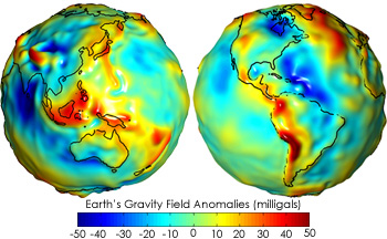
(image from https://earthobservatory.nasa.gov/features/GRACE/page3.php.) The measurement shown is the gravity “anomaly”, which is the deviation from the prediction for a smooth, uniform Earth. The unit of “milligal” is a unit of acceleration named after Galileo; one gal is equal to 0.01 m/s{}^2, which works out to about 1/1000 the size of g, so a milligal is 1/10^6 times g. Our estimated correction to g in Boulder of 0.05% of g works out to 500 milligals, so height is the dominant effect (and has clearly been subtracted to produce the shown anomaly map.)
Effective theory is a seemingly simple idea: basically an application of series expansion once again. But again, this is a really important idea in physics! Whenever we write down Newton’s laws, we’re also ignoring long-distance effects from things like the Sun’s gravitational field, and we’re ignoring quantum effects that will show up around atomic distance scales. So all of Newtonian physics is in fact an effective theory!
In fact, all of the “fundamental” forces are effective theories too, as far as we know. A famous example is gravity itself; if we try to calculate using the theory of gravity on scales where quantum mechanics is also important, then we find that the resulting effective theory diverges badly if we even ask theoretical questions about distances close to \ell_P, the Planck length I mentioned above. This is such an enormously short distance scale that we have no experiments that can possibly probe it, so far - but effective theory gives us a tantalizing hint that gravity has to change somehow if we can start to look at those really short distances.
5.3.2 Dark matter
The story of dark matter begins with a really simple physics question: how do we know the mass of the Sun M_{\odot}? I mentioned before that for the Earth, there’s only one reliable measurement of its mass, which is using the force of gravity exerted by the Earth. We can do the same for the Sun, by looking at the Earth’s orbit.
The force on the Sun due to the Earth is \vec{F}_g = -\frac{GM_{\odot} M_E}{R_{ES}^2} Now, the orbit of the Earth isn’t perfectly circular, but it’s pretty close; if we assume that it is circular, then this is also a centripetal force: \vec{F}_g = \vec{F}_c \Rightarrow \frac{GM_{\odot} M_E}{R_{ES}^2} = \frac{M_E v_E^2}{R_{ES}} or solving for the mass of the Sun, M_{\odot} = \frac{v_E^2 R_{ES}}{G}.
Finding the speed of the Earth’s orbit is easy: we know it completes a full orbit in 1 year, or 365.25 days. A full orbit is a change in angle of 2\pi, so the Earth’s angular speed is \omega_E = \frac{2\pi}{365.25\ {\textrm{days}}} \approx 2.0 \times 10^{-7} / s. Since v_E = \omega_E R_{ES}, we now know v_E in terms of R_{ES}. Determining the latter is actually tricky, although there are estimates dating back as much as 2300 years ago; I won’t go into details, but it involves geometric arguments with the Sun, Earth, and another astronomical body making a triangle. The advent of radar ranging to other planets can be combined with modern versions of these geometric calculations to yield a fairly accurate result, which I already quoted above: R_{ES} \approx 1.48 \times 10^{11} m.
Putting things together, we find M_{\odot} = \frac{\omega_E^2 R_{ES}^3}{G} = 1.9 \times 10^{30}\ {\textrm{kg}}.
For the Sun, we actually have a second way to estimate its mass: based on its size and density. Again using geometry, the radius of the Sun itself can be determined to be R_{\odot} = 7.0 \times 10^5 km. Thus, the mass will be related to the density as M_{\odot} = \rho_{\odot} V_{\odot} = \frac{4}{3} \pi R_{\odot}^3 \rho_{\odot}. We can estimate the density of the Sun because we know what it’s made of: primarily hydrogen and helium, heated into a superhot plasma. Now, this is definitely not a simple exercise: the temperature will have significant effects on the density, and so will the additional pressure generated by the huge gravitational pull of the Sun. But we have fairly complete models of the Sun’s interior, and it’s certainly possible to do the calculation carefully and get an estimate - see here for a taste of how such models work - of about 1400 kg/{\textrm{m}}^3. This once again gives a result of M_{\odot} \sim 2 \times 10^{30} kg.
This is a nice consistency check between our model of gravity and our model of the Sun. It also suggests a similar approach to a much more ambitious question: how much mass is in a galaxy like the Milky Way? The second method for weighing a galaxy is straightforward: you estimate how many stars there are, multiply by the mass of an average star (very roughly the mass of the Sun, but there are detailed models of stellar populations that can improve this!), and that gives you one version of M_{\textrm{galaxy}}.
The gravitational way of estimating a galaxy’s mass turns out to be a bit more involved. But we have a lot of extra information: since we can infer the motion of all of the visible stars in a galaxy, we can see “inside” the galaxy to probe its complete gravity field instead of having to rely only on objects well outside the galaxy, as we did for the Earth-Sun case.
Let’s restrict our attention to a certain fairly common kind of galaxy known as an elliptical galaxy, which can be nearly spherical - in fact, let’s assume it is spherical for the sake of our calculation. (I’ll comment on this assumption later.)
To find the gravitational field, we need to consider another variant of the sphere problem: finding the field inside of a solid sphere. We can set this up simply using Gauss’s law. Let’s take a sphere of radius R and consider r < R as shown:
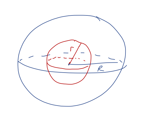
Using the result from the tutorial, the gravitational field inside the sphere is g(r) = -\frac{4}{3}\pi G \rho r So the strength of the gravitational field actually increases with distance! We can’t observe the gravity field directly, just the motion of the stars, so we have one more step, to relate this to the speed. The main dynamics of a galaxy is not that different from our solar system: the stars follow orbits around the galactic center of mass. If we make the assumption of an approximately circular orbit, then the force of gravity must be equal to the centripetal force, |\vec{F}_g| = |\vec{F}_c| \\ m|\vec{g}(r)| = \frac{mv^2}{r} \\ \frac{4}{3} \pi G \rho r = \frac{v^2}{r} \\ v = \sqrt{\frac{4\pi G \rho}{3}} r.
We can measure v and r, and then extract the density \rho from this equation to find the galaxy mass. Of course, this is only true inside the sphere, or equivalently in the middle of the galaxy where the density really is more or less constant. But if we look at stars close to the edge of the galaxy, we can treat them as being just outside a sphere, and we have our previous result g(a) = -\frac{GM_{\textrm{enc}}}{r^2} for r > R. Relating to the speed in the same way as before, we have \frac{GM_{\textrm{enc}}}{r^2} = \frac{v^2}{r} \\ v = \sqrt{\frac{GM_{\textrm{enc}}}{r}}. So if we can get good observations of stars at the edge of a galaxy, we can just measure their speeds directly to determine the mass. Overall, if we look at all of the stars, if the density is constant out to the edge of the visible galaxy at R, we expect the profile of speed vs. distance to look like this:
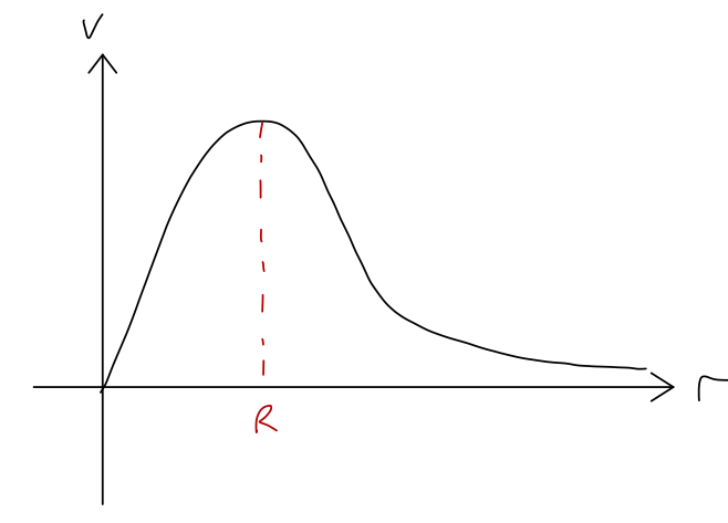
(Our prediction isn’t this smooth near R, but a smooth function is more realistic, due to measurement error and the fact that the density of a galaxy isn’t really uniform.) So far, so good. But what do we see if we actually do this experiment? Here is a plot of v vs. r for the galaxy NGC 3198: this is a spiral galaxy and not an elliptical, so I’m cheating a little; spirals seem to be easier to make this sort of observation of the full rotation curve in, probably because we get an unobstructed view of stars all the way to the center.
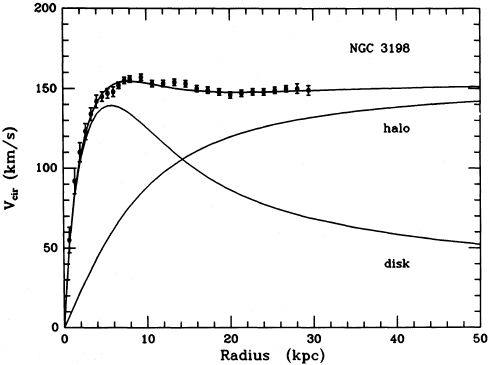
(from https://jila.colorado.edu/~ajsh/astr1200_18/dm.html, and originally https://ui.adsabs.harvard.edu/abs/1985ApJ…295..305V/abstract.)
The “disk” line shows the expected dependence; the data points show the observed results. You can see from the disk line that in this model, R for the galaxy is about 6 kpc (kilo-parsecs, a parsec is short for “parallax arcsecond” and is one of those somewhat arcane astronomy units; a parsec is about 3.3 light-years.) For small r the data agree well with the disk model, with speed increasing with distance, but then instead of the expected turnover, the velocity just becomes constant out to well beyond where the visible edge of the dense part of the galaxy is found!
One possibility is that we’ve neglected something: there is another force that we don’t know about, or our model of gravity is just wrong. This is still a possibility, although the preponderance of evidence is strongly in favor of the second option: dark matter. That is to say, what we have wrong isn’t the force law, but the density function: there must be some additional source of gravity that extends out beyond where the visible stars end. Quite far beyond, in fact; for most galaxies, a full explanation requires an enormous dark matter “halo” surrounding the visible galaxy:
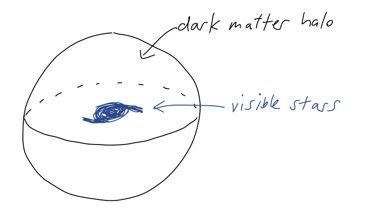
This has to be “dark” because it doesn’t emit or absorb light at all, or at best it does so very weakly; astronomical observations across the spectrum of light show nothing at all where the gravitational mass should be plentiful. This also brings me back to the comment about spherical galaxies: even for a spiral galaxy, the dark matter halo itself is still spherical (and much larger than the galaxy itself!), so our calculation still applies.
We can even guess what the density of the missing dark matter is using what we’ve derived so far: as you can see from the plot, the contribution to the speed from the halo goes roughly as \sqrt{r}. Working backwards, this requires a constant gravitational field, which in turn means that for the dark matter halo, \rho(r) \propto \frac{1}{r}. Of course, this is only one galaxy; there are other examples where v(r) becomes constant (which would require \rho(r) \propto 1/r^2) or begins to drop at very large distances. A commonly adopted model which works well for a large number of galaxies is the Navarro-Frenk-White profile, or NFW profile for short: \rho_{\textrm{NFW}}(r) = \frac{\rho_0}{(r/a)(1 + r^2/a^2)} introducing a second length scale a, the “scale radius”. This model can be argued as a simple but general parametrization of the behavior of so-called “cold and collisionless” dark matter - which can be tested using numerical simulations consisting of N masses only interacting through gravity.
Since it’s an active topic of research, I should say a little more about what we do know about dark matter. So far, the answer is “not very much”; experimental searches that attempt to capture the passing of a dark matter particle through an Earth-based detector have so far yielded nothing, except strong confirmation that it is indeed “dark” - any other interaction it has with ordinary matter must be very weak indeed.
However, we have a large amount of evidence for the gravitational effects of dark matter. In addition to observations of galactic structure (for which there are many examples):
- There is evidence for an imprint of dark matter on the cosmic microwave background, a uniform background noise that was formed in the very early universe.
- Over the very largest distance scales, the galaxies that make up our universe are not spread around randomly; instead, they seem to be organized into large, invisible filaments. This filamentary structure is consistent with simulations of the formation of the universe that include dark matter.
- Finally, according to the theory of general relativity (which replaces Newtonian gravity like special relativity replaces Newtonian mechanics), the path of a ray of light bends in a gravity field, an effect known as “gravitational lensing”. This is a complicated subject, but there are a number of observed examples where (for example) a distorted image of a distant galaxy is seen as its light passes near a closer galaxy. The mass of these lensing galaxies inferred from reconstructing the path of the light is consistent with the dark matter halo mass and not just the visible mass.
The story is not completely settled, of course; maybe a modification of gravity can account for all of the above, although since very different distances scales are involved it is quite difficult to formulate such a theory. The more likely explanation is that dark matter exists, and the hunt is on to discover what it is!