1 Space, time, and motion
1.1 Introduction
Mechanics is the study of motion, and motion is described using the spatial positions of a physical system as a function of time. So, the best place to start is by carefully defining how we will talk about space and time.
One warning Taylor (2005) gives that I’ll amplify: if my choices of notation are not what you’re used to, that’s a good thing! There are many conventions and notation choices out there; to read scientific books, papers, etc. more broadly, you need to get comfortable with changes to notation. In fact, there are some ways in which my notation will deviate from Taylor’s notation - I will be extra careful to call these differences out, however. I will also comment on popular alternatives in notation sometimes.
1.1.1 Units and dimensions
The foundation of science is reproducibility, which means if you and I do the same experiment, we will find the same results. But defining what “the same results” means requires us to agree on some ground rules. One very important detail is choice of units (look up the sad story of the Mars Climate Orbiter!), but you should be familiar with the basics of scientific units by now, so we’ll just agree to work in SI and move on.
Actually, one piece of terminology first: we will work in SI units, but a slightly more general concept than units is the idea of dimensions. A dimension is a basic physical property of some system. Meters, micrometers, feet, and light-years are all different units, but they all measure the same dimension, which is length. The important physical dimensions for mechanics are:
- Length (SI base unit: meters, m), [L] for short
- Time (SI base unit: seconds, s), [T] for short
- Mass (SI base unit: kilogram, kg), [M] for short
and in fact, that’s it: we can derive everything else. For example, energy (SI base unit: Joules, J) has dimensions of [M] \cdot [L]^2 / [T]^2, and correspondingly the Joule is equal to \textrm{J} = \textrm{kg} \cdot \textrm{m}^2 / \textrm{s}^2. As long as we only work in SI base units, we can use dimensions and units more or less interchangeably (and I will mix the terms together), but it’s worth remembering that there is a difference.
(Note: there are some other concepts that aren’t just simply derived from this set of three dimensions, like charge and temperature. But length, time, mass is all we will need for mechanics!)
The existence of dimensions gives a really important distinction between physics problems and pure math problems. The simple requirement of matching dimensions can greatly restrict the space of allowed solutions, and sometimes lets you guess the form of the right answer without a full solution (this is called dimensional analysis.) Even if you solve a problem in full, checking dimensions is a nice filter to easily verify your results (this will save you hours of confusion and many mistakes over the course of your physics career!)
Here, you should complete Tutorial 1A on “Math and Modeling.” (Tutorials are not included with these lecture notes; if you’re in the class, you will find them on Canvas.)
1.2 Vectors and coordinate systems
Having settled on units, we next have to agree on a coordinate system to describe where things are in our experiments. We live in three dimensions, so we need three coordinates - three numbers - to uniquely describe a given point in space. (You can take this as a definition of what “three dimensions” means, in fact.) We also need to agree on an origin, O, from which our coordinates are measured.
All of the below should be review at least partly, but it will be a good opportunity to refresh your memory and let me set up some math notation, for which I’ll generally try to follow Taylor. In addition to the coordinate definitions themselves, we’ll also be considering how vectors change as we change coordinates. (Vectors are essential to most of the physics we’ll study in this class!)
We also have to agree on our time coordinates, but since there’s only one dimension of time, that’s easy: if my time axis is t and yours is t', the only possible difference is that we might disagree on the origin, i.e. my t=0 s might be your t'=2 s. Unless explicitly said otherwise, I’ll assume that we always have a single common time axis t with common origin, and just worry about the other coordinates.
1.2.1 Rectangular coordinates
Let’s start with the most familiar coordinate system, called rectangular or sometimes rectilinear or Cartesian coordinates. These are the coordinates (x,y,z) that describe distances along a set of three perpendicular axes. Any choice of three axes will do, as long as they’re all mutually perpendicular!
At this point, it’s good to introduce vector notation, which will be very helpful in thinking about relating different coordinate systems. We define three unit vectors \hat{x}, \hat{y}, \hat{z} which point along the corresponding axes. Then we can write any other vector in terms of the unit vectors. For example, the position vector \vec{r} describes the location of an object relative to the origin:
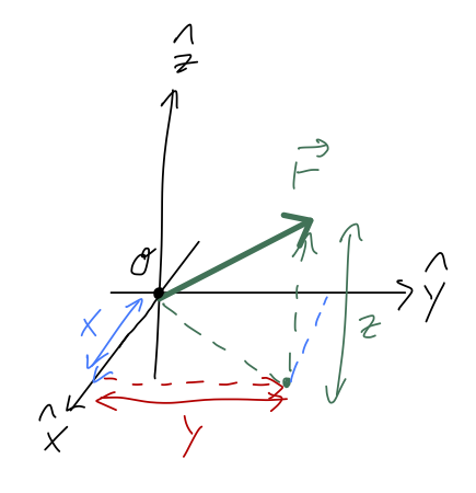
\vec{r} = x \hat{x} + y \hat{y} + z \hat{z} \tag{1.1}
Common alternative names for the unit vectors are \hat{i}, \hat{j}, \hat{k} and \hat{e}_1, \hat{e}_2, \hat{e}_3; the latter generic-looking set are sometimes used to describe other coordinate systems, so beware!
(Note on notation: I will use arrows to denote vectors; Taylor uses bold-face, so he would write the vector above as \mathbf{r}. Bold-face looks clean but arrow notation is much more practical when writing by hand!)
As mentioned above, keeping track of units is very important, so when we introduce new things I’ll try to mention their dimensions as well. Since \vec{r} has units of distance, and so do the individual lengths x,y,z, we notice that the unit vectors themselves have no units - they just point in a direction.
When we want to refer to components of a vector by name, we’ll use a subscript equal to the corresponding unit vector: for example, if \vec{v} is a velocity, then v_x is the speed in the x-direction. For the position vector, we have r_x = x.
1.2.2 The dot product
Vector information about an object and its motion is great, but often we want to know things like: “what is the speed of my object?” or “how far are these two masses from each other?” Speed and distance are examples of scalar information: they are quantities that don’t care about direction, which means they definitely aren’t vectors!
One useful way to get scalar information from vector information is the dot product, which multiplies two vectors together component by component and gives back a number: \vec{a} \cdot \vec{b} = a_x b_x + a_y b_y + a_z b_z. \tag{1.2}
We can immediately use this to define useful things. For example, the dot product of a vector with itself gives us the square of its length, just by the Pythagorean theorem: |\vec{r}| = \sqrt{ x^2 + y^2 + z^2} = \sqrt{\vec{r} \cdot \vec{r}} \tag{1.3} where paired vertical lines |...| gives absolute value for a regular number, but length for a vector. They’re sort of the same thing, because a vector’s length can’t be negative, and it’s easy to show that |-\vec{r}| = |\vec{r}|. When it isn’t ambiguous, I’ll usually write this simply as r = |\vec{r}|.
In general, if you go look up some trigonometry formulas, it’s not too hard to show that \vec{a} \cdot \vec{b} = ab \cos \theta, \tag{1.4} where \theta is the angle between the two vectors. I won’t derive this formula, but I will apply one other concept that I’ll emphasize over and over, which is checking limits and special cases (another technique to save you from hours of frustration!) First special case: if \vec{b} = \vec{a}, then the angle \theta is obviously zero, and we recover the formula \vec{a} \cdot \vec{a} = |\vec{a}|^2 from above. Our check is successful!
Another interesting limit is when \theta = 90^\circ: the formula tells us that the dot product should be ab \cos 90^\circ = 0. If we pick our coordinates axes so that \vec{a} = a \hat{x} and \vec{b} = b \hat{y}, for example, then it’s easy to confirm this from the definition. So this check passes too.
A natural question you might ask is: what if I’ve already picked my coordinate axes, and my vectors \vec{a} and \vec{b} aren’t along the coordinate axes? Why does the argument above still work? A really important point to remember is that vectors exist independent of our choice of coordinates. Mathematically, this is true by definition: obviously in physics, it had better be true, because a block sliding down a ramp only has a single velocity vector even if you and I measure it differently.
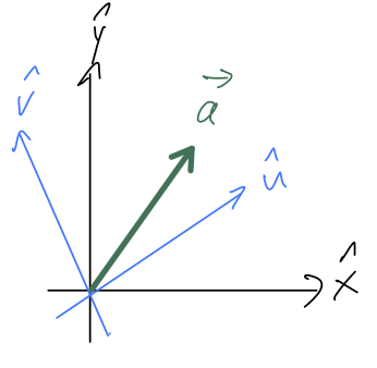
Since \vec{a} \cdot \vec{b} only depends on the vectors and not on any components, it is coordinate-independent. This is why I was allowed to pick my coordinates above to work out what happens to the dot product when \theta = 90^\circ.
A scalar quantity, like the distance between two objects, is independent of coordinate system. A vector quantity, like the velocity of an object, also exists independent of coordinate choices! However, the components of a vector will change when we change coordinates.
We emphasized that unit vectors like \hat{x} just point in a direction: they carry no units and their length doesn’t change. Using the dot product, we can define a unit vector pointing in the direction of any vector by dividing its length out: \hat{a} = \frac{1}{\sqrt{(\vec{a} \cdot \vec{a})}} \vec{a}. \tag{1.5} or using our informal notation for the length and inverting, \vec{a} = a \hat{a}. As another example, we can write the position vector as \vec{r} = r \hat{r}.
One more useful feature of the dot product is that we can use it to project out components. For example, the x component of an arbitary vector \vec{v} is given by: v_x = \vec{v} \cdot \hat{x} and similarly for v_y and v_z. This might seem kind of trivial if we already know what \vec{v} looks like in rectangular coordinates - but this simple observation is often useful if we’re changing coordinate systems.
The other important vector product to know is the cross product, \vec{a} \times \vec{b}. However, it will be a while until we actually have a use for it this semester, so I’ll defer talking about it until later on.
1.2.3 Cylindrical coordinates
Let’s do cylindrical coordinates next, because they only swap out two out of three coordinates from Cartesian coordinates: \hat{z} is kept the same. Ignoring the z-direction, we want to swap out the other two coordinates (x,y) for 2-d polar coordinates:
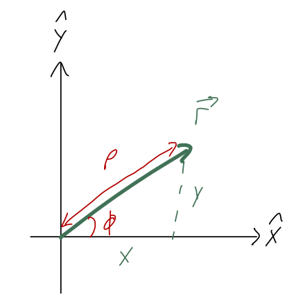
Taylor does something I think is confusing, which is to use r instead of \rho if he’s in two dimensions. I’ll always use \rho for the polar radius, keeping r for the three-dimensional position vector, i.e. distance to the origin.
(The symbol \rho we use for the distance to the origin is the greek letter “rho”. Greek letters are commonly used for variables in math and physics; here is a complete list on Wikipedia.) As we can read off the sketch, the relationship between the coordinates is x = \rho \cos \phi \\ y = \rho \sin \phi or going backwards, \rho = \sqrt{x^2 + y^2} \\ \tan \phi = \frac{y}{x}.
A word of warning about this last formula: you might be tempted to just use an inverse function to “simplify” it and write \phi = \tan^{-1} (y/x). The problem with this will be obvious if we plot the \tan^{-1} function:
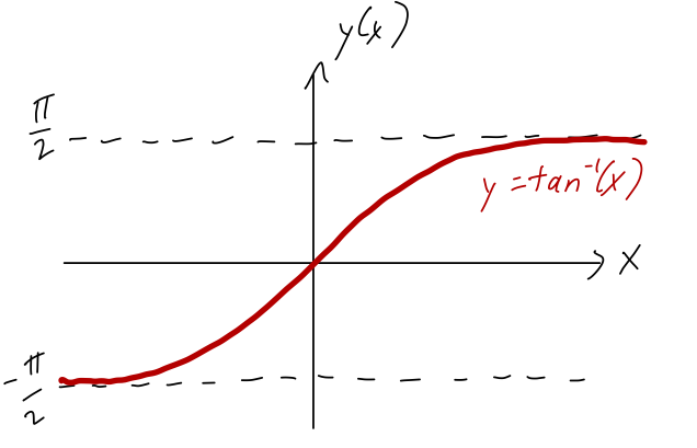
The range of \tan^{-1}, i.e. its set of possible output values, is (-\pi/2, \pi/2). But this only covers half of the plane! The issue is that if we reflect a point from (x,y) \rightarrow (-x,-y), the value of the ratio y/x doesn’t change: in terms of angles, \tan (\phi + \pi) = \tan \phi. So if you use the ratio y/x to find what the coordinate \phi is, double-check what quadrant your point is supposed to be in!
If you’re doing this numerically, it’s not hard to write a computer program that will use \tan^{-1} and then check the signs and add \pi if needed. However, the program needs to know both x and y separately. In Mathematica, if you give two numbers i.e. ArcTan[x,y], it gives you exactly this corrected result for \phi. In other programming languages, the ‘quadrant-aware’ version of the function is usually called arctan2.
If we want to do integrals in cylindrical coordinates, we need the volume element:
dV = \rho\ d\rho\ d\phi\ dz. \tag{1.6}
A tip to help remember this formula is to think about checking units. The units of volume are [L]^3, but the angle \phi is dimensionless, so if you just write out d\rho d\phi dz you should notice that you’re missing a unit of length - which comes from the extra factor of \rho.
One important note about volume elements, since I like to emphasize both geometric and algebraic solutions. We know that the Cartesian volume element is dV = dx dy dz, so maybe another way to derive this formula is to just use the coordinate change formulas above. If you try this, you’ll find that it doesn’t work! The problem is that when we’re computing a volume element, we have to account for the directions of the unit vectors; in Cartesian coordinates the element is just a cube, but in other coordinate systems we get a different shape. The correct general formula is actually the triple product dV = (\vec{dx} \times \vec{dy}) \cdot \vec{dz}. Since all of the axes are perpendicular in Cartesian coordinates, this just becomes simply dx dy dz. But in the current example, the difference matters; if you keep track of things properly, using this formula as the starting point should yield the correct cylindrical dV.
On to the unit vectors. Remember that the idea of a coordinate unit vector is that it points in the direction in which that coordinate increases; if we pick a point and sketch the polar coordinates on, it should be easy to see geometrically which way \hat{\rho} and \hat{\phi} point. But now, if we choose two different points and identify \hat{\rho} and \hat{\phi}, it’s easy to see that we have a new complication: the directions \hat{\rho} and \hat{\phi} depend on what point we are asking about!
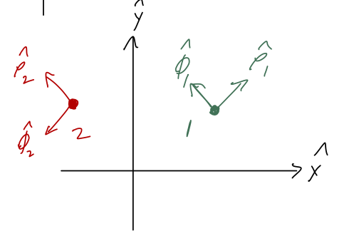
We can do a bit of trigonometry on any given point and easily show the general relationship \hat{\rho} = \cos \phi \hat{x} + \sin \phi \hat{y} \\ \hat{\phi} = -\sin \phi \hat{x} + \cos \phi \hat{y} The way in which they depend on our coordinates isn’t so bad: their directions just change with the angle \hat{\phi}.
Instead of going through the geometry, I’ll show you an algebraic way to derive the unit vectors instead. When we take the derivative of a vector \vec{v} with respect to some other variable s, the new vector d\vec{v}/ds gives us both the rate and the direction of change with respect to s. So when we say “the \rho direction”, what we mean is the direction of the vector d\vec{r}/d\rho. Recalling that we can rescale any vector to a unit vector by dividing its length out, we have the equations: \hat{\rho} = \frac{d\vec{r}/d\rho}{|d\vec{r}/d\rho|} \\ \hat{\phi} = \frac{d\vec{r}/d\phi}{|d\vec{r}/d\phi|}
We start by writing \vec{r} out in Cartesian components:
\vec{r} = x\hat{x} + y\hat{y} + z\hat{z}
Next, we substitute in the formulas for x and y in terms of cylindrical coordinates: \vec{r} = \rho \cos \phi \hat{x} + \rho \sin \phi \hat{y} + z\hat{z}
Now we can take derivatives, remembering that the derivative of a vector is still a vector: \frac{d\vec{r}}{d\rho} = \cos \phi \hat{x} + \sin \phi \hat{y} and \frac{d\vec{r}}{d\phi} = -\rho \sin \phi \hat{x} + \rho \cos \phi \hat{y}
These are the correct directions for \hat{\rho} and \hat{\phi} already; to make them unit vectors, we just have to normalize. It’s easy to show that d\vec{r}/d\rho is already a unit vector, while the length of the other vector is \left| \frac{d\vec{r}}{d\phi} \right| = \sqrt{\rho^2 (\sin^2 \phi + \cos^2\phi)} = \rho. So finally, we have \hat{\rho} = \frac{d\vec{r}/d\rho}{|d\vec{r}/d\rho|} = \cos \phi \hat{x} + \sin \phi \hat{y} \tag{1.7} \hat{\phi} = \frac{d\vec{r}/d\phi}{|d\vec{r}/d\phi|} = -\sin \phi \hat{x} + \cos \phi \hat{y} \tag{1.8}
matching the result above.
Let’s get a bit of practice with using these cylindrical unit vectors.
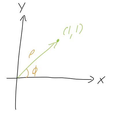
For the point (x,y) = (1,1), what is the position vector \vec{r} in terms of cylindrical unit vectors?
Answer:
The simplest way to understand this is by drawing the unit vectors on the sketch. You can do this just by geometric reasoning (the directions that \rho and \phi increase), or use our formulas above to find \hat{\rho} = \frac{1}{\sqrt{2}} (\hat{x} + \hat{y}) \hat{\phi} = \frac{1}{\sqrt{2}} (-\hat{x} + \hat{y}) with either method leading to the following diagram:
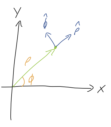
We see that \vec{r} is pointing directly along the \hat{\rho} direction, so it has no \hat{\phi} component. The length of the vector is \sqrt{2}, so we have simply \vec{r} = \sqrt{2} \hat{\rho}.
Notice that if we pick any point in the plane, the vector \vec{r} never has any \hat{\phi} component! This means that, for example, all of the points on the circle of radius \sqrt{2} from the origin have the same position vector \vec{r} = \sqrt{2} \hat{\rho}. The angular dependence is hidden within \hat{\rho} itself.
As the exercise above strongly hints, it’s easy to show that the general expression for the position vector in cylindrical coordinates is \vec{r} = \rho \hat{\rho} + z \hat{z} \tag{1.9}
with no \hat{\phi} component! If you are ever tempted to add a \phi \hat{\phi} term, you should be stopped by noticing it has the wrong units; \vec{r} should have units of distance, but \phi is unitless and so is \hat{\phi}, so something is wrong with \phi \hat{\phi}.
It’s also very important to point out that in cylindrical coordinates, the decomposition of a vector depends on what point it starts at. If we took the same vector \hat{x} + \hat{y} and started it at the point (1,-1), now it is pointing purely in the \hat{\phi} direction! We’ll mostly be dealing with vectors from the origin like \vec{r}, in which case this won’t be an issue, but I wanted to point it out anyway so you’re aware.
1.2.4 Time derivatives and unit vectors
As we’ve just emphasized, a key conceptual difference that appears in cylindrical coordinates vs. rectangular coordinates is that the unit vectors depend on what point we are looking at. This is very easy to see just by drawing two different vectors \vec{r}_1 and \vec{r}_2, and noting the directions of the unit vectors:
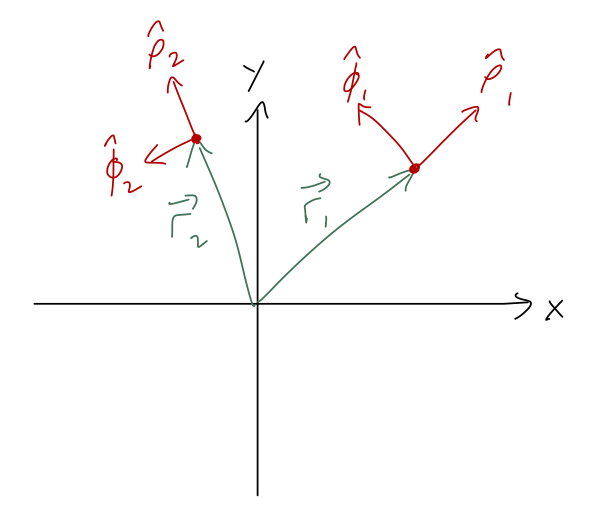
Looking forward to the physics a bit, in the context of mechanics \vec{r}_2 might represent a time-evolved version of \vec{r}_1 for some physical system, i.e. \vec{r}_1 = \vec{r}(t_1) and \vec{r}_2 = \vec{r}(t_2). If so, then it’s obvious that the unit vectors \hat{\rho} and \hat{\phi} themselves must be time-dependent.
Here I introduce some new notation, since we’ll be taking lots and lots of time derivatives: a dot over a quantity indicates acting on it with d/dt, \dot{q} \equiv \frac{dq}{dt}.
(Bonus notation: triple equals \equiv is the equivalence symbol and means “is defined to be”.) This applies both to scalars and vectors, so for example we can write \vec{v} = \dot{\vec{r}}. Finally, multiple dots can be used for multiple derivatives, so \ddot{q} = \frac{d^2 q}{dt^2}.
If you look at Taylor, he’ll give you a nice geometric argument for the time derivatives, with the result:
\dot{\vec{r}} = \dot{\rho} \hat{\rho} + \rho \dot{\phi} \hat{\phi}. \tag{1.10}
Instead of repeating his argument, let’s check the results using some limits. If \phi is constant, then \dot{\phi} = 0 and the velocity vector just reduces to one-dimensional speed in the \hat{\rho} direction, which makes sense. On the other hand, if \dot{\rho} = 0, then we are dealing with perfectly circular motion; in this case, we can recognize |\dot{\vec{r}}| = \rho \dot{\phi} as the standard expression relating tangential speed to angular speed (it might look more familiar if we write it instead as v = R \omega.)
We can also use algebra to find the same result. Recalling Equation 1.7 and taking the time derivative explicitly, we find that \frac{d\hat{\rho}}{dt} = -\dot{\phi} \sin \phi \hat{x} + \dot{\phi} \cos \phi \hat{y} \\ = \dot{\phi} \hat{\phi}, recognizing the form of the other unit vector from Equation 1.8 and substituting it back in. Then from Equation 1.9, we can see that (ignoring the \hat{z} component) the first derivative of the position vector is, by the product rule, \dot{\vec{r}} = \dot{\rho} \hat{\rho} + \rho \frac{d\hat{\rho}}{dt} and plugging in gives us back the result Equation 1.10.
Here, you should complete Tutorial 1B on “Time derivatives of the position vector”. (Tutorials are not included with these lecture notes; if you’re in the class, you will find them on Canvas.)
As explored in the tutorial, the other unit-vector derivative d\hat{\phi} / dt is crucial for finding the second derivative of the position vector, \ddot{\vec{r}} (also known as the acceleration - this will be very important when we start doing physics with these math results!) Let’s finish the derivation here, going slowly: \ddot{\vec{r}} = \frac{d^2 \vec{r}}{dt^2} = \frac{d}{dt} \left( \dot{\rho} \hat{\rho} + \rho \dot{\phi} \hat{\phi} \right) \\ = \ddot{\rho} \hat{\rho} + \dot{\rho} \frac{d\hat{\rho}}{dt} + (\dot{\rho} \dot{\phi} + \rho \ddot{\phi}) \hat{\phi} + \rho \dot{\phi} \frac{d\hat{\phi}}{dt} \\ = \ddot{\rho} \hat{\rho} + \dot{\rho} \dot{\phi} \hat{\phi} + (\dot{\rho} \dot{\phi} + \rho \ddot{\phi}) \hat{\phi} - \rho \dot{\phi}^2 \hat{\rho}
\Rightarrow \ddot{\vec{r}} = (\ddot{\rho} - \rho \dot{\phi}^2) \hat{\rho} + (\rho \ddot{\phi} + 2 \dot{\rho} \dot{\phi}) \hat{\phi}. \tag{1.11}
Right now this isn’t a very illuminating result; we’ll come back to it below in the context of Newton’s laws and motion.
1.2.5 Spherical coordinates
In spherical coordinates, we adopt r itself as one of our coordinates, in combination with two angles that let us rotate around to any point in space. We keep the angle \phi in the x-y plane, and add the angle \theta which is taken from the positive \hat{z}-axis:
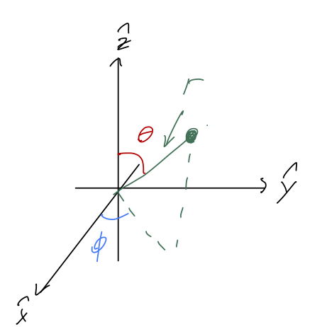
(Confusingly, \theta is usually called the “polar angle”, thinking of the z-axis as the “pole”. In this case, \phi is called the “azimuthal angle”. See Taylor (2005), p.135.)
Be aware that these are the physics conventions for what to call these angles. Mathematicians tend to prefer the opposite choice, using \theta as the azimuthal angle and \phi the polar. On top of the angle name confusion, math books (and some physics texts) will also use \rho for the spherical distance and r the polar distance. Be very careful when looking at other resources!
The relationship between spherical and cylindrical coordinates is actually relatively simple to work out, as we can see by looking at a cross-section containing both \vec{r} and \hat{z}:
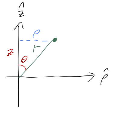
It’s easy to see from the sketch that z = r \cos \theta \\ \rho = r \sin \theta We can then take this and plug in one more step to get the formulas for rectangular coordinates: x = r \sin \theta \cos \phi \\ y = r \sin \theta \sin \phi \\ z = r \cos \theta If you forget exactly where the sine and cosines go in this expression, I find it’s easiest to think about converting from cylindrical coordinates. I’ll skip the derivation of the volume element since it’s more involved, but the result is important for doing integrals: dV = r^2 \sin \theta\ dr\ d\theta\ d\phi. \tag{1.12}
We could find results for the unit vectors in spherical coordinates \hat{r}, \hat{\theta}, \hat{\phi} in terms of the Cartesian unit vectors, but we’re not going to be doing vector calculus in these coordinates for a while, so I’ll put this off for now - it’s a bit messy compared to cylindrical. I will simply note that basically by definition, the decomposition of the position vector \vec{r} is extremely simple in spherical coordinates: \vec{r} = r \hat{r}. \tag{1.13}
1.3 Motion and Newton’s laws
Now that we’ve set up our coordinate system basics, let’s turn back to physics, starting with Newton’s laws of motion. Taylor discusses some fundamentals about defining mass and force, but I’ll let you read that on your own. Here, let’s just remind ourselves what the laws are:
- In the absence of forces, an object moves with constant velocity.
- An object of mass m subject to a net force will accelerate according to the relation \vec{F} = m \vec{a}.
- If object 1 exerts a force on object 2, there is an equal and opposite force exerts on object 2 by object 1,
\vec{F}_{12} = -\vec{F}_{21}.
In our modern understanding, the first law is more or less redundant, because the second law immediately tells us that if \vec{F} = 0, then \vec{a} = 0; since \vec{a} = d\vec{v}/dt, no acceleration means constant velocity. (This isn’t quite true, because you can think of the first law as something to check to make sure you’re in an inertial frame where the second law will hold; see the discussion in Taylor, chapter 1. This semester, we will do everything in inertial frames of reference - which just means we have to avoid situations in which our coordinate systems are tied to accelerating objects. (For a more detailed discussion of this topic, see the aside on reference frames below.)
We mentioned vector time derivatives before, but let’s talk a bit more about them, and define some terms. Taking the time derivative of the position vector \vec{r} gives us the velocity vector, \vec{v} = \frac{d\vec{r}}{dt}, and one more derivative gives us the acceleration vector, \vec{a} = \frac{d\vec{v}}{dt} = \frac{d^2 \vec{r}}{dt^2}. Thus, using dot notation to make things more compact, we can write Newton’s second law as \vec{F} = m\vec{a} = m\ddot{\vec{r}}. \tag{1.14}
1.3.1 Newton’s laws in rectangular coordinates
Let’s think about how this breaks into components, starting with rectangular coordinates. The velocity vector then becomes: \frac{d}{dt} \vec{r} = \frac{d}{dt} \left( x \hat{x} + y \hat{y} + z \hat{z} \right) \\ = \dot{x} \hat{x} + \dot{y} \hat{y} + \dot{z} \hat{z}. \tag{1.15} Taking another time derivative for acceleration will just give us double-dots instead of single-dots; again, the unit vectors don’t depend on time. So we have for Newton’s second law: F_x \hat{x} + F_y \hat{y} + F_z \hat{z} = m \left(\ddot{x} \hat{x} + \ddot{y} \hat{y} + \ddot{z} \hat{z} \right)
This is, in fact, just three separate copies of the same equation, one for each direction: F_x = m\ddot{x} \\ F_y = m\ddot{y} \\ F_z = m\ddot{z}
Our vector equation has split apart into a system of differential equations. These equations are collectively known as the equations of motion, because if we solve them, we know the answer for \vec{r}(t) - we know what the motion of the system will look like over time.
The equations of motion are the system of differential equations that we solve for any given problem in order to find \vec{r}(t). (If we know \vec{r}(t), then we know how our system’s position evolves with time - this is the motion!) This semester, the equations of motion will always come from Newton’s second law.
Before we even move on from rectangular coordinates, it’s important to note that we have a great deal of freedom in choice of coordinate system. For example, consider the motion of a block sliding down a ramp with friction:
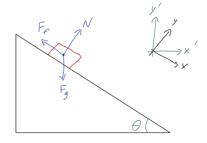
Taylor does this as example 1.1, in fact; if you look at his solution, he takes his x-axis to be parallel to the ramp and y-axis perpendicular to it, as pictured in the top right (the black coordinate axes.) But we could also work in the green coordinate system, where y' is in the direction of gravity instead. The choice is arbitrary - the physics is the same! Of course, the algebra might be easier if we pick our coordinates well, and in fact Taylor’s choice gives the simplest math if we follow the solution through.
(Just to make this point once again: notice that I have drawn two coordinate systems, but only one free-body diagram. The force vectors are the same in any coordinates, even if how we break them into components is different!)
You should already be familiar with solving simple problems using Newton’s laws and free-body diagrams! If you need a refresher, click to expand the bonus example below which contains the full solution in the primed coordinates.
We’ll treat this as a two-dimensional problem, as indicated, which just means that we ignore the z coordinate. (This is valid because of Newton’s first law: if there are no z-direction forces, then there is no interesting z-direction motion at all.)
To proceed, we’ll need to split all the forces into components. Let’s draw some angles on our free-body diagram:
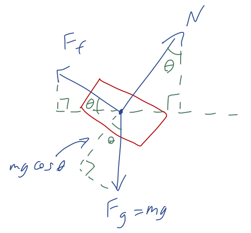
(if where I put the \theta’s in my diagram isn’t obvious to you, draw more parallel lines in and use right triangles to identify which angles are \theta and which are 90^\circ - \theta.) From the diagram, the forces split into components are, using the often-convenient notation that \vec{F} = (F_x, F_y):
\vec{N} = (N \sin \theta, N \cos \theta) \\ \vec{F}_f = (-F_f \cos \theta, F_f \sin \theta) \\ \vec{F}_g = (0, -mg)
Now, we know that the normal force N is equal and opposite to the magnitude of all other forces acting perpendicular to the surface of the ramp. From the diagram, we can just read off that it is equal to a component of the gravitational force, N = mg \cos \theta. The second fact we know is that the magnitude of the frictional force is proportional to the normal force, F_f = \mu N = \mu mg \cos \theta. Plugging back in, then, we have the net forces in the x' and y' directions: \vec{F}_{\textrm{net}} = \vec{N} + \vec{F}_f + \vec{F}_g \\ = \left(N \sin \theta - F_f \cos \theta \right) \hat{x}' + \left(N \cos \theta + F_f \sin \theta - mg \right) \hat{y}' \\ = mg \left( \cos \theta \sin \theta - \mu \cos^2 \theta \right) \hat{x}' + mg \left(\cos^2 \theta + \mu \cos \theta \sin \theta - 1 \right) \hat{y}'
This looks a little messy, but let’s keep going. Now that we have the net force, we can solve for the accelerations using \vec{F}_{\textrm{net}} = m \ddot{\vec{r}}, which gives us two equations looking at each component (and cancelling off the mass): \ddot{x}' = g \cos \theta (\sin \theta - \mu \cos \theta) \\ \ddot{y}' = -g (1 - \cos^2 \theta - \mu \sin \theta \cos \theta) \\ = -g \sin \theta (\sin \theta - \mu \cos \theta) where I’ve used a trig identity to simplify the last line; now the x' and y' equations look very similar.
The good news is that even though these still don’t look so nice, everything on the right-hand side of both equations is constant, so to solve for the motion, all we have to do is integrate twice, for example: \dot{x}'(t) = v_{x,0} + \int_0^{t} dt' \ddot{x}'(t') = v_{x',0} + gt \cos \theta (\sin \theta - \mu \cos \theta) \\ x'(t) = \int_0^t dt' \dot{x}'(t') = x'_0 + v_{x',0} t + \frac{1}{2} gt^2 \cos \theta (\sin \theta - \mu \cos \theta) and similarly, y'(t) = y'_0 + v_{y',0} t -\frac{1}{2} gt^2 \sin \theta (\sin \theta - \mu \cos \theta). If we assume starting from rest, then v_{x',0}, v_{y',0} are set to zero; if we also start at the origin, then x'_0 = y'_0 = 0 and we have our final result, shown below.
Solving for the motion in the primed coordinates gives the result (starting at rest from the origin): x'(t) = \frac{1}{2} gt^2 \cos \theta ( \sin \theta - \mu \cos \theta) \tag{1.16} y'(t) = -\frac{1}{2} gt^2 \sin \theta (\sin \theta - \mu \cos \theta). \tag{1.17}
Here \mu is the coefficient of kinetic friction for the moving block.
First, convince yourself that the units of the solution above make sense. Then show that if \theta \rightarrow 90^\circ, you get the expected result (freefall, since the ramp is now vertical.)
As a bonus, can you figure out why taking the other limit \theta \rightarrow 0^\circ appears to give nonsensical results? (Hint: think about both static and kinetic friction…)
Answer:
If \theta \rightarrow 90^\circ, then the ramp becomes completely vertical, so the motion should only be in the y' direction, and it should just be freefall. At 90^\circ we have \cos \theta = 0 and \sin \theta = 1, so x'(t) \xrightarrow{\theta = 90^\circ} x_0' + \frac{1}{2} gt^2 (0) (1 - 0\mu) = x_0' \\ y'(t) \xrightarrow{\theta = 90^\circ} y_0' - \frac{1}{2} gt^2 (1) (1 - 0\mu) = y_0' - \frac{1}{2} gt^2 so indeed, we have freefall in the y' direction and no motion in the x' direction.
How about the opposite limit, \theta \rightarrow 0^\circ? Since the motion is entirely caused by gravity, what we expect to find is that as the ramp becomes completely flat, all motion stops. Plugging in again, we find this time that x'(t) \xrightarrow{\theta = 0^\circ} x_0' + \frac{1}{2} gt^2 (1) (0 - 1\mu) = x_0' - \frac{1}{2} \mu gt^2 \\ y'(t) \xrightarrow{\theta = 0^\circ} y_0' - \frac{1}{2} gt^2 (0) (0 - 1\mu) = y_0'
The y'(t) result is fine, but our block will apparently start sliding backwards in the x' direction if the ramp is laid flat! What went wrong with our calculation?! (Think about it yourself, before you continue reading…)
In fact, our calculation above is just fine. The problem that was revealed when \theta \rightarrow 0^\circ has to do with our starting assumptions. In particular, we assumed a single coefficient of friction \mu. Since our block is in motion, this must be the coefficient of kinetic friction, \mu_k. However, we know that there is also a coefficent of static friction \mu_s that must be overcome if the block is starting at rest, F_{f,s} \leq \mu_s mg \cos \theta, which will keep the block from moving (i.e. give zero accelerations) if the other forces are not large enough. We can take the x'-direction net force and solve: F_{\textrm{net}, x'} = N \sin \theta - F_f \cos \theta = 0 \\ mg \cos \theta \sin \theta = F_f \cos \theta \\ mg \sin \theta \leq \mu_s mg \cos \theta \\ \tan \theta \leq \mu_s
So the full picture is: if the angle \theta is small enough that \tan \theta \leq \mu_s, then the block just won’t move at all. Since generally \mu_k \leq \mu_s, this means that \tan \theta \geq \mu_k whenever static friction is overcome; this means that the offending term which changed the sign of our x'-direction motion, (\sin \theta - \mu_k \cos \theta) \geq \sin \theta - \tan \theta \cos \theta \geq 0 and we don’t have any problems with backwards-moving blocks anymore.
Since the physics is the same, we should also be able to show that this answer matches the one Taylor finds in the unprimed coordinates. This is a simple exercise in trigonometry, or dot products, so I’ll leave it to you!
Apply a change of coordinates to the results above for x'(t) and y'(t), and show that you reproduce the answers given in Taylor (1.1) for x(t) and y(t).
Answer:
I’ll show you the answer for x(t) only below; it’s straightforward to follow the same steps for y(t) (and you know what you should find!)
Let’s put our knowledge of vector coordinate systems to use and work out the coordinate change. First, we add the angle \theta to our coordinate diagram:
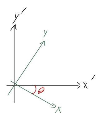
To see how the coordinate systems are related, let’s think in terms of the unit vectors. Using the formula Equation 1.4, we can easily see that \hat{x} \cdot \hat{x}' = \cos \theta and \hat{x} \cdot \hat{y}' = \cos (\theta + \frac{\pi}{2}) = -\sin \theta using a trig identity. You can convince yourself that the minus signs are correct by inspecting the diagram. Next, we take the position vector \vec{r} and decompose in both coordinate systems: \vec{r} = x \hat{x} + y\hat{y} = x' \hat{x}' + y' \hat{y}'. Observing that x = \hat{x} \cdot \vec{r} and using the dot products we just found on the right-hand side of the above equation, we immediately find that x(t) = x'(t) \cos \theta - y'(t) \sin \theta where I’ve put the time-dependence back to remind us that this relation is always true.
Putting our solutions together, then, we have x(t) = \cos \theta \left(\frac{1}{2} gt^2 \cos \theta (\sin \theta - \mu \cos \theta)\right) - \sin \theta \left( -\frac{1}{2} gt^2 \sin \theta (\sin \theta - \mu \cos \theta) \right) \\ = \frac{1}{2} gt^2 (\sin \theta - \mu \cos \theta) and if we open up the textbook, we’ll find that this matches Taylor’s solution exactly.
Note: this is an important concept - but also, hopefully one you have seen before. We won’t be making use of the explicit reference-frame notation introduced below at all this semester, which is why this is an aside and not part of the main lecture notes. If you want to know more about what “inertial frame” really means, read on!
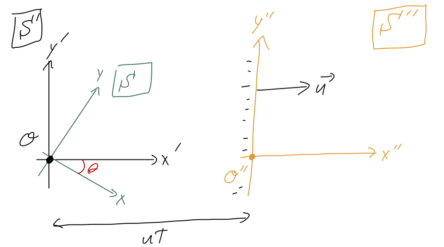
Whenever we do classical mechanics, we have to specify a reference frame. Reference frames are choices of coordinate systems, but because we’re dealing with both time AND space, they have an extra complication as compared to fixed coordinates: two frames can be moving relative to one another. Following Taylor, we’ll use a script \mathcal{S} to denote a reference frame. \mathcal{S} includes :
- A coordinate system,
- An origin \mathcal{O}, and finally
- Some specification of how \mathcal{O} is or isn’t moving, relative to some physical object or other point of reference.
Our chosen coordinates (x', y') for the ramp problem are an example of a reference frame \mathcal{S}'; Taylor’s rotated coordinates (x,y) are a different reference frame \mathcal{S}. Both frames have the same origin, and both are fixed with respect to the ramp, which means there’s also no relative motion between \mathcal{S} and \mathcal{S}'. However, we could come up with a third frame \mathcal{S}'' with coordinates (x'', y''), defined by the following relations: x''(t) = x'(t) - ut \\ y''(t) = y'(t) In other words, the origin of \mathcal{S}'' is moving horizontally to the right with constant speed u.
Since we already solved for the motion in \mathcal{S}', we can just use the coordinate change to find the motion in \mathcal{S}'':
x''(t) = x''_0 + (v_{x',0} - u) t + \frac{1}{2} gt^2 \cos \theta (\sin \theta - \mu \cos \theta) \\ y'(t) = y''_0 + v_{y',0} t -\frac{1}{2} gt^2 \sin \theta (\sin \theta - \mu \cos \theta). Notice that if our block starts at rest with respect to the ramp, it will appear to be moving to the left with initial speed u in our moving coordinates.
Just using a change of frame on our solution is always valid; if we have solved the equations of motion in one reference frame, we know the answer in any other frame. However, we have to be careful if we start in a given reference frame and try to apply Newton’s laws. If you try it in the \mathcal{S}'' frame, the forces will all be exactly the same, and you’ll find the same answer that we got above. However, when you have moving frames you have to be careful - Newton’s laws do not work (without modification) in accelerating frames! Accelerating frames are also called non-inertial frames, because the law of inertia (Newton’s first law) doesn’t hold - and neither does the second law.
We can explicitly see the breakdown of Newton’s laws if we try to use them in a very simple accelerating frame, provided by a moving elevator:
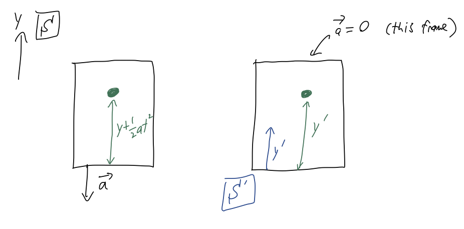
We drop a ball inside an elevator, from initial height y_0. From the point of view of frame \mathcal{S}, fixed with respect to the ground, the elevator is moving straight down with constant acceleration a. As pictured, we can define a second frame of reference \mathcal{S}' which is fixed to the elevator (so the point of view of an experimenter riding the elevator, basically.)
Let’s work out the motion in frame \mathcal{S} first. Neglecting air resistance, the only force acting on the ball is gravity: \vec{F}_g = -mg\hat{y} Using Newton’s second law, \vec{F}_{\textrm{net}} = -mg \hat{y} = m\vec{a} = m(\ddot{x} \hat{x} + \ddot{y} \hat{y}) so nothing happens in the \hat{x}-direction, but vertically we have a constant acceleration, \ddot{y} = -g. If we drop the ball at rest, integrating twice gives us y(t) = y_0 - \frac{1}{2} gt^2. So far, we haven’t mentioned the elevator at all; it enters in when we ask how far the ball is from the floor of the elevator at any given time. From the diagram, we can see right away that \Delta y(t) = y(t) + \frac{1}{2} at^2 = y_0 + \frac{1}{2} (a-g) t^2. In particular, notice that if the elevator is also free falling (a=g), then the ball will appear to be suspended above the floor.
What about the frame \mathcal{S}'? Well, the only force in the problem is still gravity, so we conclude right away that y'(t) = y'_0 - \frac{1}{2} gt^2. y'(t) is exactly the same thing as \Delta y(t), the distance from the floor to the ball. But we don’t see a anywhere, and in particular we don’t see any possibility for the ball to be suspended in mid-air. This is a contradiction!
Obviously, one of our answers is wrong, and if you remember the fine print on Newton’s laws, you may already know the answer: the calculation in \mathcal{S}' is wrong, because \mathcal{S}' is an accelerating (non-inertial) frame of reference.
The good news is that we’re never forced to use a non-inertial frame, because frames of reference are our choice! Our calculation in the frame of an observer outside the elevator is perfectly fine. But it’s an important point to be aware of.
1.3.2 Newton’s laws in cylindrical coordinates
Now that we’ve reviewed both Newton’s laws and curvilinear coordinate systems, let’s have a closer look at what happens when we put the two together. We’ll focus mainly on cylindrical coordinates, which will show the important features; spherical is more complicated but not really different.
Remember that one of the nice things about Newton’s laws in Cartesian coordinates is that they split apart into three separate equations for the x,y,z directions. Let’s remind ourselves why: Newton’s second law reads \vec{F} = m\ddot{\vec{r}} \\ F_x \hat{x} + F_y \hat{y} + F_z \hat{z} = m \frac{d^2}{dt^2} \left( x \hat{x} + y \hat{y} + z\hat{z} \right) and then acting with the time derivatives and matching components, we read off the individual equations F_x = m\ddot{x} and so on.
Now, we can do the same thing in cylindrical coordinates, using our results from above: F_\rho \hat{\rho} + F_\phi \hat{\phi} + F_z \hat{z} = m \frac{d^2}{dt^2} \left( \rho \hat{\rho} + z \hat{z} \right) You might be tempted to just starting matching terms again and conclude that F_\rho \stackrel{?}{=} m\ddot{\rho}. But there’s an immediate problem, which is that there doesn’t seem to be a \hat{\phi} term on the right-hand side! Does this mean that F_\phi is just irrelevant, no matter how large the force is? (That seems like a strange conclusion…)
The resolution to this problem is that the simple argument above is ignoring the time dependence of the cylindrical unit vectors. In fact, we already did the hard work above: Equation 1.11 contains the full result for \ddot{r} taking this into account properly. Plugging that result in, we have
F_\rho \hat{\rho} + F_\phi \hat{\phi} + F_z \hat{z} = m (\ddot{\rho} - \rho \dot{\phi}^2) \hat{\rho} + m(\rho \ddot{\phi} + 2 \dot{\rho} \dot{\phi}) \hat{\phi} + m \ddot{z} \hat{z}
from which we can read off the equations of motion: F_\rho = m(\ddot{\rho} - \rho \dot{\phi}^2) \tag{1.18} F_\phi = m(\rho \ddot{\phi} + 2\dot{\rho} \dot{\phi}) \tag{1.19} and F_z = m\ddot{z} as in rectangular coordinates.
The good news is that we now have dependence on all three coordinates, and on all three components of the force. The bad news is that this is going to give much more complicated differential equations for us to solve! (Attacking them directly for the most general problems, using the alternative Lagrangian formulation, is something you’ll come back to next semester.)
However, there are a number of specific problems where cylindrical coordinates are the best choice for solving using Newton’s laws.
Here, you should complete Tutorial 1C on “Motion in polar coordinates”. (Tutorials are not included with these lecture notes; if you’re in the class, you will find them on Canvas.)
Another good example of a problem best solved in cylindrical coordinates is a simple pendulum:
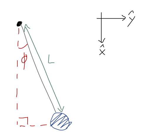
Note that I’ve turned the coordinates around a bit compared to how we usually draw them; this is so that I can identify the angle \phi = 0 with the lowest point of the pendulum. (Again, physical intution: we know that hanging straight down is a special point because the pendulum won’t move if we start it there. So we anticipate the answer will be a bit simpler with these coordinates.)
Once again, the full setup and solution for the pendulum is included as a bonus example below; we won’t go through it in lecture. But I will go through the start, to make a point. We should begin with a free-body diagram:

Let’s draw angles onto our free-body diagram and identify the unit-vector directions in cylindrical coordinates:
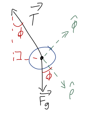
We immediately see that \hat{\phi} is perpendicular to T, which means that T_\phi is zero! This is one of the nice things about using cylindrical coordinates for this problem, the fact that the vector expression for tension is always the same, \vec{T} = -T \hat{\rho}, regardless of where the pendulum is. This is the payoff of using cylindrical coordinates; it makes our force equations “nicer”!
In lecture I will skip to the answer at this point, but if you want some practice you can click to go though the bonus example in detail.
For the pendulum, the cylindrical radius is fixed to the length of the string, \rho = L. This means that time derivatives of \rho vanish, leaving us with the equations F_\rho = -mL \dot{\phi}^2 \\ F_\phi = mL \ddot{\phi}
Notice, by the way, that if we were studying purely circular motion (e.g. the pendulum is being spun around on a flat surface instead of hanging vertically), we would have \dot{\phi} = v/L, and the first equation becomes F_\rho = -mL \left( \frac{v}{L} \right)^2 = -m\frac{v^2}{L}
which is the familiar equation for centripetal force. (By assumption of circular motion, the angular speed \dot{\phi} is constant, so the second equation is just F_\phi = 0.)
Back to the more general case of a pendulum.
As for gravity, we will need to decompose it into radial and tangential pieces. This time I’ll do it the geometric way, but note that you can also start with F_g = -mg\hat{y} and use algebra as an alternative way to convert. (Try it out if you’re not comfortable with vector algebra yet!) From the sketch above, we readily find that \vec{F}_g = mg \cos \phi \hat{\rho} - mg \sin \phi \hat{\phi}
Now we can plug back in to Newton’s laws in cylindrical components. Combining the radial forces, the first equation reads mg \cos \phi - T = -mL \dot{\phi}^2 and the second is -mg \sin \phi = mL \ddot{\phi}.
To solve for the motion, we can completely ignore the first equation, because it contains the unknown tension force T. (If we care about the tension, like if we know our string has a max tension and we want to predict whether it will break, we can go back and check at the end once we know \phi(t).) The second equation simplifies to the final result given below.
The results of the example calculation above are a single equation of motion for the angle \phi of the pendulum: \ddot{\phi} = -\frac{g}{L} \sin \phi.
Let’s check units, always a good practice: \phi is dimensionless, g has units of m/s^2, and L has units of m, so we have 1/s^2 on the right. This matches the left exactly, because d/dt itself has units of 1/s. (If this isn’t clear to you, think about the basic definition of a derivative: du/dt comes from the infinitesmal limit of \Delta u / \Delta t, and the units of \Delta t are clearly the same as the units of t.)
In this case both sides depend on the unknown \phi, so we can’t just integrate with respect to time. In fact, this is actually a surprisingly hard differential equation to solve, for such a simple system! There is no analytic solution in terms of elementary functions in general, but we can find an approximate solution: if we assume the angle \phi is always small (the ‘small-angle approximation’), then we can Taylor expand the right-hand side about \phi=0, \sin \phi \approx \phi\ + ... giving the simpler equation \ddot{\phi} = -\frac{g}{L} \phi. This still depends on \phi on both sides, but it has a relatively simple general solution, of the form \phi(t) = A \sin (\omega t) + B \cos (\omega t) where \omega = \sqrt{g/L}. At this point, we’re not ready to study how to get that general solution yet, but it’s easy for you to plug it back in and check that it works.
We’re starting to see that there are examples of equations of motion where the forces depend on coordinates, and we can’t just solve by simply integrating. In fact, this is a great point for us to go back to math, and start to study the more general theory of differential equations.
1.4 Ordinary differential equations
As we’ve started to see, solving equations of motion in general requires the ability to deal with more general classes of differential equations than the simple examples from first-year physics. Before we go back to mechanics, let’s start to think about the general theory of differential equations and how to solve them.
Specifically, we’ll begin with the theory of ordinary differential equations, or “ODEs”. The opposite of ordinary is a partial differential equation, or “PDE”, which contains partial derivatives; an ordinary DE has only regular (total) derivatives, or in other words, all of the derivatives are with respect to one and only one variable. Newtonian mechanics problems are always ODEs, because we only have derivatives with respect to time in the second law.
Now, a very important fact about differential equations is that their solutions alone are not unique; we need more information to find a complete solution. As a simple example, consider the equation \frac{dy}{dx} = 2x You can probably guess right away that the function y(x) = x^2 satisfies this equation. But so does y(x) = x^2 + 1, and y(x) = x^2 - 4, and so on! In fact, this equation is simple enough that we can integrate both sides to solve it: \int dx \frac{dy}{dx} = \int dx 2x \\ y(x) = x^2 + C remembering to include the arbitrary constant of integration for these indefinite integrals. So the equation alone is not enough to give us a unique solution. But in order to fix the constant C, we just need a single extra piece of information. For example, if we add the condition y(0) = 1 then y(x) = x^2 + 1 is the only function that will work.
Now that we’re going to be writing a lot of integrals, a brief comment on integral notation to avoid some common confusion. In mathematics, the most common convention for integrals is that the differential which indicates what variable we are integrating over is at the end:
\int x^2 dx = \frac{1}{3} x^3
This lets you easily and clearly do things like mixing indefinite integrals with other functions of f: \int x^2 dx + \frac{2}{3} x^3 = x^3.
On the other hand, in physics a more common convention (and the one we will use!) is to put the differential at the start of the integral, next to the integral sign: \int dx\ x^2 = \frac{1}{3} x^3.
This will make writing the second equation above look ambiguous, but I can fix that by using parentheses/brackets: \int dx\ \left( x^2 \right) + \frac{2}{3} x^3 = x^3.
This seems obviously worse, and it is, but in physics we rarely write equations like this! Typically when we integrate over a variable, it will be a definite integral and that variable won’t appear in the resulting equation. We also do a lot more multi-dimensional integrals, where I would say the physics notation has a nice advantage - it shows clearly which integral is using which variable: compare \int_0^1 \int_0^3 \int_{-1}^{1} \sqrt{x^2 + y^2 + z^2} dx dy dz (math convention) with \int_0^1 dz \int_0^3 dy \int_{-1}^{1} dx \sqrt{x^2 + y^2 + z^2} (physics convention), I think the second one is much clearer!
What if we have a second-order derivative to deal with, like in Newton’s second law \vec{F} = m \ddot{\vec{r}}? To solve this equation (or indeed any ODE that has a second-order derivative), we will need two conditions to find a unique solution. One way to think of this is to think about solving the equation by integration; to reverse both derivatives on d^2 \vec{r} / dt^2, we have to integrate twice, getting two constants of integration to deal with.
This statement turns out to be true in general, even though we can’t solve most ODEs just by integrating directly: every derivative that has to be reversed gives us one new unknown constant of integration. Notice that I’ve been using a calculus vocabulary term, which is ‘order’: the object \frac{d^{(n)} f}{dx^n} = \left( \frac{d}{dx} \right)^n f(x) is called the n-th order derivative of f with respect to x. The same vocabulary term applies to ODEs: the order of an ODE is equal to the highest derivative order that appears in it. (So Newton’s second law is a second-order ODE; to solve it we need two conditions, usually the initial position and initial velocity.)
Here’s another way to understand how order relates to the number of conditions. Using Newton’s law as an example again, notice that in full generality, we can rewrite it in the form \frac{d^2 \vec{r}}{dt^2} = f\left(\vec{r}, \frac{d \vec{r}}{dt} \right).
In other words, if at any time t we know both the position and the velocity, then we can just plug in to this equation to find the acceleration at that time. But then because acceleration is the time derivative of velocity, we can predict what will happen next! Suppose we start at t=0. Then a very short time later at t = \epsilon, \frac{d\vec{r}}{dt}(\epsilon) = \frac{d\vec{r}}{dt}(0) + \epsilon \frac{d^2 \vec{r}}{dt^2}(0) + ... \\ \vec{r}(\epsilon) = \vec{r}(0) + \epsilon \frac{d\vec{r}}{dt}(0) + ... Now we know the ‘next’ values of position and velocity for our system. And since we know those, we plug in to the equation above and get the ‘next’ acceleration, d^2 \vec{r} / dt^2(\epsilon). Then we repeat the process to move to t = 2\epsilon, and then 3\epsilon, and so on until we’ve evolved as far as we want to in time. Depending on what choices we made for the initial values, we’ll build up different curves for \vec{r}(t):
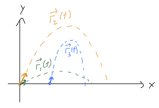
This might sound like a tedious procedure, and it is, but this process (or more sophisticated versions of it) are exactly how numerical solution of differential equations are found. If you use the “NDSolve” function in Mathematica, for instance, it’s doing some version of this iterative procedure to give you the answer. But more importantly, I think this is a more physical way to think about what initial conditions mean, and why we need n of them for an n-th order ODE.
As a side benefit, this construction also establishes uniqueness of solutions: once we fully choose the initial conditions, there is only one possible answer for the solution to the ODE. For Newtonian physics, this means that knowing the initial position and velocity is enough to tell you the unique possible physical path \vec{r}(t) that the system will follow.
Keep in mind that the construction above makes use of initial values, where we specify all of the conditions on our ODE at the same point (same value of t here.) This is a special case of the more general idea of boundary conditions, which can be specified in different ways. (For example, we could find a unique solution for projectile motion by specifying y(0) = y(t_f) = 0 and solving from there to see when our projectile hits the ground again.)
1.4.1 Classifying ODEs and general solutions
Numerical solution is a great tool, but whenever possible we would prefer to be able to solve equations by hand - this is more powerful because we can solve for a bunch of initial conditions at once, and we can have a better understanding of what the solution means.
This brings us to classification of differential equations. There is no algorithm for solving an arbitrary differential equation, even an ODE, and many such equations have no known solutions at all (at which point we go back to numerics.) But there is a long list of special cases in which a solution is known, or a certain simplifying trick will let us find one. Because analytic solution of ODEs is all about knowing the special cases, it’s very important to recognize whether a given equation we find in the wild belongs to one of the classes we have some trick for.
The first such classification we’ll go learn to recognize is the linear ODE (the opposite of which is nonlinear.) To explain this clearly, remember that a linear function is one of the form y(x) = mx + b. To state this in words, the function only modifies x by addition and multiplication with some constants, m and b. A linear differential equation, then, is one in which the unknown function and its derivatives are only multiplied by constants and added together.
For example, if we’re solving for y(x), the most general linear differential equation looks like a_0(x) y + a_1(x) \frac{dy}{dx} + a_2(x) \frac{d^2y}{dx^2} + ... + b(x) = 0. This is a little more complicated since we have two variables now, but if you think of freezing the value of x, then all of the a’s and b are constant and it’s clearly a linear function.
Linearity turns out to be a very useful condition. This isn’t a math class so I won’t go over the proof, but there is a very important result for linear ODEs:
A linear ODE of order n has a unique general solution which depends on n independent unknown constants.
The term “general solution” means that there is a function we can write down which solves the ODE, no matter what the initial conditions are. This function has to contain n constants that can be adjusted to match initial conditions (as we discussed above), but otherwise it is the same function everywhere.
To avoid a common misconception, it’s just as important to be aware of the opposite of the above statement: if we have non-linear ODE, in many cases there is no general solution. There is still always a unique solution if we fully specify the initial values. But for a non-linear ODE the functional form of the solution can be different depending on what the initial values are! See Boas 8.2 for an example.
Alright, so it’s great that we know a general solution is out there, but how do we find it in practice? The answer depends a bit on what kind of equation we have.
The following example is a bonus because you have likely seen this equation before! But if you haven’t, or if you’re not too comfortable with the idea of a “general solution” yet, then you should go through this.
Let’s solve the following ODE: \frac{d^2y}{dx^2} = +k^2 y There is a general procedure for solving second-order linear ODEs like this, but I’ll defer that until later. To show off the power of general solutions, I’m going to use a much cruder approach: guessing. (If you want to sound more intellectual when you’re guessing, the term used by physicists for an educated guess is “ansatz”.)
Notice that the equation tells us that when we take the derivative of y(x) twice, we end up with a constant times y(x) again. This should immediately make you think about exponential functions, since d(e^x)/dx = e^x. To get the constant k out from the derivatives, it should appear inside the exponential. So we can guess y_1(x) = e^{+kx} and easily verify that this indeed satisfies the differential equation. However, we don’t have any arbitrary constants yet, so we can’t properly match on to initial conditions. We can notice next that because y(x) appears on both sides of the ODE, we can multiply our guess by a constant and it will still work. So our refined guess is y_1(x) = Ae^{+kx}. This is progress, but we have only one unknown constant and we need two. Going back to the equation, we can notice that because the derivative occurs twice, a negative value of k would also satisfy the equation. So we can come up with a second guess: y_2(x) = Be^{-kx}. This is very similar to our first guess above, but it is in fact an independent solution, independent meaning that we can’t just change the values of our arbitrary constants to get this form from the other solution. (We’re not allowed to change k, because it’s not arbitrary, it’s in the ODE that we’re solving!)
Finally, we notice that the combination y_1(x) + y_2(x) of these two solutions is also a solution if we plug it back in. So we have y(x) = Ae^{+kx} + Be^{-kx} This is a general solution: it’s a solution and it has two distinct unknown constants, A and B. Thanks to the math result above, if we have a general solution to a linear ODE, we know that it is the general solution thanks to uniqueness.
The whole procedure we just followed might seem sort of arbitrary, and indeed it was, since it was based on guessing! For different classes of ODEs, there will be a variety of different solution methods that we can use. The power of the general solution for linear ODEs is that no matter how we get there, once we find a solution with the required number of arbitrary constants, we know that we’re done. Often it’s easiest to find individual functions that solve the equation, and then put them together as we did here. (Remember, solving ODEs is all about recognizing special cases and equations you’ve seen before!)
Now let’s start to look at some specific methods for solving differential equations. We’re going to begin with first-order ODEs only, because that will open up a new class of physics problems for us to solve: projectile motion with air resistance. Later in the semester, we’ll come back to second-order ODEs.
1.4.2 Separable first-order ODEs
A unique feature of first-order ODEs is that we can sometimes solve them just by doing integrals. A first-order ODE is separable if we can write it in the form F(y) dy = G(x) dx where F(y) and G(x) are just any arbitrary function. Once we’ve reached this form, we can just integrate both sides and end up with an equation relating y to x, which is our solution. This method works even if the ODE is not linear.
A quick aside: splitting the differentials dy and dx apart like this is something physicists tend to do much more than mathematicians (although Boas does it!) Remember that dx and dy do have meaning on their own, as they’re defined to be infinitesmal intervals when we define the derivative dy/dx. That being said, if you’re unsettled by the split derivative above, you can instead think of a separable ODE as one written in the form F(y) \frac{dy}{dx} = G(x) Then we can integrate both sides over dx, \int F(y) \frac{dy}{dx} dx = \int G(x) dx The integral on the left becomes \int F(y) dy by a u-substitution. After we do the integrals, we just have a regular equation to solve for y. The simplest case is when F(y) = 1, i.e. if we have \frac{dy}{dx} = G(x) \\ \int dy = \int G(x) dx \\ y = \int G(x) dx + C (notice that we get one overall constant of integration from the indefinite integrals, just as needed to match the single initial condition for a first-order ODE.)
Solve the following ODE: x \frac{dy}{dx} - y = xy
Solution:
This might not be obviously separable, but let’s do some algebra to find out. We’ll put the y’s together first: x \frac{dy}{dx} = y(1+x) Then divide by x and by y: \frac{1}{y} \frac{dy}{dx} = \frac{1+x}{x} Nice and separated! Next, we split the derivative apart and integrate on both sides: \int \frac{dy}{y} = \int dx\ \frac{1+x}{x} The left-hand side integral will give us the log of y. On the right, it’s easiest to just divide out and write it as 1/x + 1, which gives us two simple integrals: \ln y + C' = \int dx\ \left(1 + \frac{1}{x} \right) = x + \ln x + C'' Just to be explicit, I kept both unknown constants here since we did two indefinite integrals. But since C' and C'' are both arbitrary, and we’re adding them together, we can just combine them into a single constant C = C'' - C'.
Now we need to solve for y. Start by exponentiating both sides: y(x) = \exp \left( x + \ln x + C'' \right) \\ = e^x e^{\ln x} e^{C''} \\ = B x e^x defining one more arbitrary constant. (Since we haven’t determined what the constant is yet by applying boundary conditions, it’s not so important to keep track of how we’re redefining it.)
Finally, we can impose a boundary condition to find a particular solution. Let’s say that y(2) = 2. We plug in to get an equation for B: y(2) = 2 = 2B e^2 \\ \Rightarrow B = \frac{1}{e^2} = e^{-2} and so y(x) = xe^{x-2}.
1.4.3 Linear first-order ODEs
(Note: this solution is discussed in Boas 8.3, but I’m borrowing a little bit of terminology from later sections of chapter 8 to put it in context.)
It turns out that there is a nice and general way to find solutions linear first-order ODEs. The combination of linear and first-order is very restrictive: any such ODE must take the form \frac{dy}{dx} + P(x) y = Q(x).
This is a good place to introduce another technical term, which is homogeneous. A homogeneous ODE is one in which every single term depends on the unknown function y or its derivatives. The equation above does not satisfy this condition, because the Q(x) term on the right doesn’t have any y-dependence; thus, we say this equation is inhomogeneous (some books will use “nonhomogeneous” instead.)
Now, there is another equation which closely related to the one above: \frac{dy_c}{dx} + P(x) y_c = 0. The “c” here stands for complementary; this equation is called the complementary equation to the original. Setting Q(x) to zero gives us an equation that is homogeneous.
Better yet, this equation is separable too: we can readily find that \frac{dy_c}{y_c} = -P(x) dx or doing the integrals, y_c(x) = A e^{-\int dx P(x)}. Of course, this is only a solution if Q(x) happens to be zero. But it turns out to be part of the solution for any Q(x). Suppose that we are able to find some other function y_p(x), which is a particular solution that satisfies the original, inhomogenous equation. Then y(x) = y_c(x) + y_p(x) is also a solution of the full equation. This is easy to see by plugging in: \frac{dy}{dx} + P(x) y = \frac{d}{dx} \left( y_c(x) + y_p(x) \right) + P(x) (y_c(x) + y_p(x)) \\ = \left[\frac{dy_c}{dx} + P(x) y_c(x) \right] + \left[ \frac{dy_p}{dx} + P(x) y_p(x) \right] \\ = 0 + Q(x). This might not seem very useful, because we still have to find y_p(x) somehow. But notice that y_c(x) always has the arbitrary constant A in it. That means that y(x) = y_c(x) + y_p(x) is the general solution to our original ODE (the unique one, because it’s linear, remember!)
This isn’t a mechanics example, but it happens to be one of the simpler cases of a first-order and inhomogeneous ODE problem, so let’s do it anyway. We have an electric circuit consisting of a battery supplying voltage V_0, a resistor with resistance R, and a capacitor with capacitance C:
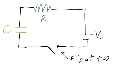
If the capacitor begins with no charge at t=0, we want to describe the current I(t) flowing in the circuit as a function of time. Now, current is the flow of charge, so the charge Q on the capacitor will satisfy the equation I = \frac{dQ}{dt}. The other relevant circuit equations we need are V = IR for the resistor, and Q = CV for the capacitor. Putting these together, we find that the equation describing the circuit is R \frac{dQ}{dt} + \frac{Q}{C} = V_0. The complementary equation is R\frac{dQ_c}{dt} + \frac{Q_c}{C} = 0 which is nice and separable: \frac{dQ_c}{Q_c} = -\frac{1}{RC} dt Integrating gives \ln Q_c = -\frac{t}{RC} + K \Rightarrow Q_c(t) = K' e^{-t/(RC)} Now we need to find the particular solution Q_p. Fortunately, because the right-hand side is just a constant, it’s easy to see that a constant value for Q_p will give us what we want. Specifically, if Q_p = CV_0 then the equation is satisfied, since the derivative term just vanishes.
Finally, we put things together and apply our boundary condition, Q(0) = 0: Q_c(0) + Q_p(0) = 0 = K' e^{-0/(RC)} + CV_0 = K' + CV_0 finding that K' = -CV_0, and thus the finished result is Q(t) = CV_0 \left(1 - e^{-t/(RC)} \right).
So far, everything I’ve said is actually fairly general: this same approach with complementary and particular solutions will be something we use a lot when we get to second-order ODEs.
For any first-order linear ODE, there is actually a trick which will always give you the particular solution for any functions P(x) and Q(x). However, it’s a little complicated to write down, and we won’t need it often. So I won’t cover that here, and instead I’ll refer you to Boas 8.3 for the result. This is one of those formulas that you should know exists, but it’s not worth memorizing - if you find you need it, you can go look it up.
Here, you should complete Tutorial 2A on “Ordinary differential equations”. (Tutorials are not included with these lecture notes; if you’re in the class, you will find them on Canvas.)