9 Symmetry, Conservation Laws, and Equilibrium
9.1 Equilibrium and stability
We’ve seen lots of examples now of putting the Lagrangian formalism to work to easily find equations of motion (accelerations), even for complicated physical systems. However, we haven’t gone much further than that for most problems we’ve seen, mainly because the differential equations we’ve been finding are very difficult to solve!
Still, the equation of motion itself contains a lot of information, even without solving it! In particular, it allows us to identify equilibrium points where the system will remain stationary - and the presence of these points will tell us how the system moves near them, as well!
Let’s go through another example to illustrate some of the interesting things we can learn from just knowing the accelerations.
9.2 Example: bead on a spinning hoop
The setup of this example follows closely from Taylor’s treatment, given as Example 7.6. I usually don’t like to follow the book too closely in class, since you can read it on your own, but this example is important enough that it’s worth seeing twice. I’ll go into a little bit more detail for the setup at the beginning.
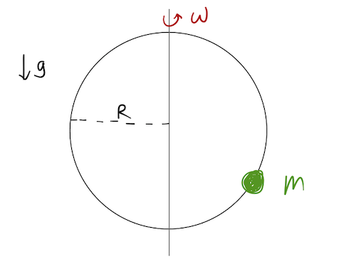
Here’s the basic setup: a bead of mass m and negligible size is threaded on a (frictionless) wire hoop of radius R, which is spinning at constant angular speed \omega. The only force acting is gravity, pointing down in the vertical direction as usual.
As always, we should start by counting degrees of freedom!
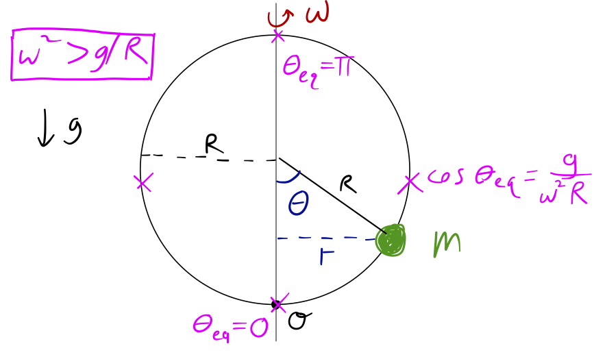
Let’s move on, and (as always) start in an orthogonal coordinate system before changing to our GCs. We’ll define \theta to be the angle of the bead from the center of the hoop, with \theta=0 at the bottom as pictured:
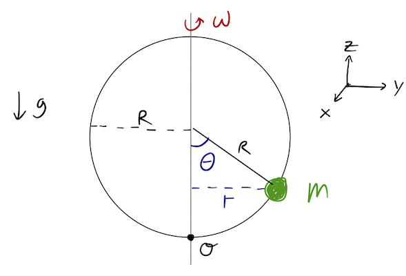
Taking z to be pointing up in the diagram and putting the origin at the bottom of the hoop as pictured, we can write z = R (1 - \cos \theta). Now, we could go on to write out x and y in terms of the angular speed \omega and the distance to the axis, r = R \sin \theta, and then plug in to the kinetic energy in the x-y-z coordinates. However, this will be a mess of trig functions that we’ll have to simplify. There must be a better way!
In fact, any time you see angles as generalized coordinates, you should be thinking about whether you can use one of the other orthogonal coordinate systems you’re familiar with: namely cylindrical (or polar in 2D) and spherical coordinates. As long as you know what the kinetic energy looks like in those coordinates, you can often find the expression you want much more quickly.
Let’s go through the derivation for the kinetic energy in cylindrical coordinates, just to show you how it works (and to help you appreciate the work it will save you.)
To derive this, we’ll start in Cartesian coordinates. The coordinate change is: x = r \cos \phi \\ y = r \sin \phi \\ z = z On notation: you’ll often see \rho for the radius and \theta for the angle here; you can use either one, as long as it’s clear from context what you’re doing. Taking the time derivatives: \dot{x} = \dot{r} \cos \phi - r\dot{\phi} \sin \phi \\ \dot{y} = \dot{r} \sin \phi + r\dot{\phi} \cos \phi \\ \dot{z} = \dot{z} and now, expanding out: T = \frac{1}{2} m (\dot{x}^2 + \dot{y}^2 + \dot{z}^2) \\ = \frac{1}{2} m \left[ \dot{r}^2 \cos^2 \phi + r^2 \dot{\phi}^2 \sin^2 \phi - 2r\dot{r} \cos \phi \sin \phi \right.\\ \left.+ \dot{r}^2 \sin^2 \phi + r^2 \dot{\phi}^2 \cos^2 \phi + 2r\dot{r} \sin \phi \cos \phi + \dot{z}^2 \right] The messy cross-terms all cancel, leaving us with the kinetic energy in cylindrical coordinates: T = \frac{1}{2} m \left[ \dot{r}^2 + r^2 \dot{\phi}^2 + \dot{z}^2. \right]
If you think back to what you’ve learned about circular motion in intro physics, you’ll recognize that the second term is just the tangential component of the velocity vector, v_\phi = r \dot{\phi}.
Now, on to spherical coordinates. The coordinate change is: x = \rho \sin \theta \cos \phi \\ y = \rho \sin \theta \sin \phi \\ z = \rho \cos \theta The following derivation is only in the online notes: I skipped to the result in class, because it’s too much algebra for a lecture. (If you need practice doing algebra/applying the chain rule, try to reproduce the final result without looking at my solution!) \dot{x} = \dot{\rho} \sin \theta \cos \phi + \rho \dot{\theta} \cos \theta \cos \phi - \rho \dot{\phi} \sin \theta \sin \phi \\ \dot{y} = \dot{\rho} \sin \theta \sin \phi + \rho \dot{\theta} \cos \theta \sin \phi + \rho \dot{\phi} \sin \theta \cos \phi \\ \dot{z} = \dot{\rho} \cos \theta - \rho \dot{\theta} \sin \theta This is messy, so let’s do it in pieces organized by where the dot falls. T \supset \dot{\rho}^2 \left(\sin^2 \theta \cos^2 \phi + \sin^2 \theta \sin^2 \phi + \cos^2 \theta \right) = \dot{\rho}^2. Now \dot{\theta}: T \supset \rho^2 \dot{\theta}^2 \left( \cos^2 \theta \cos^2 \phi + \cos^2 \theta \sin^2 \phi + \sin^2 \theta \right) = \rho^2 \dot{\theta}^2. and \dot{\phi}: T \supset \rho^2 \dot{\phi}^2 \left( \sin^2 \theta \sin^2 \phi + \sin^2 \theta \cos^2 \phi \right) = \rho^2 \dot{\phi}^2 \sin^2 \theta. We also have to deal with the various cross terms. First, \dot{\rho} \dot{\theta}: T \supset 2 \dot{\rho} \rho \dot{\theta} \left( \sin \theta \cos \theta \cos^2 \phi + \sin \theta \cos \theta \sin^2 \phi - \sin \theta \cos \theta \right) = 0. Next, \dot{\rho} \dot{\phi}: T \supset 2\dot{\rho} \rho \dot{\phi} \left( -\sin^2 \theta \sin \phi \cos \phi + \sin^2 \theta \sin \phi \cos \phi \right) = 0. and finally, \dot{\theta} \dot{\phi}: T \supset 2 \rho^2 \dot{\theta} \dot{\phi} \left( -\sin \theta \cos \theta \sin \phi \cos \phi + \sin \theta \cos \theta \sin \phi \cos \phi \right) = 0. So finally, we have a reasonably nice-looking result, the kinetic energy in spherical coordinates: T = \frac{1}{2} m \left[ \dot{\rho}^2 + \rho^2 \dot{\theta}^2 + \rho^2 \sin^2 \theta \dot{\phi}^2 \right].
Back to our example: continuing in cylindrical coordinates, we see that r = R \sin \theta \\ "\phi = \omega t" \\ z = R (1 - \cos \theta) (Technical note: \phi = \omega t is actually slightly incorrect, because half of the hoop is at \phi = \pi + \omega t - see the discussion of the clicker question above. Fortunately for us, this ambiguity doesn’t matter, because only \dot{\phi} will end up in our Lagrangian, and \dot{\phi} is the same whether we shift by \pi or not.)
Taking time derivatives, we find \dot{r} = R \dot{\theta} \cos \theta \\ \dot{\phi} = \omega \\ \dot{z} = R \dot{\theta} \sin \theta \\ The kinetic energy is then T = \frac{1}{2} m (\dot{r}^2 + r^2 \dot{\phi}^2 + \dot{z}^2) \\ = \frac{1}{2} m (R^2 \dot{\theta}^2 \cos^2 \theta + (R \sin \theta)^2 \omega^2 + R^2 \dot{\theta}^2 \sin^2 \theta) \\ = \frac{1}{2} mR^2 (\dot{\theta}^2 + \omega^2 \sin^2 \theta). The potential is easy, since we’ve already written out the coordinate change: U = mgz = mgR(1- \cos \theta) and then \mathcal{L} = T - U. Since we have only one coordinate, we’ll only have one Euler-Lagrange equation. Taking derivatives: \frac{\partial \mathcal{L}}{\partial \theta} = mR^2 \omega^2 \sin \theta \cos \theta - mgR \sin \theta \\ \frac{\partial \mathcal{L}}{\partial \dot{\theta}} = mR^2 \dot{\theta} The Euler-Lagrange equation is then \frac{\partial \mathcal{L}}{\partial \theta} = \frac{d}{dt} \left( \frac{\partial \mathcal{L}}{\partial \dot{\theta}} \right) \\ \ddot{\theta} = (\omega^2 \cos \theta - \frac{g}{R}) \sin \theta, where I’ve divided through by mR^2.
Once again, we’re left somewhat unsatisfyingly with an equation of motion which looks very difficult to solve (and there is no analytic solution in terms of ordinary functions, in fact.) However, it turns out there is a lot of information encoded in just this equation; we have everything we need to explore equilibrium points, and how the system behaves near to equilibrium.
9.3 Equilibrium points
An equilibrium point is any configuration of a physical system where the time evolution stops: a system in equilibrium stays in equilibrium, unless it is disturbed by some external influence. Since we only have one coordinate here, this is easy to state mathematically: equilibrium values of \theta occur whenever \ddot{\theta} = 0, or (\omega^2 \cos \theta_{\rm eq} - g/R) \sin \theta_{\rm eq} = 0.
This gives points of equilibrium at \theta_{\rm eq} = 0, \pi, and \cos \theta_{\rm eq} = g / (\omega^2 R) — where the latter two points only exist if \omega is large enough.
Let’s explore the equilibrium points separately, starting with the fixed points at \theta_{\rm eq} = 0 and \pi. I’ll also take the condition \omega^2 < g/R for the moment, so these are the only equilibrium points.
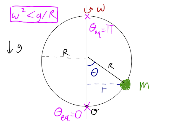
These are the “obvious” equilibrium points, at the very top and bottom of the hoop. At these points, the rotation doesn’t affect the bead at all, and the force of gravity has no component along the wire, so the bead doesn’t move.
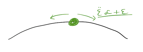
Of course, things that don’t move are boring, so let’s ask a more interesting question: what happens if we nudge our particle slightly away from equilibrium? To be concrete, let’s consider the top point and let \theta = \pi + \epsilon, where \epsilon is a small number. We can Taylor expand about the equilibrium, keeping only first-order terms: \ddot{\epsilon} = (\omega^2 \cos (\pi + \epsilon) - \frac{g}{R}) \sin (\pi + \epsilon) Let’s recall that to Taylor expand a function around an arbitrary point, to first order we write f(x_0 + \epsilon) \approx f(x_0) + \epsilon f'(x_0) + ... so \cos (\pi + \epsilon) \approx \cos \pi - \epsilon \sin \pi = -1 \\ \sin (\pi + \epsilon) \approx \sin \pi + \epsilon \cos \pi = -\epsilon or going back, \ddot{\epsilon} \approx (\omega^2 + \frac{g}{R}) \epsilon. The term in parentheses is always positive, so we find that if we choose any positive \epsilon, the bead will accelerate in the same direction, and the same for negative \epsilon. Thus, \theta_{\rm eq} = \pi is an unstable equilibrium point. If we bump the bead slightly away from equilibrium, it will accelerate away.
On the other hand, if we do the same exercise at the bottom of the hoop, we find that about \theta_{\rm eq} = 0, we have \ddot{\epsilon} \approx (\omega^2 - \frac{g}{R}) \epsilon. Given that \omega^2 < g/R, the term in parentheses is always negative; whatever \epsilon we put in, the acceleration will push it in the opposite direction, back towards \epsilon = 0. This is a stable equilibrium point; if the bead is put in motion near such a point, it will stay near that point.
Notice, by the way, that this first-order equation about the stable equilibrium point is exactly the simple harmonic oscillator equation: \ddot{\epsilon} \approx (\omega^2 - \frac{g}{R}) \epsilon = - \Omega^2 \epsilon. So for small displacements from \theta=0, we see that the bead will oscillate back and forth with frequency \Omega = \sqrt{g/R - \omega^2}. An enormous number of physical systems actually behave like harmonic oscillators near their equilibrium points; this is a fairly deep point which we’ll return to later in the semester.
Now, if we let \omega increase, we notice that eventually (when \omega^2 > g/R), the equilibrium at \theta_{\rm eq} = 0 becomes unstable as well! In terms of forces, the centrifugal force due to the rotation (pushing away from \theta=0) starts to overwhelm the gravitational force (pushing towards \theta=0) even at small \epsilon, and the bead flies off.
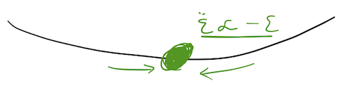
So both equilibrium points are unstable now; does that mean the bead will just spin around in circles from any starting point? Conveniently, we can remember that as soon as this condition is met, two more equilibrium points appear along the sides of the hoop:
Note that since g / (\omega^2 R) is always positive, solutions only exist for \theta_{\rm eq} between 0 and \pi/2; the equilibrium points never reach the top half of the hoop. Going back to the force picture again, these are the points where gravity and centrifugal force are balanced. I leave it as an exercise to show that these two additional equilibrium points are, in fact, both stable (Taylor has the explanation, but try it yourself first!)
(If you’re feeling very ambitious, here’s an amusing question to think about: what happens to the equilibrium points if \omega^2 is exactly equal to g/R?)
That’s all I have to say about equilibrium points for now: hopefully you can appreciate the power of this idea, and the amount of information we can learn about a system even without solving the full differential equation of motion.
9.4 Conserved quantities
By far one of the most important and fundamental theorems in physics is due to Emmy Noether. Noether was a German mathematician and physicist from the early 20th century, a time when women in either field were exceedingly rare, but she persisted in her work despite working in a challenging system, and she made a number of important contributions to mathematics and physics. Noether’s theorem is stated roughly as follows:
“For any continuous symmetry of a physical system, there exists a corresponding conserved quantity.”
You may have heard this statement before, but now that we’re equipped with the Lagrangian, we can actually see Noether’s theorem in action! In fact, we will more or less derive it very simply. (What we’ll really derive is a special case of her theorem for classical systems; the general version of Noether’s theorem applies even to relativistic quantum mechanics, and is immensely powerful.)
When we say that some quantity Q is conserved, in physics we just mean that it is a constant of the motion, or in other words, that dQ/dt = 0. The total energy of a system acted on by conservative forces, E = T + U, is a familiar example of a conserved quantity, but far from the only possibility. In fact, we’ll be able to derive the celebrated principle of conservation of energy from a simpler assumption about symmetry!
How do we see from the Lagrangian what the conserved quantities in a particular physical system are? Suppose we have a Lagrangian in some generalized coordinates, \mathcal{L}(q_i, \dot{q}_i, t). If the Lagrangian is independent of one of the coordinates, then we find: \frac{\partial \mathcal{L}}{\partial q_i} = 0 \Rightarrow \frac{d}{dt} \left( \frac{\partial \mathcal{L}}{\partial \dot{q_i}}\right) = 0. In other words, if the Lagrangian is independent of coordinate q_i, then the quantity \partial \mathcal{L} / \partial \dot{q_i} is conserved! (Some jargon: we say the coordinate q_i which the Lagrangian doesn’t depend on is a cyclic coordinate.)
But what is this derivative, physically? Well, it depends on what the coordinate q_i is. But in any case where we have a continuous symmetry, we can express it in this form, i.e. that the Lagrangian doesn’t depend on the corresponding coordinate. (The rigorous version of Noether’s theorem is a little more complicated and general, but this simple version is enough for the important examples we’re about to see.)
9.4.1 Translation and rotation invariance
Let’s suppose that our Lagrangian describes a single particle, and let q_i be the Cartesian coordinate x. We are only allowing velocity-independent forces, so we know immediately that \frac{\partial \mathcal{L}}{\partial \dot{x}} = \frac{\partial T}{\partial \dot{x}} = m \dot{x} = p_x. Now, if our Lagrangian is also independent of x, then the Euler-Lagrange equation tells us that \frac{\partial \mathcal{L}}{\partial x} = 0 \Rightarrow \frac{dp_x}{dt} = 0. This is the familiar law of conservation of momentum! There is of course nothing special about x, this will work for all three Cartesian coordinates if the Lagrangian is independent of them.
What about the first part of Noether’s theorem; what is the continuous symmetry of our system if \partial \mathcal{L} / \partial x = 0? Well, if the Lagrangian is x-independent, that means we can pick up and move our physical system in x, say x \rightarrow x + \Delta - note that this is a real shift, not just a change of coordinates! - and the equations of motion we find will not change at all. This symmetry is known as translation invariance.
If q_i is some other type of coordinate, we still expect to find a conserved quantity if the Lagrangian is independent of it, but we won’t always find an ordinary linear momentum. Suppose we have a particle moving in two dimensions (x,y), and convert to polar coordinates (r,\theta). As we showed, the kinetic energy looks like T = \frac{1}{2} m (\dot{r}^2 + r^2 \dot{\theta}^2). Now if \partial \mathcal{L} / \partial \theta = 0, the symmetry is called rotational invariance. The basic idea is still that we can shift \theta \rightarrow \theta + \Delta and the physics doesn’t change, but since \theta is an angle it has a different name. The resulting conserved quantity is \frac{\partial \mathcal{L}}{\partial \dot{\theta}} = mr^2 \dot{\theta}, which is exactly the angular momentum of the particle. You might object at this point that angular momentum in general is a vector quantity, \vec{L} = \vec{r} \times \vec{p}. The same was true of the linear momentum above, of course, we were just working with components. What is conserved here is the \hat{\theta} component of \vec{L}, which (since we have just a single particle rotating around the origin) is the only component; \vec{L}_r = \vec{r} \times (p_r \hat{r}) = 0. For more complicated systems the symmetry can be much more complicated to write down, but it has the same consequence; rotational invariance implies conservation of angular momentum.
9.4.2 More general conserved quantities
There are more exotic possibilities if our generalized coordinates are weirder, but usually we work with angles and positions, so these are the conservation laws we usually want to be aware of. For a completely arbitrary coordinate q_i, the conserved quantity if the Lagrangian is invariant under changes in q_i is called the generalized momentum: p_i \equiv \frac{\partial \mathcal{L}}{\partial \dot{q_i}} and \partial \mathcal{L} / \partial q_i = 0 implies \dot{p_i} = 0. By the way, notice that using the generalized momentum, we can rewrite the Euler-Lagrange equation in the form \frac{\partial \mathcal{L}}{\partial q_i} = \dot{p_i}. As you could probably guess, the left-hand side \partial \mathcal{L} / \partial q_i is known as a generalized force, and so the E-L equation looks very similar to Newton’s second law. In fact, if we pick Cartesian coordinates x,y,z, it is exactly Newton’s second law. We won’t use generalized forces again, but we will use generalized momentum for other purposes, so remembering this relationship might help you recall what a generalized momentum looks like.
An important point in all of this is that it’s not always obvious in a given coordinate system whether there is a conserved quantity or not. Consider the following Lagrangian: \mathcal{L} = \frac{1}{2} m (\dot{x}^2 + 2\dot{y}^2) + C(x-y) Now, obviously neither x nor y is a cyclic coordinate. However, we notice that if we apply the shift x \rightarrow x + \epsilon \\ y \rightarrow y + \epsilon then \mathcal{L} doesn’t change at all! In more geometric terms, there is a direction in the xy plane along which our Lagrangian actually is still translation invariant. We can reveal this with a coordinate change, and then identify the conserved momentum: let’s take u = x+y \\ v = x-y and then \dot{u} = \dot{x} + \dot{y} \\ \dot{v} = \dot{x} - \dot{y} Inverting, we find \dot{x} = \frac{1}{2} (\dot{u} + \dot{v}) \\ \dot{y} = \frac{1}{2} (\dot{u} - \dot{v}) so the kinetic energy becomes T = \frac{1}{2} m (\dot{x}^2 + 2\dot{y}^2) \\ = \frac{1}{8} m[(\dot{u}^2 + 2 \dot{u} \dot{v} + \dot{v}^2) + 2 (\dot{u}^2 - 2\dot{u} \dot{v} + \dot{v}^2) ] \\ = \frac{3}{8} m (\dot{u}^2 + \dot{v}^2) - \frac{1}{4} m\dot{u} \dot{v} In these coordinates, the Lagrangian is thus \mathcal{L} = \frac{3}{8} m (\dot{u}^2 + \dot{v}^2) - \frac{1}{4} m \dot{u} \dot{v} + Cv. What do we gain by working so hard to identify a conserved quantity? Well, the big advantage is that it simplifies the time evolution greatly; rewriting our equations of motion using conserved quantities can reduce the number of equations we actually have to solve. You’ll see an important example of this on the homework! As for the current problem, we can take \dot{u} and rewrite it in terms of the conserved quantity p_u: \frac{4p_u}{m} = 3\dot{u} -\dot{v} \Rightarrow \dot{u} = \frac{4p_u}{3m} + \frac{1}{3} \dot{v} Instead of substituting into the Lagrangian, let’s find the v equation of motion first, since we used the u equation of motion to find p_u: \frac{\partial \mathcal{L}}{\partial v} = \frac{d}{dt} \left( \frac{\partial \mathcal{L}}{\partial \dot{v}} \right) \\ C = \frac{d}{dt} \left(\frac{3}{4} m \dot{v} - \frac{1}{4} m \dot{u}\right) \\ = \frac{d}{dt} \left(\frac{3}{4} m \dot{v} - \frac{m}{4} \left[ \frac{4p_u}{3m} + \frac{1}{3} \dot{v} \right]\right) \\ = \frac{d}{dt} \left( \frac{8}{12} m \dot{v} - \frac{p_u}{3} \right) \\ \Rightarrow \ddot{v} = \frac{3C}{2m}. So using our conserved quantity lets us eliminate the u variable completely, and get a single differential equation just involving v! In fact, the result is particularly simple in this case: p_u doesn’t appear in our equations at all once we’ve done the replacement. This makes physical sense, because u and v are orthogonal coordinates, so the motion in the u-direction shouldn’t do anything in the v-direction.
Note that if you just try to set \dot{u} = 0, you will get the wrong answer here! This is because for this system, \dot{u} itself is not a conserved quantity on its own.
9.5 Time translation and energy
There’s one more very important symmetry to consider, and that is time translation. This is one of the most fundamental axioms underpinning not just all of physics, but science as a whole. The idea that repeated identical experiments should have the same outcome is a critical part of the scientific method. We know from Noether’s theorem that with this symmetry must come a conserved quantity, so let’s try to identify it. If we have a physical system which is time-translation invariant, then in terms of the Lagrangian, we must have \frac{\partial \mathcal{L}}{\partial t} = 0. Yes, this is a partial derivative, not a total derivative! We don’t want the entire system to be independent of time - then there’s no motion to consider. We just want to ensure that there is no explicit dependence on time in \mathcal{L}; the most common counterexamples would be some kind of external driving force (time dependence in T) or a time-varying electric or other force field (time dependence in U.)
Above it was obvious that the Euler-Lagrange equations simplified when the derivative with respect to q_i was zero. But remember that there’s also a simplification if we have a functional which doesn’t depend on the independent variable, which is t here. As you showed on the first homework, the condition \partial \mathcal{L} / \partial t = 0 means that we can write the E-L equations in the second form. You only proved it for a single dependent variable, but here’s what it looks like when we have multiple coordinates: \frac{d}{dt} \left(\sum_i \dot{q_i} \frac{\partial \mathcal{L}}{\partial \dot{q_i}} - \mathcal{L} \right) = 0. So the quantity in parentheses is our conserved quantity; it is another new function, and it is called the Hamiltonian. Recognizing the derivative as the generalized momentum, we can rewrite it:
\mathcal{H} = \sum_i p_i \dot{q_i} - \mathcal{L}.
So as long as the Lagrangian does not depend explicitly on time, \partial \mathcal{L} / \partial t = 0, this new quantity is totally conserved: dH/dt = 0. What is the physical meaning of \mathcal{H}? We will explore this question a bit further later in the semester. But notice that if we start in Cartesian coordinates x_i, then the kinetic energy is just T = \frac{1}{2} \sum_i m_i \dot{x_i}^2, which means that p_i = \frac{\partial \mathcal{L}}{\partial \dot{x_i}} = m_i \dot{x_i}, so that \sum_i p_i \dot{q_i} = \sum_i (m_i \dot{x_i} \dot{x_i}) = 2T. Since the Lagrangian is \mathcal{L} = T - U, this means that the Hamiltonian is just \mathcal{H} = \sum_i p_i \dot{q_i} - \mathcal{L} = T + U. So the Hamiltonian in these coordinates is just the total energy! Time translation symmetry leads to conservation of energy as a prediction of Lagrangian mechanics. In fact, \mathcal{H} = T + U will continue to be true in any generalized coordinate system, as long as our change of coordinates doesn’t depend explicitly on time, so \partial q_i / \partial t = 0. (Taylor proves this in the book, have a look at section 7.8.)
The Hamiltonian provides yet another, somewhat new way of thinking about physical systems, now in terms of momenta and positions instead of velocities and positions. In fact, we can use it to write down equations of motion and solve them: as we will prove later on, the Euler-Lagrange equations together with the definition of the generalized momentum leads us to \dot{p_i} = -\frac{\partial H}{\partial q_i} \\ \dot{q_i} = \frac{\partial H}{\partial p_i} These equations (Hamilton’s equations) have twice as many variables, but are only first-order differential equations, which will frequently be an advantage in certain problems. However, since we just learned a new technique in the Lagrangian, we’ll put off Hamiltonian mechanics until we really need it, much later in the semester.