11 Non-Inertial Frames
We’ve spent a lot of time on Lagrangian mechanics, but in this chapter we begin to study mechanics in non-inertial reference frames - frames which are accelerating in one way or another (linear acceleration, or rotation of any kind.)
Of course, Lagrangian mechanics lets us deal with these frames - we’ve done it before - but we still must start in an inertial frame of reference before changing to generalized coordinates within the non-inertial frame. But in many cases, it’s easier and more intuitive to start within an accelerating frame, and the good news is that it’s not so difficult!
Newton’s laws actually can be fixed up to hold in accelerating frames, too; we just have to include some extra “fictitious forces” coming from the acceleration. Despite the name, to an observer in an accelerating frame, the forces are completely real and measurable, as you know if you’ve ever been in a car or an airplane. (In fact, we can in principle make use of the effects we’re about to discuss to decide whether we’re in an accelerating frame experimentally, without any other information.)
11.1 Frames with linear acceleration
Let’s start with a simple physical example to see how acceleration might look in different frames of reference. Suppose we have a cart containing an air cannon, that shoots a ping pong ball straight up into the air:
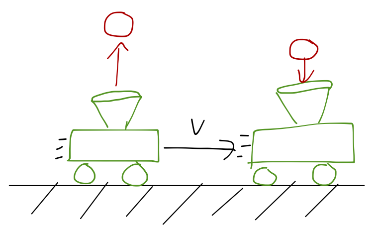
If the cart is at rest, then the ball goes up and comes straight back down, and the cart catches it. Of course, you know that the exact same thing happens if the cart is moving with constant speed, v: the horizontal component of the velocity v_x is identical for the ball and the cart, so it catches the ball again.
In the latter case, to an observer on the cart, the cart is in fact stationary, and it’s obvious that the ball will come back to its starting point. The cart observer’s frame of reference is inertial, since the cart has constant speed, so Newton’s laws are just as valid for them.
Now, what if the cart is accelerating forward with constant acceleration a? Where does the ball land?
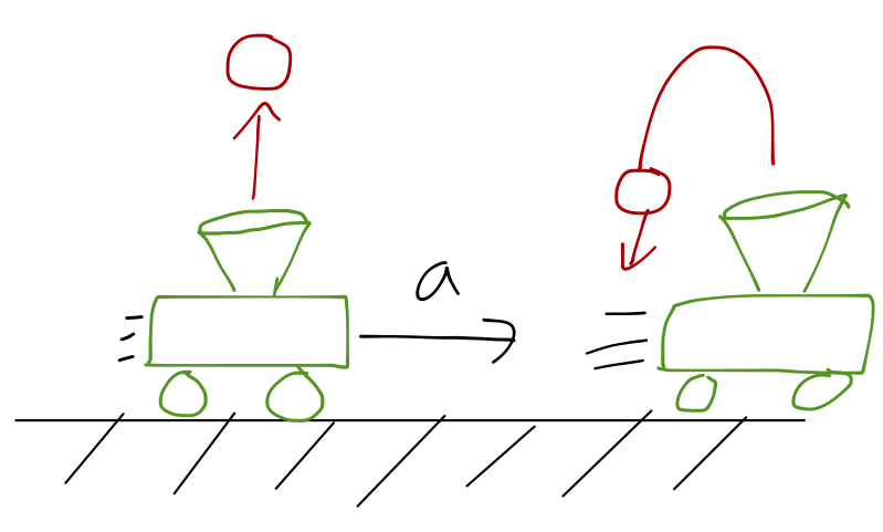
Well, to an outside observer it’s perfectly obvious; the cart accelerates horizontally, the ball does not, so the cart moves out from under the ball and the ball lands behind the cart. But in the frame of reference of an observer on the cart, it looks like the ball is pushed backwards; like there’s some sort of force acting on the ball to accelerate it away from the cart.
Let’s see exactly what’s going on in terms of forces, first in our inertial frame \mathcal{S}_1, and then in the cart frame \mathcal{S}_2. In \mathcal{S}_1, we know that Newton’s laws are valid, i.e. m \ddot{\vec{r_1}} = \vec{F}. where \vec{r_1} is the position of the ball in \mathcal{S}_1. \vec{F} is just the net sum of familiar forces; gravity, the force exerted on the ball by the cart’s air cannon, air resistance, etc. We know how to tally them all and solve for the ball’s acceleration.
Once we’ve solved for the motion of the ball in \mathcal{S}_1, we know how to describe it in \mathcal{S}_2 as well. If the difference in velocity between the two frames is \vec{v}, then the velocity-addition formula applies: \dot{\vec{r_1}} = \dot{\vec{r_2}} + \vec{v}. In words, the velocity of the ball relative to the ground is the velocity relative to the cart, plus the velocity of the cart relative to the ground. Taking the time derivative, we see that \ddot{\vec{r_1}} = \ddot{\vec{r_2}} + \vec{a} We can plug this back into Newton’s law above: m \ddot{\vec{r_2}} = \vec{F} - m \vec{a}. This is almost Newton’s second law, but with an extra term due to the acceleration of \mathcal{S}_2. In fact, to the observer in the cart frame, it looks like Newton’s laws do apply, but there is one extra force compared to what the ground observer sees, namely \vec{F}_{\textrm{inertial}} = -m \vec{a}. This apparent force is opposite the direction of the acceleration. You’ve probably observed this personally: if you’ve ever been on a bus that brakes suddenly, you know that you get pushed forwards by the sudden stop.
Let’s see a practical example of using this fictitious force.
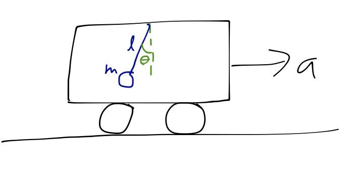
11.1.1 Example: pendulum in an accelerating car
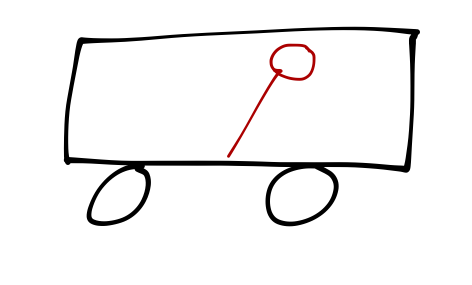
Back to the Newtonian approach! A pendulum of length \ell and mass m is attached to the ceiling of a boxcar, which is accelerating with constant acceleration \vec{a} to the right.
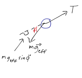
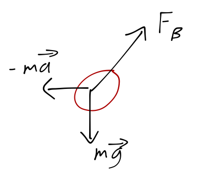
Let’s draw the free-body diagram for the pendulum bob within the accelerating frame. We know that the usual forces of tension and gravity are acting on it, but now we have to include the fictitious inertial force as well:
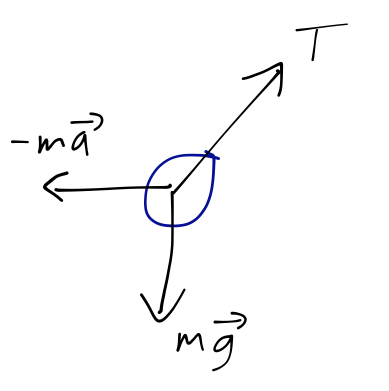
Since gravity and the inertial force are both proportional to mass, we can actually combine them as m\vec{g} - m\vec{a} \equiv m \vec{g_{\textrm{eff}}}, defining the effective gravitational force.
Computing \vec{g_{\textrm{eff}}} \equiv \vec{g} - \vec{a}, which points in the direction \tan^{-1} (a/g), immediately gives us the equilibrium angle. All of this is much simpler than doing everything in full using the Lagrangian - sometimes forces are convenient!
We can even keep going to find the frequency of small oscillations without too much trouble. If we displace a small distance from equilibrium, the restoring force is mg_{\textrm{eff}} \sin (\phi - \phi_{\textrm{eq}}):
which gives the usual equation of motion for a pendulum, m (\ddot{\theta} \ell) = -mg_{\textrm{eff}} \sin (\phi - \phi_{\textrm{eq}}) \\ \ddot{\phi'} = -\frac{g_{\textrm{eff}}}{\ell} \sin \phi' where I’ve replaced \phi' = \phi - \phi_{\textrm{eq}} to make this look exactly like the equation for a simple pendulum. So we can just read off the frequency of small oscillations: \omega = \sqrt{g_{\textrm{eff}}/\ell} = \sqrt{\frac{\sqrt{g^2 + a^2}}{\ell}}.
Here’s a fun variant of this question: suppose instead of a pendulum, we tie a helium balloon to the bottom of the accelerating car.
Which way does it tilt at equilibrium? You might guess to the left, since the inertial force pushes in that direction. But the balloon is also subject to buoyant force - and the inertial force pushes on the air as well as the balloon! This creates a horizontal pressure gradient, so the normally upwards-pointing buoyant force now points to the right:
The buoyant force overcomes both gravity and the external acceleration, and so the balloon tilts to the right, with the motion of the car. (This isn’t completely obvious - to really figure this out we’d need the tools to actually calculate what the buoyant force is.)
There’s a similar effect to watch out for when considering friction in accelerating frames, which you’ll explore on this week’s homework. The thing to remember is that kinetic friction acts to oppose the relative motion of two surfaces, so be careful if one of your surfaces is accelerating!
11.2 Rotating frames
Rotation is another example of acceleration which is a bit more complicated to deal with. If I take the same boxcar and spin it around the center instead:
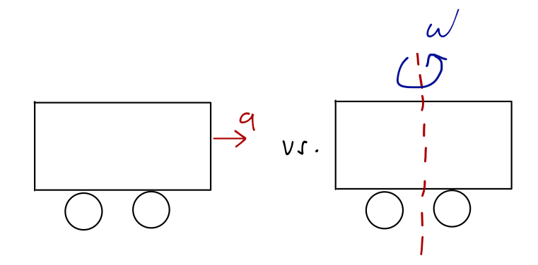
now the system is still accelerating, but the acceleration varies depending on where I stand inside the boxcar.
Rotation is also much more important, because we live on the Earth and the Earth is rotating! It would be very inconvenient to have to do every calculation in our lab frame by first starting in a fixed inertial frame and accounting for the spinning of the Earth. Of course, since you didn’t do this in your freshman labs, you should suspect that the violations of Newton’s laws due to the Earth’s rotation aren’t so big, but it’s certainly important to know exactly what the effects are and what their magnitude is.
Let’s set up some useful formalism, before we go on to derive the fictitious forces. Cross products will appear all over the rotating-frame derivations, so it’s worth keeping the key identities at hand.
For a refresher on the cross product, the right-hand rule, and the determinant formula, see Section 4.2.2. The identities we will use most in this chapter are:
- Antisymmetry: \vec{A} \times \vec{B} = -\vec{B} \times \vec{A}
- Determinant formula: \vec{A} \times \vec{B} = \left|\begin{array}{ccc} \hat{x}&\hat{y}&\hat{z}\\ A_x&A_y&A_z\\ B_x&B_y&B_z\end{array}\right|
- Vector triple product (BAC-CAB): \vec{A} \times (\vec{B} \times \vec{C}) = \vec{B} (\vec{A} \cdot \vec{C}) - \vec{C} (\vec{A} \cdot \vec{B})
- Lagrange’s identity: |\vec{A} \times \vec{B}|^2 = |\vec{A}|^2 |\vec{B}|^2 - (\vec{A} \cdot \vec{B})^2
The cyclic-permutation identity \hat{x}\times\hat{y}=\hat{z} etc. carries over to any orthonormal basis - e.g. in cylindrical coordinates \hat{r}\times\hat{\phi}=\hat{z}.
11.2.1 The angular velocity vector
Back to physics, and to rotation! Recall that rotation involves a rigid body or collection of bodies spinning about an axis. So we need a magnitude (angular velocity, \omega) and a direction (symmetry axis). We can combine these into a vector! If the symmetry axis is \hat{u} (for unit), then \vec{\omega} = \omega \hat{u}. Along a given axis, \vec{\omega} can point up or down. But rotation can also be clockwise or counter-clockwise; so the direction of \vec{\omega} is meaningful. We have to pick a convention! Once again we use the standard right-hand rule convention (the “other right-hand rule”): point your right thumb in the direction of \vec{\omega}, and your fingers curl in the direction of the rotation.
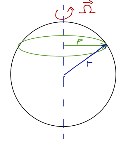
For \vec{\omega} pointing up, the rotation is thus counter-clockwise. For an object rotating around the origin, what is the relation between \vec{\omega} and the ordinary velocity \vec{v}?
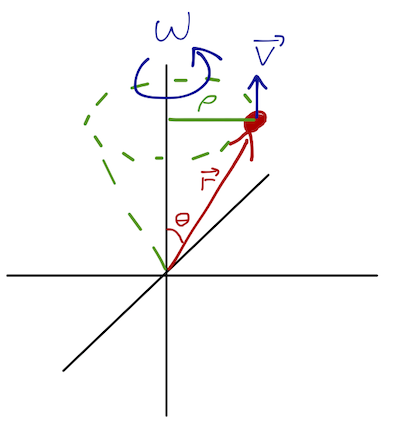
We know the linear speed is v = \rho \omega = (r \sin \theta) \omega, and \hat{v} is directed into the page. This of course looks like a cross product; all we have to do is make sure we get the sign right! Based on the sketch, applying the first “right-hand rule” for vector cross products, we can see that we obtain the correct direction for \vec{v} by choosing \vec{v} = \vec{\omega} \times \vec{r}. ### Time derivatives and rotating frames
Notice that we can rewrite our equation for linear speed as \dot{\vec{r}} = \vec{\omega} \times \vec{r}. In other words, taking the cross product with \omega gives the time derivative of \vec{r}. There’s nothing special about \vec{r} in this equation; it’s actually true for any vector, as we will now see. Let’s use a coordinate system where z points along \vec{\omega}, and x, y are coordinates which are fixed with respect to the rotation.
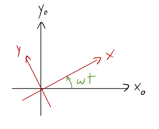
We’ll call the rotating frame \mathcal{S}, with coordinates (x,y,z), and also consider a fixed, inertial frame \mathcal{S}_0, coordinates (x_0, y_0, z_0). At t=0, they are identical, and of course z = z_0 since the rotation is about that axis. Working in the fixed coordinates, we can write one set of unit vectors in terms of the other: \hat{x} = \hat{x_0} \cos \omega t + \hat{y_0} \sin \omega t\\ \hat{y} = \hat{y_0} \cos \omega t - \hat{x_0} \sin \omega t. So if I have a vector which appears to be stationary in my rotating coordinate system, \vec{Q} = Q_x \hat{x} + Q_y \hat{y} + Q_z \hat{z} with all components satisfying dQ_i/dt = 0, then in the fixed coordinates, what I see is \vec{Q} = (Q_x \cos \omega t - Q_y \sin \omega t) \hat{x_0} + (Q_x \sin \omega t + Q_y \cos \omega t) \hat{y_0} + Q_z \hat{z_0}. How does \vec{Q} vary with time in the stationary frame \mathcal{S}_0? Ignoring the fixed \hat{z}_0 component, we find \left(\frac{d\vec{Q}}{dt}\right)_{\mathcal{S_0}} = (-\omega Q_x \sin \omega t - \omega Q_y \cos \omega t) \hat{x_0} + (\omega Q_x \cos \omega t - \omega Q_y \sin \omega t) \hat{y_0} \\ = \omega (\vec{z_0} \times \vec{Q}) \\ = \vec{\omega} \times \vec{Q}, where the subscript reminds us that we’re taking the derivative in the fixed frame \mathcal{S}_0.
What if \vec{Q} depends on time in the rotating frame, i.e. (d\vec{Q}/dt)_{\mathcal{S}} \neq 0? Things don’t change much! In the rotating coordinates, we have (d\vec{Q}/dt)_{\mathcal{S}} = \dot{Q_x} \hat{x} + \dot{Q_y} \hat{y} + \dot{Q_z} \hat{z}. What about the derivative in \mathcal{S}_0? Let’s look at the \hat{x}_0 component and apply the chain rule: (d\vec{Q}/dt)_{\mathcal{S}_0,x} = \frac{d}{dt} \left(Q_x \cos \omega t - Q_y \sin \omega t \right) \hat{x_0} \\ = \left[ (\dot{Q_x} \cos \omega t - \dot{Q_y} \sin \omega t) + (-\omega Q_x \sin \omega t - \omega Q_y \cos \omega t)\right] \hat{x_0}. The first term here is exactly how the (x-component of) (d\vec{Q}/dt)_{\mathcal{S}} looks in the fixed coordinates \mathcal{S}_0! We find a similar result for the other two components, which means that in general,
\left( \frac{d\vec{Q}}{dt}\right)_{\mathcal{S}_0} = \left( \frac{d\vec{Q}}{dt}\right)_{\mathcal{S}} + \vec{\omega} \times \vec{Q}.
You can remember this as something like another velocity-addition rule; the motion of \vec{Q} that we see in the inertial frame (d\vec{Q}/dt)_{\mathcal{S}_0} is equal to its motion relative to the rotating frame (d\vec{Q}/dt)_{\mathcal{S}}, plus the motion of the rotating frame relative to the inertial frame, \vec{\omega} \times \vec{Q}.
Now we’re ready to tackle Newton’s second law, much like we did for linear acceleration.
11.2.2 Newton’s second law in a rotating frame
Here I’ll switch notation as the book does, and use capital \vec{\Omega} to represent the relative angular velocity of \mathcal{S}. This reminds us that \Omega is a special vector related to changing frames; we could still have some angular motion represented by an \omega within the rotating frame.
As before, start with Newton’s 2nd law in the fixed frame: m \left(\frac{d^2 \vec{r}}{dt^2} \right)_{\mathcal{S}_0} = \vec{F}. Now we start rewriting the derivatives, using the relation we just found. \left(\frac{d^2 \vec{r}}{dt^2} \right)_{\mathcal{S}_0} = \left(\frac{d}{dt}\right)_{\mathcal{S}_0} \left(\frac{d\vec{r}}{dt} \right)_{\mathcal{S}_0} \\ = \left(\frac{d}{dt}\right)_{\mathcal{S}_0} \left[ \left( \frac{d\vec{r}}{dt}\right)_{\mathcal{S}} + \vec{\Omega} \times \vec{r} \right] \\ = \left(\frac{d}{dt}\right)_{\mathcal{S}} \left[ \left( \frac{d\vec{r}}{dt}\right)_{\mathcal{S}} + \vec{\Omega} \times \vec{r} \right] + \vec{\Omega} \times \left[ \left( \frac{d\vec{r}}{dt}\right)_{\mathcal{S}} + \vec{\Omega} \times \vec{r} \right]. All the time derivatives are now in frame \mathcal{S} which is our destination, so let’s go back to dot notation. Expanding the first term gives us \left(\frac{d}{dt}\right)_{\mathcal{S}} \left[ \dot{\vec{r}} + \vec{\Omega} \times \vec{r} \right] = \ddot{\vec{r}} + \dot{\vec{\Omega}} \times \vec{r} + \vec{\Omega} \times \dot{\vec{r}} and the second term gives \vec{\Omega} \times \left[ \dot{\vec{r}} + \vec{\Omega} \times \vec{r} \right] = \vec{\Omega} \times \dot{\vec{r}} + \vec{\Omega} \times (\vec{\Omega} \times \vec{r}). Plugging back into Newton’s second law above and moving all of the new terms over to the other side, we reverse some of the cross products (remember: \vec{A} \times \vec{B} = -\vec{B} \times \vec{A}.) So we have finally:
m \ddot{\vec{r}} = \vec{F} + 2m \dot{\vec{r}} \times \vec{\Omega} + m (\vec{\Omega} \times \vec{r}) \times \vec{\Omega} + m \vec{r} \times \dot{\vec{\Omega}} \\ = \vec{F} + \vec{F}_{\textrm{cor}} + \vec{F}_{\textrm{cf}} + \vec{F}_{\textrm{Euler}}.
As promised, this is more complicated than linear acceleration - we have three fictitious forces to worry about:
- Centrifugal force: \vec{F}_{\rm cf} = m (\vec{\Omega} \times \vec{r}) \times \vec{\Omega}
- Coriolis force: \vec{F}_{\rm cor} = 2m \dot{\vec{r}} \times \vec{\Omega}
- Euler force: \vec{F}_{\rm Euler} = m \vec{r} \times \dot{\vec{\Omega}} By the way, we could have just as easily derived all of these fictitious forces by way of the Lagrangian approach instead! We know in frame \mathcal{S}_0, the Lagrangian is given by \mathcal{L} = \frac{1}{2} mv^2 - U(\vec{r}) = \frac{1}{2} m \left|\left( \frac{d\vec{r}}{dt}\right)_{\mathcal{S}_0}\right|^2 - U(\vec{r}) so, substituting the derivative just as we did above, the Lagrangian in frame \mathcal{S} is just \mathcal{L} = \frac{1}{2}m |\dot{\vec{r}} + \vec{\Omega} \times \vec{r}|^2 - U(\vec{r}). The Euler-Lagrange equation for \vec{r} will then give us exactly the same set of fictitious forces (as you will see on the next homework assignment!)
Let’s start to get a feeling for these rotational forces by considering a simple example.
11.2.3 Example: the merry-go-round
Our example is a merry-go-round: a simple, circular platform which is rotating at some angular speed \Omega. Let’s take the rotation to be counter-clockwise, so \vec{\Omega} = \Omega \hat{z}. Because we’re looking at motion on a two-dimensional surface which is perpendicular to the motion, i.e. \vec{r} and \vec{\Omega} are always perpendicular, the dynamics will be simplified somewhat.
Suppose we’re sitting on the merry-go-round at \vec{r} = r\hat{x}, and \vec{\Omega} is in the +\hat{z} direction. Let’s start with the centrifugal force.
We start with the general expression: \vec{F}_{\rm cf} = m (\vec{\Omega} \times \vec{r}) \times \vec{\Omega} To evaluate this, we apply the RHR - carefully! First, the vector \vec{\Omega} \times \vec{r} is tangential to the motion, pointing in the +\hat{y} direction. So (\vec{\Omega} \times \vec{r} ) \times \vec{\Omega} points outwards, the +\hat{x} direction. This is, of course, just opposite the direction of the centripetal acceleration which is applied in a stationary external frame to keep us moving in a circle.
Another way to see the direction is through one of the cross-product identities we wrote out last time: (\vec{\Omega} \times \vec{r}) \times \vec{\Omega} = \vec{r} (\vec{\Omega} \cdot \vec{\Omega}) - \vec{\Omega} (\vec{\Omega} \cdot \vec{r}). Since in this case \vec{\Omega} \cdot \vec{r} = 0, the force is in the \vec{r} direction; moreover, we can see easily that its magnitude is |\vec{F}_{\rm cf}| = m \Omega^2 r.
Actually, we can use this same vector identity to step back and find a more general insight about the centrifugal force. Forget the merry-go-round for a moment, and suppose that \vec{\Omega} and \vec{r} are completely general. As long as we orient our coordinate system so that \vec{\Omega} = \Omega \hat{z}, then \vec{r} (\vec{\Omega} \cdot \vec{\Omega}) - \vec{\Omega} (\vec{\Omega} \cdot \vec{r}) = \Omega^2 (r_x \hat{x} + r_y \hat{y} + r_z \hat{z}) - \Omega^2 r_z \hat{z} \\ = \Omega^2 (r_x \hat{x} + r_y \hat{y}) \\ = \Omega^2 \vec{\rho}, where \vec{\rho} is the radius in cylindrical coordinates. So (again, if \vec{\Omega} = \Omega \hat{z}), \vec{F}_{\textrm{cf}} = m \Omega^2 \rho \hat{\rho}. Centrifugal force is always directed radially outwards from the axis of rotation! This should match your intuition, of course, but it’s good to see it coming out of the math.
Finally, the Euler force will only appear when the ride is starting or stopping, i.e. when some angular acceleration is applied. If you return to your seat at +\hat{x} on the merry-go-round, you will feel the Euler force when the ride ends, and a \dot{\vec{\Omega}} vector appears (in the -\hat{z} direction - can you see why?) The Euler force is then directed in the +\hat{y} direction, pushing you forwards (it’s a backwards force when the ride starts.)
Let’s do a more involved (but still qualitative) example, again in a plane perpendicular to the rotation, to improve our intuition for looking in two different frames.
11.2.4 Example: “orbit” on a turntable
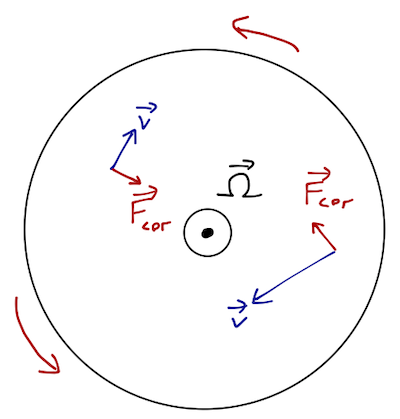
Consider an air-hockey puck, moving on the surface of a frictionless turntable. The turntable is rotating at constant angular speed \omega, but we don’t know the direction (yet.) We are standing on the turntable, and when we release the puck with initial speed v_0, we observe this trajectory:
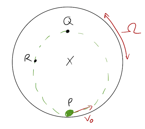
So the puck appears to follow an “orbit”, and comes back to point P. Let’s try to break down the motion. We know that there are only two forces in play here: the centrifugal force and Coriolis force (no Euler force since \vec{\Omega} is constant.) \vec{F}_{\rm cf} = m(\vec{\Omega} \times \vec{r}) \times \vec{\Omega} \\ \vec{F}_{\rm cor} = 2m \dot{\vec{r}} \times \vec{\Omega} Actually, we can simplify the centrifugal force again since \vec{r} is in a plane perpendicular to \vec{\Omega}: \vec{F}_{\rm cf} = m \Omega^2 \vec{r}. How do they combine to give us the trajectory shown? Let’s start at point Q, the turning point of the orbit:
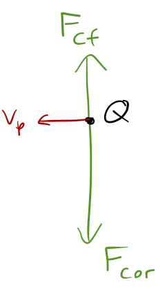
Since Q is above the center, the centrifugal force has to be pointing up, away from the center. But for the puck to turn around as we observe, the net force at Q must be towards the center, which tells us that the Coriolis force is pointing the other way.
Thanks to this information, we now have experimental evidence for which way the turntable is rotating! Since F_{\rm cor} is pointing down at Q, while \vec{v} is to the left, the rotation must be clockwise, i.e. \vec{\Omega} points into the page (-\hat{z} direction.)
Knowing the direction of rotation, we can move on to consider the forces at other points, like R:

Here the centrifugal force points to the left, and the Coriolis force down and to the right. We don’t know the magnitude precisely, but we can see the effect on the speed of the puck; since F_{\rm cor} is perpendicular to the velocity vector it doesn’t cause any change in speed. On the other hand, F_{\rm cf} has a component in the direction of motion, so we see the puck is speeding up in the rotating frame at R. If we look on the other side of the center, we’ll see it’s slowing down.
One more important realization is that although the motion looks rather complicated in the rotating frame, we should remember that it’s always equally valid to step back to the lab frame and look at the problem in a different way. What does our “orbit” look like in the lab frame?
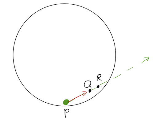
Yes, it’s simply a straight line! It has to be a straight line, because in the inertial lab frame, all the fictitious forces disappear, and there are no other forces in this problem. Points P, Q and R are all simply rotating around, intersecting the straight-line trajectory of the puck at different times.
Note that this was a bit of a tricky question; there’s no actual “orbital” motion here. Although the puck returns to point P, it only does so once, before flying off the table entirely! Returning to point P also, clearly, requires a very specific choice of v_0 relative to \Omega.
This lab-frame picture should emphasize to you that there really isn’t anything mysterious about the fictitious rotational forces, even if they look strange and intimidating. The centrifugal force is very familiar; it exactly corresponds with the centripetal acceleration, which is provided to keep an object moving in a circular path.
The Coriolis effect, as we’ve seen, is nothing more than what happens when something is moving in a straight line from point A to point B, but point B rotates away, causing an apparent deflection. Finally, the Euler force is exactly the acceleration in the tangential direction that occurs when speeding up or slowing down the rotation speed \Omega.
To demystify the Coriolis force a bit, here’s a nice little demo from MIT:
11.3 Earth as a rotating frame
Now that we’ve studied the fictitious forces appearing in rotating frames in more detail, let’s turn to the most interesting application: the effects of the Earth’s rotation.
We should start by setting up our coordinates, of course! The Earth is (roughly) a spherical body, so we’ll use spherical coordinate (r, \theta, \phi); on the surface of the Earth, r = R_E is taken to be constant. The radius of the Earth is roughly R_E \approx 6400\ \textrm{km}. The Earth is spinning about an axis, of course, but which way does the angular velocity vector point?
Once more, we should note the numeric value of the rotation: it’s straightforward to see that \Omega_E = \frac{2\pi}{24\ \rm{h} \times 3600\ \rm{s/h}} = 7.3 \times 10^{-5}\ \rm{rad}/\rm{s}. Be aware that the standard angular coordinates used to locate positions on the Earth are longitude and latitude, and these are not quite the same as ordinary spherical coordinates! Let’s look at a sketch:
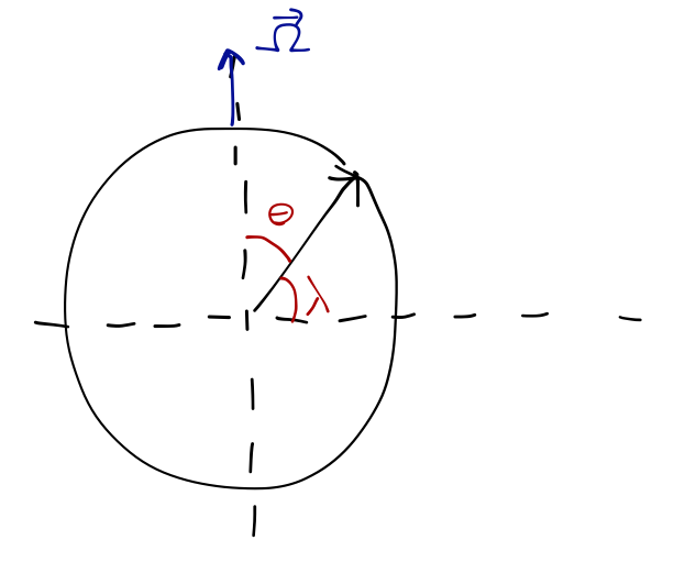
Longitude is exactly the azimuthal spherical angle \phi which you can’t see in this side-on view. The zero of longitude is set at the prime meridian, which is a north-south line passing through Greenwich in the UK. On the other hand, latitude is almost the standard spherical coordinate \theta, but not quite! Latitude \lambda has its zero at the equator, while our usual \theta is zero at the pole (specifically, the north pole.)
More confusingly, \lambda isn’t usually labeled as positive or negative, but “north” or “south”. So to convert from \lambda to \theta, we have two formulas: \theta = \pi/2 - \lambda\ \textrm{(north)} \\ \theta = \pi/2 + \lambda\ \textrm{(south)}. So Boulder is at \lambda = 40^\circ N, which is at \theta = 50^\circ. The more familiar coordinate \theta is also known as the co-latitude.
11.3.1 Centrifugal force on the Earth
Let’s think about the Earth’s centrifugal force first. As we saw before, orienting the Earth’s angular velocity vector in the +\hat{z} direction leads to a centrifugal force that points outwards from the axis. In cylindrical coordinates, we have simply:
\vec{F}_{\textrm{cf}} = m \Omega_E^2\ \rho \hat{\rho}.
We can immediately see that the effect will be zero at the poles (where \rho = 0), and maximum at the equator. (If you step on a scale at the equator, you will actually weigh slightly less than you do at the north or south pole!)
If we want to actually calculate effects at the Earth’s surface, we should switch back to spherical coordinates, since cylindrical coordinates aren’t very convenient. In spherical coordinates, we can easily look up that the unit vector \hat{\rho} becomes \hat{\rho} = \sin \theta \hat{r} + \cos \theta \hat{\theta}. The magnitude of \rho, meanwhile, can be easily determined from our sketch above to be \rho = R_E \sin \theta so combining, the centrifugal force anywhere on the Earth’s surface is: \vec{F}_{\textrm{cf}, E} = m \Omega_E^2 R_E (\sin^2 \theta\ \hat{r} + \sin \theta \cos \theta\ \hat{\theta}). The radial component is proportional to m, and directly opposite the gravitational force! Thus, if we try to measure g at different latitudes, our results will be slightly different due to the centrifugal force (and also due to the fact that the Earth isn’t perfectly spherical.)
What about the magnitude? We see that on the equator (\theta = \pi/2), a_{\textrm{cf}} = \Omega_E^2 R_E \approx 0.034\ \rm{m}/\rm{s}^2 so you can see that this effect is always small compared to the gravitational acceleration of 9.8 {\rm m}/{\rm s}^2. (If you weigh 150 pounds, the difference between your weight at the pole and the equator resulting from this effect is about 0.5 pounds.)
Away from the poles and equator, we also have a tangential centrifugal force. This is proportional to mass again, so it looks like a modification of F_g, but now the direction changes too! Explicitly, we can write \vec{g} = \vec{g}_0 + \vec{F}_{\textrm{cf},E}/m = (-g_0 + \Omega_E^2 R_E \sin^2 \theta) \hat{r} + \Omega_E^2 R_E \sin \theta \cos \theta\ \hat{\theta}. This causes a deflection angle \alpha between the direction of gravity \vec{g}_0 and the direction of free-fall acceleration \vec{g}. The deflection is maximized at \theta = \pm45^\circ, where \tan \alpha \approx \alpha = \frac{\Omega_E^2 R_E/2}{g} = \frac{0.017\ \rm{m/s}^2}{9.8\ \rm{m/s}^2} \approx 0.0017\ \rm{rad} \approx 0.1^\circ. In principle, this is a measurable deflection! In practice, defining “vertical” is extremely difficult; almost any experiment you can think of will give you the direction of \vec{g} and not \vec{g}_0. So we generally define “vertical” to include the centrifugal terms, and deal with the difference in the few, very specialized cases where it matters.
Should we worry that now that we’ve changed the definition of vertical, the \hat{\theta} component will change our conclusion about how our perceived weight varies over the surface of the Earth? Weight is just given by mg, which we can now work out explicitly: |\vec{g}| = (g_0 - \Omega_E^2 R_E \sin^2 \theta)^2 + \Omega_E^4 R_E^2 \sin^2 \theta \cos^2 \theta \\ = g_0^2 + \Omega_E^4 R_E^2 \sin^4 \theta - 2g_0 \Omega_E^2 R_E \sin^2 \theta + \Omega_E^4 R_E^2 \sin^2 \theta \cos^2 \theta \\ = g_0^2 - \Omega_E^2 R_E \sin^2 \theta (2g_0 - \Omega_E^2 R_E). We find another correction term which is always negative and proportional to \sin^2 \theta, but since \Omega_E^2 R_E \ll g_0, this extra effect is even smaller by another factor of 1/300 or so.
11.3.2 The Coriolis force on the Earth
The Coriolis force acts on moving objects according to their velocity \vec{v} = \dot{\vec{r}} with respect to the rotating frame. \vec{F}_{\textrm{cor}} = 2m \dot{\vec{r}} \times \vec{\Omega} = 2m \vec{v} \times \vec{\Omega}. The direction of the force depends on the direction of \vec{v}. One helpful observation: if you replace 2m with q and \vec{\Omega} with \vec{B}, this is just the expression for magnetic force, which might help your intuition for how the Coriolis force acts.
On the Earth, the Coriolis force tends to be dwarfed by even the centrifugal force. For an object moving at, say, 40 m/s (an MLB fastball) and perpendicular to \Omega, the acceleration is a_{\textrm{cor},E} = 2v \Omega_E = 2(40\ \rm{m/s}) (7.3\times 10^{-5}\ \rm{s}^{-1}) \approx 0.006\ \rm{m/s}^2. But the Coriolis effect can become important either for objects moving much faster, or for objects in motion for a long time so that the cumulative effect matters.
What is the direction of the Coriolis force? For motion parallel to the Earth’s surface, we can use a top-down picture from above the north pole:
For any direction of \vec{v}, the deflection due to the Coriolis force is to the right on this diagram (which shows the entire northern hemisphere.) If you’re not convinced, use the right-hand rule: rotate your hand around to keep \vec{\Omega} fixed and move \vec{v}.
In the southern hemisphere, the effect reverses; we can draw the same diagram looking down from the south pole, but now \Omega is into the page. So the Coriolis force deflects motion to the left in the southern hemisphere.
Going beyond just the direction, you can see that the magnitude of the Coriolis effect varies over the surface of the Earth, depending whether the motion is tangential or radial (i.e. throwing an object or dropping it.) For tangential motion, the effect is largest at the poles and zero at the equator for the north/south direction (as we saw), and is constant for east/west motion. For radial motion, the Coriolis force is largest at the equator and zero at the poles.
How about some examples? I mentioned that the Coriolis effect is important for fast motion, or long-lasting motion. The most famous example of fast motion is artillery, specifically naval guns - many battleships would fire shells with muzzle velocities of around 800 m/s, for example. Naval engagements at long range require accurate calculations for the shells to end up where you aim, and the Coriolis force is one of the effects taken into account!
(True story: when British warships were sent to the Falkland Islands in 1982, they noticed that their guns were missing their targets by a substantial amount! Eventually it was noticed that the firing solutions were correcting for the Coriolis effect by including the latitude, but not whether it was north or south latitude, so the force had the wrong sign - the shells were missing by exactly twice the Coriolis deflection.)
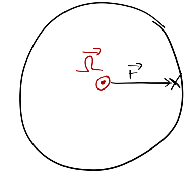
Another major application of the Coriolis effect is the explanation of hurricanes and typhoons. These are powerful, rotating storm systems (“tropical cyclones”); they don’t form within 500 miles or so of the equator, and they rotate in opposite directions in the two hemispheres. Hurricanes in the northern hemisphere rotate counterclockwise. You might have guessed clockwise, because the Coriolis force is to the right, but we have to be careful!
A hurricane has a defining central eye, which is a low-pressure region: air rushes in towards the eye. As the air rushes in, the Coriolis force deflects it to the right:
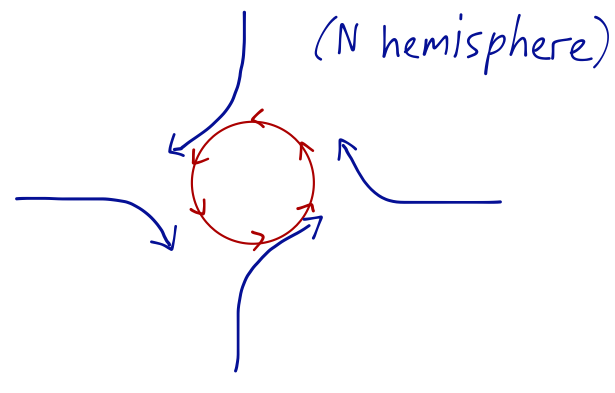
So although an individual air molecule moves clockwise, the net flow of air around the low-pressure region is counter-clockwise, matching the observations. This also explains why cyclones don’t form near the equator; the reversal of direction as we cross the equator doesn’t support a vortex, instead the net flow of air goes westwards (this gives the “trade winds”.)
We can also answer the question, why does a hurricane have an “eye”, a calm, cloudless, low-pressure region in the center? Since a hurricane is rotating, it will carry its own set of internal fictitious forces. In particular, the centrifugal force will push air molecules outwards from the center, offsetting the pressure gradient that’s pulling them inwards if the air molecules are moving fast enough (and they speed up towards the center, conserving angular momentum: the fastest wind speeds are in the “eye wall” just outside the eye.)
The same argument, in principle, could be applied to water rushing down a sink drain. Here’s some experimental homework for you: have a close look at your sink or shower drain next time you use it. Does the water drain clockwise, or counter-clockwise?
Odds are you couldn’t tell; if it happened to be counter-clockwise, then it wasn’t caused by the Coriolis force! It’s an urban myth that the Coriolis force causes all water to drain counter-clockwise in the northern hemisphere - the force is too small, and effects like initial angular momentum overwhelm it in your sink. Some toilets will consistently drain in one direction, but that’s because of design - the water is jetted in one direction.
In principle, if your water had no initial angular momentum and you watched very carefully, you would see a net counter-clockwise rotation. Physicists have confirmed this experimentally, but it is extremely difficult!
11.3.3 Example: Coriolis force and free-fall
Now let’s do a more quantiative treatment of how the Coriolis force can deflect free-fall motion. Following Taylor, it’s helpful to start by setting up a local Cartesian coordinate system, and writing this equation out in components. Here it is:
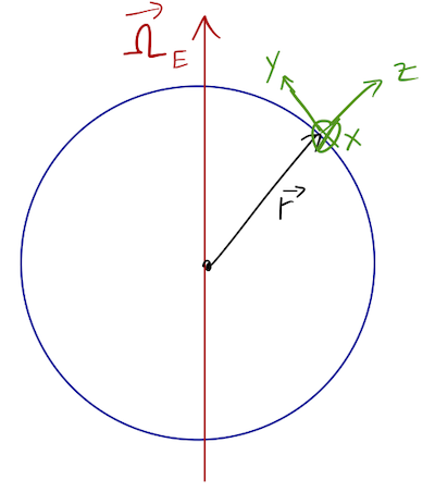
We can think of our three coordinates (x,y,z) as “east”, “north”, and “up” respectively, which are all correct identifications as long as we don’t move too far away. In our local coordinates, we see that the rotation vector \vec{\Omega}_E has components along \hat{y} and \hat{z}: \vec{\Omega}_E = (0, \Omega_E \sin \theta, \Omega_E \cos \theta) so in these coordinates, we see that \dot{\vec{r}} \times \vec{\Omega}_E = \left| \begin{array}{ccc} \hat{x} & \hat{y} & \hat{z} \\ \dot{x} & \dot{y} & \dot{z} \\ 0 & \Omega_E \sin \theta & \Omega_E \cos \theta \end{array} \right| \\ = \Omega_E (\dot{y} \cos \theta - \dot{z} \sin \theta, -\dot{x} \cos \theta, \dot{x} \sin \theta). Including the gravitational (plus centrifugal) acceleration, our three equations of motion are thus \ddot{x} = 2\Omega_E (\dot{y} \cos \theta - \dot{z} \sin \theta) \\ \ddot{y} = -2\Omega_E \dot{x} \cos \theta \\ \ddot{z} = -g + 2\Omega_E \dot{x} \sin \theta. These equations do have an analytic solution, but it’s somewhat complicated; remembering that \Omega_E is very small, we can instead carry out a perturbative solution, solving the equations repeatedly with successively more powers of \Omega_E included.
11.4 Perturbation theory
To deal with these equations, we’re going to use a technique known as perturbation theory.
Let me start by setting up the formal idea of a perturbative solution; this is an extremely common technique for solving physics problems, which you’ve certainly already seen used in a couple of particular cases (but probably not the general technique.)
Here is the setup: suppose that we have found an equation of motion of the form \ddot{r} = F(r, \epsilon) where \epsilon is a small, dimensionless parameter, and F is some totally arbitrary function. Of course, the obvious thing to do is expand the right-hand side in \epsilon: \ddot{r} = F(r, 0) + \epsilon \frac{\partial F}{\partial \epsilon} + ... and then try to solve that equation. However, it’s a common situation that this equation is still not easy to solve, and we can only really get the \epsilon = 0 version of the motion. Also, there are situations in which \epsilon is small but not too small, and we care about the discarded \epsilon^2 piece.
This brings us back to the idea of perturbation theory, which is to pre-emptively expand our solution in \epsilon as well, like this: r(t) = r^{(0)}(t) + \epsilon r^{(1)}(t) + \epsilon^2 r^{(2)}(t) + ... The piece of the solution r^{(n)} which is proportional to \epsilon^n is called the n-th order solution. (Note that I don’t have the 1/2 in front of the \epsilon^2 term that would be there for a Taylor expansion. It would have been fine to include it, as long as we remember it when we put the pieces back together to get r(t)!)
Now we have a nice, systematic way to approach our solution. We start by simply solving the equation with \epsilon set to zero: \ddot{r}{}^{(0)} = F(r^{(0)}, 0) giving us the “zeroth-order” solution for r(t). Now we keep the first term in \epsilon on both sides: \ddot{r}{}^{(0)} + \epsilon \ddot{r}{}^{(1)} = F(r^{(0)}, 0) + \epsilon \frac{\partial F}{\partial \epsilon}(r^{(0)}, 0) Now, the beauty of this equation is that since \epsilon is just a parameter, it must be true for any value of \epsilon, which means the \epsilon^1 pieces on both sides have to be equal: \epsilon \ddot{r}^{(1)} = \epsilon \frac{\partial F}{\partial \epsilon}(r^{(0)}). This is a much simpler differential equation for \ddot{r}^{(1)}, especially because we already know what r^{(0)}(t) is on the right-hand side. Plus, it’s very straightforward to keep going and find r^{(2)}(t) by keeping the \epsilon^2 pieces.
The key to using a perturbative solution is that you need a dimensionless small parameter to do the expansion in - never try to expand in something dimensionful in a physics problem, you’ll probably just confuse yourself! The formal expressions will start to look a bit complicated if we keep going, so let’s go back to our freefall problem.
Here are our equations of motion again: \ddot{x} = 2\Omega_E (\dot{y} \cos \theta - \dot{z} \sin \theta) \\ \ddot{y} = -2\Omega_E \dot{x} \cos \theta \\ \ddot{z} = -g + 2\Omega_E \dot{x} \sin \theta. We suspect that perturbation theory can be used here, because we know the effects of the Earth’s rotation \Omega_E are often very small. But what is our small parameter? It’s not simply \Omega_E, because that would be dimensionful. Instead, I’ll take the expansion parameter to be \epsilon = \Omega_E T, where T is the total time our object spends in free-fall. This makes physical sense: the longer our object is falling, the more important the fictitious forces will be, no matter how small \Omega_E is! (You might worry about the fact that we don’t exactly know T yet, but it will end up cancelling out anyway in favor of the actual time t. If you don’t like T being the total time, just take it to be a fixed reference time that is definitely large compared to the freefall time, but not so large that \epsilon isn’t tiny.)
We start at zeroth-order in \Omega_E T, which basically just means we set \Omega_E = 0. Here we know the answer already: the only acceleration is \ddot{z} = -g, and we find the usual free-fall motion. Setting initial conditions as starting from rest with x=y=0 and z=h, we have x = x^{(0)}(t) = 0 \\ y = y^{(0)}(t) = 0 \\ z = z^{(0)}(t) = h - \frac{1}{2} gt^2, where the superscript (0) reminds us that these are zeroth-order; they don’t depend on \Omega_E at all.
Now, on to first order. Notice what happens if we plug our series expansion into the x equation of motion above: \ddot{x} = 2\frac{\epsilon}{T} (\dot{y} \cos \theta - \dot{z} \sin \theta) \\ \ddot{x}^{(0)} + \epsilon \ddot{x}^{(1)} + ... = 2\frac{\epsilon}{T} \left[ (\dot{y}^{(0)} + \epsilon \dot{y}^{(1)} + ...) \cos \theta - (\dot{z}^{(0)} + \epsilon \dot{z}^{(1)} + ...) \sin \theta \right] Since we already know the zeroth-order solution, we just want to determine what \ddot{x}^{(1)} is here, which means we want all of the terms with one power of \epsilon on the right-hand side. Since there’s already an \epsilon outside the brackets, and since y^{(0)}(t) = 0, we see there’s only one: \epsilon \ddot{x}^{(1)} = -2\frac{\epsilon}{T} \dot{z}^{(0)} \sin \theta = 2\frac{\epsilon}{T} gt \sin \theta. This is the only equation in which \dot{z} appears, so we see that the other equations are unchanged to this order: formally, \ddot{y}^{(0)} + \epsilon \ddot{y}^{(1)} + ... = 0 + \mathcal{O}(\epsilon^2) \\ \ddot{z}^{(0)} + \epsilon \ddot{z}^{(1)} + ... = -g + \mathcal{O}(\epsilon^2) or reducing to equations just for the first-order pieces, \ddot{x}^{(1)} = 2g\frac{t}{T} \sin \theta \\ \ddot{y}^{(1)} = 0 \\ \ddot{z}^{(1)} = 0. Note that the 1/T in the equation for the x-acceleration fixes up the dimensions…
You can see what’s happening here: at zeroth order, our object only moves in the z-direction, which means that the speed in the x and y directions is small. Motion in the z-direction gives a Coriolis deflection purely in the x-direction.
To get the complete solution, we have to put all the pieces back together: for example, we have \ddot{x}(t) \approx \ddot{x}^{(0)}(t) + \epsilon \ddot{x}^{(1)}(t) = 2\Omega_E g t \sin \theta Now we just integrate twice and impose the initial conditions to find our complete first-order solution: x(t) \approx \frac{1}{3} \Omega_E gt^3 \sin \theta, \\ y(t) \approx 0, \\ z(t) \approx h - \frac{1}{2} gt^2. Taylor stops at this point, but I say why not keep going to second order?
Applying this procedure to the other two equations, you should be able to arrive at the result \ddot{x}^{(2)} = \frac{2}{T} (\dot{y}^{(1)} \cos \theta - \dot{z}^{(1)} \sin \theta) \\ \ddot{y}^{(2)} = -\frac{2}{T} \dot{x}^{(1)} \cos \theta \\ \ddot{z}^{(2)} = \frac{2}{T} \dot{x}^{(1)} \sin \theta. This is easier to solve than it looks, since we know that both \dot{y}^{(1)} and \dot{z}^{(1)} are zero; plugging in \dot{x}^{(1)} = (gt^2/T) \sin \theta and integrating the other two equations gives us {y}^{(2)} = -\frac{1}{6} \frac{gt^4}{T^2} \cos \theta \sin \theta \\ {z}^{(2)} = \frac{1}{6} \frac{gt^4}{T^2} \sin^2 \theta so for the full second-order solution, we add each of these terms multiplied by \epsilon^2 = (\Omega_E T)^2: x(t) = \frac{1}{3} \Omega_E gt^3 \sin \theta + \mathcal{O}(\epsilon^3) \\ y(t) = -\frac{1}{6} \Omega_E^2 gt^4 \cos \theta \sin \theta + \mathcal{O}(\epsilon^3) \\ z(t) = h - \frac{1}{2} gt^2 + \frac{1}{6} \Omega_E^2 gt^4 \sin^2 \theta + \mathcal{O}(\epsilon^3) Hopefully you can appreciate that this is a really nice trick for solving differential equations when a small parameter is involved! Everything we’ve done is totally rigorous; you will find the same answer if you solve the system exactly (Mathematica can do this, e.g.) and then series expand the solutions that you find.
You should be careful with boundary conditions when applying this technique, since the total solution has to satisfy those, not just the individual pieces. (Typically, as happened here, the zeroth-order solutions will handle any nontrivial boundary conditions, and then the higher-order terms all simply vanish at the boundaries.)
We should emphasize that, justifying our series expansion treatment, this is a small (but not completely negligible) effect. The book gives the example of a 100m mine shaft at the equator, which gives a horizontal deflection at first order in \Omega_E of about 2 cm. The (zeroth-order) time in freefall is \sqrt{2h/g} = 4.5 seconds, so \epsilon = \Omega_E T \approx 3 \times 10^{-4} - small indeed, so we trust our expansion! Indeed, if we look at 45 degrees latitude instead, then the (first-order) x-deflection is 1.6 cm, but the predicted (second-order) y-deflection is only 1.8 micrometers.
One last nice example of motion on the rotating Earth is the Foucault pendulum; I won’t cover this in lecture, but Taylor does it in detail in chapter 9.9. If you haven’t seen one in person before, check out the operating Foucault pendulum in the base of the Gamow tower right here in our own physics building (you can see it from the outside.)