14 Coupled oscillators and nonlinear dynamics
Before diving in, a quick reminder of the single mass on a spring (covered fully in Chapter 6). For a spring with constant k and equilibrium position x_0, the restoring force and potential are F_k = -k(x-x_0), \qquad U_k = \tfrac{1}{2} k (x-x_0)^2, and the Lagrangian \mathcal{L} = \tfrac{1}{2} m\dot{x}^2 - \tfrac{1}{2} k(x-x_0)^2 gives the equation of motion \ddot{x} = -\frac{k}{m}(x-x_0), with general solution x(t) = A \cos(\omega t - \delta), \qquad \omega = \sqrt{k/m}. A and \delta are fixed by the initial conditions. We’ll start with the undamped, undriven case throughout this chapter.
14.1 Coupled oscillators
We turn now to systems of coupled oscillators; in terms of classical mechanics, when you see the word “oscillator” you should think “mass on a spring”. The simplest example of a coupled oscillator is then a system of masses, which are connected by springs.
This seems like much more of a special case than rigid body rotation, and it is; any everyday object in this room is a rigid body, but a coupled oscillator isn’t nearly as common, and probably makes you picture some contraption with air carts and springs which was dreamed up by a physics professor to confuse you in lab. But the motion of coupled oscillators is much more important once we start to look at the world on an atomic scale.
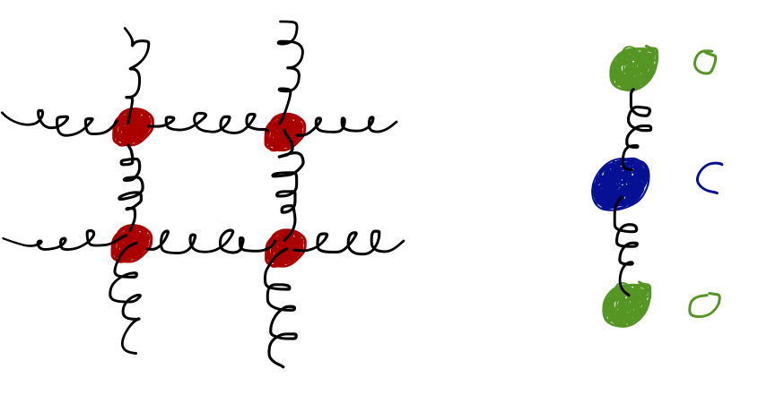
In fact, I misled you just now because the room is full of coupled oscillators, in the air, within the objects around us. Molecular bonds behave an awful lot like springs when we consider small displacements, which are the only kind important for determining, say, the vibrational energy states of a CO_2 molecule, or of a crystalline solid:
Physical applications aside, our study of coupled oscillators will also be an introduction to some important mathematical ideas, involving the solution of systems of differential equations, which will apply beyond the cases where we can describe everything in terms of springs and Hooke’s law.
Now let’s move on to our first example of a coupled oscillator: two masses, connected by three springs.
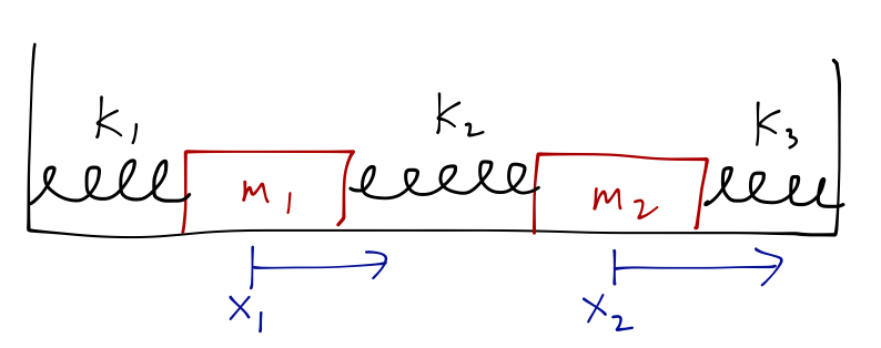
To make things easier, let’s start by defining generalized coordinates x_1 and x_2 as pictured, so that equilibrium is at x_1 = x_2 = 0. We could still solve this in terms of forces, but let’s use the Lagrangian again. We will have two kinetic terms (two masses), T = \frac{1}{2} m_1 \dot{x_1}^2 + \frac{1}{2} m_2 \dot{x_2}^2 The potential energy has three terms, one for each spring: from the diagram, we see that U = \frac{1}{2} k_1 x_1^2 + \frac{1}{2} k_2 (x_1 - x_2)^2 + \frac{1}{2} k_3 x_2^2 Putting it together, our Lagrangian takes the form \mathcal{L} = \frac{1}{2} m_1 \dot{x_1}^2 + \frac{1}{2} m_2 \dot{x_2}^2 - \frac{1}{2} k_1 x_1^2 - \frac{1}{2} k_2 (x_1 - x_2)^2 - \frac{1}{2} k_3 x_2^2 \\ = \frac{1}{2} m_1 \dot{x_1}^2 + \frac{1}{2} m_2 \dot{x_2}^2 - \frac{1}{2} (k_1 + k_2) x_1^2 - \frac{1}{2} (k_2 + k_3) x_2^2 + k_2 x_1 x_2. Writing the Euler-Lagrange equations as usual gives us m_1 \ddot{x_1} = -(k_1 + k_2) x_1 + k_2 x_2 \\ m_2 \ddot{x_2} = k_2 x_1 - (k_2 + k_3) x_2. If we take away the middle spring (k_2 = 0), then the oscillators decouple, and this reduces to a pair of simple harmonic oscillators as you should expect. But otherwise, this is a pair of coupled differential equations. Since the derivative of x_1 depends on x_2 and vice-versa, we can’t just solve one equation and plug in to the other; we have to solve both at once.
One approach would be to just assume that the solution is still given by sines and cosines, and just plug in to see what we get. If you try that, you will end up with a mess! For the simple harmonic oscillator, we can cancel the cosine out after plugging in to the equation, just giving us the simple relation \omega^2 = k/m. But here, we have two cosines with (possibly) two different frequencies; we can’t simplify easily!
Before we go on to the general solution, notice that there’s one other special case we’ve seen before; if we set k_1 = k_3 = 0, then only the middle spring remains, and we have \ddot{x_1} = \frac{k_2}{m_1} (x_2 - x_1) \\ \ddot{x_2} = \frac{k_2}{m_2} (x_1 - x_2) You solved this on one of the homework sets; we can decouple the equations by switching coordinates to the center-of-mass position X = \frac{1}{m_1 + m_2} (m_1 x_1 + m_2 x_2) and the relative displacement d = x_1 - x_2. The CM equations end up being trivial (no external forces), and for the displacement we found \ddot{d} = \ddot{x_1} - \ddot{x_2} = -\frac{k_2}{m_1} d - \frac{k_2}{m_2} d = -\frac{k_2}{\mu} d where \mu is the usual reduced mass, \mu = m_1 m_2 / (m_1 + m_2).
Note that this particular change of coordinates won’t help us with all three springs present! You can try, but you won’t find the same simplification, basically because the equation for the CM’s motion is not trivial; the springs attached to the walls provide “external forces”. But that doesn’t mean that there isn’t some clever choice of coordinates which will let us decompose this into two separate equations. (As you probably expect, finding these coordinates will involve an eigenvalue equation.)
Let’s go back to the equations of motion with all three springs present: m_1 \ddot{x_1} = -(k_1 + k_2) x_1 + k_2 x_2 \\ m_2 \ddot{x_2} = k_2 x_1 - (k_2 + k_3) x_2. We can write this more compactly as a matrix equation, starting by gathering the two coordinates into a vector: \vec{x} \equiv \left( \begin{array}{c} x_1 \\ x_2 \end{array} \right). In this notation, both the left- and right-hand sides of the equation of motion can be written as matrix-vector products. By inspection, \left( \begin{array}{cc} m_1 & 0 \\ 0 & m_2 \end{array} \right) \left( \begin{array}{c} \ddot{x_1} \\ \ddot{x_2} \end{array} \right) = -\left( \begin{array}{cc} k_1 + k_2 & -k_2 \\ -k_2 & k_2 + k_3 \end{array} \right) \left( \begin{array}{c} x_1 \\ x_2 \end{array} \right). or more compactly,
\overset{\leftrightarrow}{M} \ddot{\vec{x}} = -\overset{\leftrightarrow}{K} \vec{x}, where \overset{\leftrightarrow}{M} is the mass matrix and \overset{\leftrightarrow}{K} is the matrix of spring constants. This is the matrix form of the simple harmonic oscillator equation.
Notice that both matrices involved are symmetric; for the mass matrix, this is automatic because it is diagonal. For the matrix of spring constants, the symmetry arises from the fact that the middle spring is only sensitive to changes in its length, not which side is being pushed or pulled. (In terms of forces, the symmetry is sort of a manifestation of Newton’s third law.)
14.2 Normal modes and normal frequencies
The simple structure of the matrix equation above motivates us to look for solutions in terms of sines and cosines. In particular, let’s try a solution where the entire vector \vec{x} oscillates at a single frequency: \vec{x} = \left( \begin{array}{c} A_1 \\ A_2 \end{array} \right) \cos \omega t This might seem like a big oversimplification to you, but suppose we find any such solutions \vec{x}_1(t) and \vec{x}_2(t) that work. We can then see that if we take \vec{x}_3 = a_1 \vec{x}_1 + a_2 \vec{x}_2, then \mathbf{M} \ddot{\vec{x}}_3 = \mathbf{M} (a_1 \ddot{\vec{x}}_1 + a_2 \ddot{\vec{x}}_2) \\ = a_1 (-\mathbf{K} \vec{x}_1) + a_2 (-\mathbf{K} \vec{x}_2) \\ = -\mathbf{K} (a_1 \vec{x}_1 + a_2 \vec{x}_2) \\ = -\mathbf{K} \vec{x}_3. In other words, this differential equation obeys the superposition principle; linear combinations of solutions give us another solution. I’ll invoke a fundamental result at this point from the mathematics of differential equations, and state that we only need two such solutions here to have the completely general solution.
The two is not because our matrices are two by two here. It’s because the differential equation is second order. However, this is allowing the vector in front of the cosine to have N independent components. If we fix the vector in front, as we’re about to, then we need 2N such solutions.
With a solution of this form, we have \ddot{\vec{x}} = -\omega^2 \vec{x}, which immediately lets us rewrite the vector equation above as \overset{\leftrightarrow}{M} (-\omega^2 \vec{x}) = - \overset{\leftrightarrow}{K} \vec{x} \\ (\overset{\leftrightarrow}{K} - \omega^2 \overset{\leftrightarrow}{M}) \vec{x} = 0. This is a big, important equation! Let’s notice a few things about it:
- There is, as usual, a trivial solution to this equation: \vec{x} = 0. I’ve emphasized that trivial solutions are usually boring from the point of view of a physicist, and here that’s obviously true; the trivial solution corresponds to no motion at all.
- If the masses are equal, then \overset{\leftrightarrow}{M} = m \overset{\leftrightarrow}{1}. In that case, this is the eigenvector equation for the matrix \overset{\leftrightarrow}{K}, and we identify the eigenvalues as \lambda = \omega^2 m.
- If the masses aren’t equal, this is called a generalized eigenvalue equation. The solutions are not really eigenvectors of \overset{\leftrightarrow}{K}, nor are they eigenvectors of the combined matrix \overset{\leftrightarrow}{K} - \omega^2 \overset{\leftrightarrow}{M} (they are actually vectors which live in the null space of the combined matrix, to use the proper terminology.)
Much like the ordinary eigenvalue equation, the condition for non-trivial solutions to exist is that the determinant of the combined matrix must vanish: \det(\overset{\leftrightarrow}{K} - \omega^2 \overset{\leftrightarrow}{M}) = 0. As in the case of rigid bodies, the fact that the matrices involved here are symmetric (and thus so is their combination) guarantees that we can always find n solutions for an n \times n matrix, that is, n independent vectors \vec{x} which satisfy the generalized eigenvalue equation. (The symmetry of the inertia tensor guaranteed that any rigid body always has three principal axes, you’ll recall.)
The solutions \vec{x}_i to the generalized eigenvalue equation are called normal modes, and the corresponding eigenvalues \omega_i are the normal frequencies. In general there will not be two normal frequencies, but N for N objects (which makes the mass and spring constant matrices N \times N). For each normal mode we can write two solutions to the differential equation — sine and cosine — which gives us the required 2N solutions to construct the general solution.
Like the inertia tensor, there is of course no guarantee that the normal frequencies are unique, or even non-zero; we only know that we can always write down N independent normal modes. Unlike the inertia tensor, we don’t have to make the normal modes orthogonal, just linearly independent, although orthogonal will sometimes be more convenient.
The best way to understand this is just to see it, so here’s a nice PhET simulation:
14.3 Functions of matrices
There’s a much more direct way to arrive at the normal-mode solution, which should help clarify why the normal-mode approach works in the first place. But to understand the direct approach, we need to take a detour into some math, to define how to take functions of matrices.
We’ve seen before how to define basic operations on matrices, including powers; the matrix A^n is just obtained by multiplying A together, n times. We can make use of this to define matrix functions in terms of their power series. For example, the exponential of a matrix is defined to be: \exp(A) = \sum_{n=0}^{\infty} \frac{1}{n!} A^n. In principle, this series always converges, so we can always define the exponential of a matrix in this way. In practice, it’s an infinite series, so we can only find an explicit answer when there is some repeating pattern in the powers of A (or if A^m = 0 for some m, which terminates the series.) For example, let’s try A = \left(\begin{array}{cc} 1&2 \\ 0&1 \end{array}\right). The first few powers are easy to compute: A^2 = \left(\begin{array}{cc} 1&4 \\ 0&1 \end{array} \right) \\ A^3 = \left(\begin{array}{cc} 1&6 \\ 0&1 \end{array} \right) \\ (...)\\ A^n = \left(\begin{array}{cc} 1&2n \\ 0&1 \end{array} \right) So we can rewrite the infinite sum as \exp(\mathbf{A}) = \sum_{n=0}^\infty \frac{1}{n!} \left( \begin{array}{cc} 1& 2n \\ 0 & 1 \end{array} \right). We can evaluate the sum inside each entry of the matrix separately: \sum_{n=0}^\infty \frac{1}{n!} = e, \\ \sum_{n=0}^\infty \frac{2n}{n!} = 2\sum_{n=0}^\infty \frac{1}{(n-1)!} = 2\sum_{m=0}^\infty \frac{1}{m!} = 2e, giving the result \exp(\mathbf{A}) = \left( \begin{array}{cc} e & 2e \\ 0 & e \end{array} \right)
\exp(\mathbf{A}) is not the same as taking the exponential of the individual elements of the matrix! Element-wise exponentiation would have given us e^2 in the upper-right corner and 1 in the other corners, both of which are wrong.
Of course, not every matrix is guaranteed to have a nice, recurring expression for A^n that we can sum up like this. But there’s one other class of matrices that’s particularly easy to exponentiate, which are the diagonal matrices. Since for an m \times m diagonal matrix, \mathbf{A} = \left(\begin{array}{cccc} a_1 &&&\\ &a_2&& \\ &&...& \\ &&&a_m \end{array} \right) \Rightarrow \mathbf{A}^n = \left(\begin{array}{cccc} a_1^n &&&\\ &a_2^n&& \\ &&...& \\ &&&a_m^n \end{array} \right) we can do the sum no matter what the components are: \exp(\mathbf{A}) = \left(\begin{array}{cccc} e^{a_1} &&&\\ &e^{a_2}&& \\ &&...& \\ &&&e^{a_n} \end{array} \right) Other functions can also be defined as power series, but we have to be careful about the existence of the result in general. Square root is a much trickier function. Certainly, we can define B to be the matrix square-root of A as long as it satisfies the equation B^2 = A. But writing this as a function isn’t particularly nice; for one thing, there is often not a unique solution to this equation; many matrices can be square roots for a given A. (The humble 2x2 identity matrix has an infinite number of square roots! Most 2x2 matrices have four.) Neither is existence of a solution guaranteed; there are some matrices with no square root.
The first piece of good news is that if A is diagonal, then its square root is both unique and easy to find: \sqrt{ \mathbf{A}} = \left(\begin{array}{cccc} \sqrt{a_1} &&&\\ &\sqrt{a_2}&& \\ &&...& \\ &&&\sqrt{a_n} \end{array} \right) (Notice that this matrix isn’t quite unique; we could have put minus signs into any of the diagonal entries, and it would still square to A. But like the square-root symbol, we take the positive root by convention. The square root matrix with all positive eigenvalues is sometimes called the principal square root.)
Of course, most matrices aren’t diagonal. But as long as the matrix is diagonalizable, i.e. as long as there exists a coordinate change which we can apply to make it diagonal, then we can always find the square root (or other functions) in this way. You’ll recall this was true for the inertia tensor, working in the principal axes - coordinates given by the eigenvectors. The same will be true for the coupled oscillator problem, because the matrices \mathbf{M} and \mathbf{K} are both real and symmetric.
14.4 General solution for the coupled oscillator
What if we just try to solve the matrix equation M \ddot{\vec{x}} = -K \vec{x} like the ordinary simple harmonic oscillator? First, we “divide out” the mass, by multiplying on the left by M^{-1}: \ddot{\vec{x}} = -(M^{-1} K) \vec{x} Now, as a reminder, one way to write the solution to the scalar SHO is by using a complex exponential: x(t) = A e^{i\omega t} \Rightarrow \ddot{x} = -\omega^2 A e^{i\omega t} = -\omega^2 x. The complex number is a convenience, of course; the position of a cart x(t) is still a real number. By taking the real part, or careful choices of the (possibly complex) coefficient A, we can make sure we get a real x(t) in the end. I’m just using the complex notation because it’ll make the following explanation easier, but we could just write sine/cosine too.
So, why don’t we just do the same thing for our matrix equation? If \vec{x}(t) = e^{\pm i \sqrt{M^{-1} K} t} \vec{A} then \ddot{\vec{x}}(t) = - (M^{-1} K) \vec{x} and we can immediately see that the most general possible solution to the equation is just given by adding these two solutions up: \vec{x}(t) = e^{i\sqrt{M^{-1} K} t} \vec{x}_+ + e^{-i\sqrt{M^{-1} K} t} \vec{x}_- where \vec{x}_+, \vec{x}_- are determined by the 2N initial conditions as usual (starting position and speed of each mass, say.)
To take these functions of our matrix M^{-1} K, we have to diagonalize it, which means we just need to find its eigenvalues and eigenvectors: (M^{-1} K - \lambda_i \mathbf{1}) \vec{v}_i = 0 and the eigenvalue equation is \det(M^{-1} K - \lambda \mathbf{1}) = \det(M) \det(K - \lambda M) = 0. This gives us back what I called the “generalized eigenvalue equation” last time; now you can really see that this is just the normal eigenvalue equation, but for the more complicated matrix M^{-1} K! (We know \det{M} \neq 0, so don’t worry about that term.) Because the combined matrix M^{-1} K is still real and symmetric, like the inertia tensor we are guaranteed to be able to diagonalize in any problem.
In a coordinate system defined by the eigenvectors of this matrix, we know that e.g. in the 2x2 case M^{-1} K \rightarrow \left( \begin{array}{cc} \lambda_1 & 0 \\ 0 & \lambda_2 \end{array} \right) = \left( \begin{array}{cc} \omega_1^2 & 0 \\ 0 & \omega_2^2 \end{array} \right), and our solution becomes simply \vec{x}(t) = \left( \begin{array}{cc} e^{i\omega_1 t} & 0 \\ 0 & e^{i\omega_2 t} \end{array} \right) \vec{x}_+ + \left( \begin{array}{cc} e^{-i\omega_1 t} & 0 \\ 0 & e^{-i\omega_2 t} \end{array} \right) \vec{x}_-, where \vec{x}_+ and \vec{x}_- are constants determined by the initial conditions of our problem. It’s vital to remember that we’ve changed coordinates here, to what are known as the normal coordinates, \xi_i. As usual, we can expand any vector in components of either coordinate system: \vec{x} = x \hat{x} + y \hat{y} = \xi_1 \hat{\xi}_1 + \xi_2 \hat{\xi}_2.
- Find the equations of motion, i.e. solve for the accelerations \ddot{\vec{x}}. Make sure to expand around equilibrium, so \ddot{\vec{x}} = 0 if \vec{x}=0.
- Write the equations in the form \mathbf{M} \ddot{\vec{x}} = -\mathbf{K} \vec{x}.
- Solve the generalized eigenvalue equation \det(\mathbf{K} - \omega^2 \mathbf{M}) = 0 for the normal frequencies, \omega_i.
- Solve the generalized eigenvector equation (\mathbf{K} - \omega_i^2 \mathbf{M})\vec{\xi}_i = 0 for the normal modes, \vec{\xi}_i.
- The general solution is then \vec{x}(t) = \sum_i \vec{\xi}_i A_i \cos (\omega_i t - \delta_i), where initial conditions will determine A_i and \delta_i.
As we’ve just investigated, all of this is equivalent to simply stating that the general solution is \vec{x}(t) = \exp \left(\pm i \sqrt{\mathbf{M}^{-1} \mathbf{K}} t \right) \vec{A} and then diagonalizing the matrix \mathbf{M}^{-1} \mathbf{K} in order to evaluate the exponential and square-root functions. Once again, diagonalization is at the center of what we’re doing here, just as it was for the inertia tensor, which is why we rely on the same eigenvalue/eigenvector procedure to find our “clever choice of coordinates”. There’s sort of a mental map you can remember between inertia tensors and coupled oscillators, in fact:
- Normal coordinates \leftrightarrow body-frame coordinates
- Normal frequencies \leftrightarrow principal moments
- Normal modes \leftrightarrow principal axes
14.5 Expansion at equilibrium
Our study of coupled oscillators is much more general than it might seem. In fact, a huge number of physical processes can be reduced to a coupled harmonic oscillator description. Michael Peskin (a famous particle physicist) goes so far as to define physics as “that subset of human experience that can be reduced to coupled harmonic oscillators”.
The ubiquitous nature of the coupled SHO isn’t mysterious; it comes from the fact that we are often interested in small changes of a system around some equilibrium. Suppose we have just written down the Lagrangian and wrote out the equations of motion for some physical process. If we gather all of the accelerations on one side, we can almost always write the equations of motion in the form \ddot{q_i} = f_i(q_1, q_2, ..., q_n) for a system with n degrees of freedom. Now assume that we’ve located an equilibrium point, \{Q_i\}, for which the system will remain at rest, i.e. f_i(Q_1, Q_2, ..., Q_n) = 0. We can consider small perturbations of the system around the (constant) equilibrium point: q_i(t) = Q_i + \eta_i(t) where the \eta_i are all small numbers. Without knowing anything at all about the functions f_i, we can deal with these small perturbations by Taylor expanding: f(q_1, q_2, ..., q_n) = f(Q_1, Q_2, ..., Q_n) + \sum_{j=1}^{n} \left.\frac{\partial f_i}{\partial q_j}\right|_{q=Q} (q_j - Q_j) + ... \\ = \sum_{j=1}^n \left.\frac{\partial f_i}{\partial q_j}\right|_{q=Q} \eta_j + ... Since (in our expansion) \ddot{q_i} = \ddot{\eta_i}, after the Taylor expansion our equations of motion become \ddot{\eta}_i = \sum_{j=1}^n \left.\frac{\partial f_i}{\partial q_j}\right|_{q=Q} \eta_j This can be re-written as a matrix equation, \ddot{\vec{\eta}} = \overset{\leftrightarrow}{F} \vec{\eta}. So any physical system close enough to equilibrium will behave as a simple harmonic oscillator! This is exactly the equation we’ve been studying for the masses and springs; for that particular system we identify \overset{\leftrightarrow}{F} = -\overset{\leftrightarrow}{M}^{-1} \overset{\leftrightarrow}{K}. As always, the general solution is \eta_i(t) = \sum_i \vec{v}_i \left[ A_i e^{\sqrt{\lambda_i} t} + B_i e^{-\sqrt{\lambda_i} t} \right], where \lambda_i and \vec{v}_i are the eigenvalues and eigenvectors of \overset{\leftrightarrow}{F}.
In the case of the masses and springs, the eigenvalues of F were all negative (because M^{-1} K has all positive eigenvalues), so the only solution was simple harmonic motion - sines and cosines with angular frequency \sqrt{\lambda}. More generally, not every equilibrium point is totally stable; sometimes the equilibrium is unstable, and the time-dependence is exponential instead of oscillating.
Of course, a concern with a completely general \mathbf{F} is that it will not necessarily be real and symmetric - something we relied upon to ensure that we can find a full set of eigenvectors and eigenvalues in order to write this solution down. In the most general case, this is not guaranteed. However, we can easily see that for any system described by a Lagrangian, \mathbf{F} is indeed real and symmetric. We can write the most general possible Lagrangian in the form \mathcal{L} = \frac{1}{2} \sum_{i,j} T_{ij}(q_1, q_2, ..., q_n) \dot{q}_i \dot{q}_j - V(q_1, q_2, ..., q_n), where T_{ij} is a symmetric tensor that can also depend on coordinates. (A simple example we’ve seen before is given by the kinetic terms in spherical coordinates.) Now, the Euler-Lagrange equations take the form \frac{d}{dt} \left( \frac{\partial \mathcal{L}}{\partial \dot{q_i}} \right) = \frac{\partial \mathcal{L}}{\partial q_i} This will be messy if we write it out in general, but if we appeal to our equilibrium expansion q_i(t) = Q_i + \eta_i(t) once more and keep only terms at first order in \eta, then we find: \sum_j T_{ij}(Q_1, ..., Q_n) \ddot{\eta}_j = - \sum_j \left.\frac{\partial^2 V}{\partial q_i \partial q_j}\right|_{q=Q} \eta_j or as a matrix equation treating \eta_j as a vector, \mathbf{T} \ddot{\vec{\eta}} = -\mathbf{V}'' \vec{\eta}. So the matrix \vec{F} above is exactly -\mathbf{T}^{-1} \mathbf{V}'', and because transposing \mathbf{V}'' just swaps the order of q_i and q_j in the partial second derivative, we see that for any physical system described by a Lagrangian, expansion in coupled oscillators always gives a real, symmetric \mathbf{F} matrix and we can always use our eigenvector technique to solve.
This is glossing over some details — the full proof by David Tong is recommended for the advanced reader. But the result is correct; \mathbf{F} is always diagonalizable for a Lagrangian system.
Since all of the known fundamental laws of physics can be formulated as Lagrangians, this is a very general result indeed!
14.6 Nonlinear differential equations
As we have shown, almost any physics problem can be treated as a simple harmonic oscillator when we expand about an equilibrium point. But this can only tell us about the behavior near equilibrium points. What do we do if we have a more complicated equation, far from equilibrium?
All of the differential equations we’ve encountered so far divide into two categories: those which are relatively easy to solve on pen and paper, and those that have no known solutions. This division is, more or less, between what are called linear and non-linear differential equations. A linear differential equation is one which only depends linearly on the dependent variable. The coupled oscillator we’ve been considering, M \ddot{\vec{x}} = -K \vec{x} is a linear equation in x and its derivatives. So is the driven oscillator, m \ddot{x} = -kx + F(t), for any driving force F(t). However, the simple pendulum is a non-linear equation, \ddot{\phi} = -\frac{g}{L} \sin \phi. We usually expand this equation for small \phi, in which approximation it is linear, but in general it is non-linear; and in general, we can’t solve it with pen and paper! In fact, this isn’t special to physics; in general most linear differential equations are readily solved, and most non-linear ones are extremely difficult or impossible to solve.
One of the key reasons for this difference is the principle of superposition, which we often rely on in physics, and which we used to find the general solution for the coupled oscillator problem. Superposition is the statement that if we have two solutions x_1(t) and x_2(t) to a differential equation, any linear combination of the two, i.e. ax_1(t) + bx_2(t), is also a solution.
The superposition of solutions is very powerful, because it implies (with a bit of math which I won’t go into here) that for a second-order differential equation, as soon as we find any two solutions x_1(t) and x_2(t) that are independent, then we are done: there are no other solutions. Any general solution can be written by combining the two independent solutions we have found.
This principle is not true for a non-linear equation, in general! There is no corresponding result; for many non-linear equations, a few special-case solutions may be known, but they tell us little to nothing about the general solution.
We have seen that we can always deal with non-linear equations close to equilibrium, by doing a series expansion and working with the resulting linear equation. But this only tells us about a small subset of all the possible behavior. Is there anything more we can do? The answer is yes, even if we can’t solve the equation!
Let’s consider an example which isn’t even from physics, the Lotka-Volterra equation. This is a relatively simple model that gives a complicated differential equation; it will show off some important features and techniques that we will use on physical systems in the future, especially when we come to chaotic motion.
Here is the basic setup: we are interested in studying the population of rabbits (prey) and foxes (predators) in some particular area. Let’s take R to be the number of rabbits, and F the number of foxes. We’re also going to assume we’re looking at a large enough area that we can treat F and R as continuous variables.
One of the first models for predator-prey dynamics considered was the Lotka-Volterra model: \dot{R} = aR - bRF \\ \dot{F} = -cF + dRF. for some set of positive constants a,b,c,d. Without the RF terms, the model is simple; in the absence of predators, prey tend to grow exponentially at a rate given by a, while with no prey around, the predators vanish exponentially at a rate c (they starve, or move on to other areas.)
The purpose of the RF terms is to model predator-prey interaction; the rate at which the foxes encounter rabbits is assumed to be proportional to both R and F, and of course, this interaction causes a decrease in the number of rabbits and an increase in the number of foxes. This is a non-linear equation, so we certainly can’t try to write down an analytic solution; as far as we know, there isn’t one.
Let’s start by finding the points of equilibrium, at which \dot{R} = \dot{F} = 0. The easy one is at R=0, F=0; if both populations are extinct, then nothing happens after that. This equilibrium is neither stable, nor unstable: if we have only foxes, then the system is driven to this point, but with only rabbits the population R tends to infinity along the line F=0.
There is one other point of equilibrium, which we can find by solving the equations 0 = aR - bRF \\ 0 = -cF + dRF These both factorize nicely: 0 = R(a-bF) \\ 0 = F(c-dR) so the first equation is satisfied if F = a/b, which (from the second equation) immediately gives R=c/d. This is the other equilibrium point.
We could, at this point, go through with our usual exercise of expanding around the equilibrium points and looking at the local behavior. But I want to go further, and visualize the global behavior of the solutions, even away from equilibrium.
In fact, we can realize quickly that even away from equilibrium, we already know the behavior of the system for short times. If I have a numerical initial value for R and F, then given the constants a,b,c,d, all I have to do is plug in to the differential equations, and we know what \dot{R} and \dot{F} are in that instant.
If we were interested in a full numerical solution, this is exactly how we would do things; evaluate the derivatives, then change R and F by a small amount corresponding to a small time step, then repeat over and over. Beyond just finding a solution for a specific starting point, we can use numerics to draw a picture of what the solution space looks like more generally.
To be concrete, I’m going to set the constants to c=2 and a=b=d=1. The equilibrium point other than the origin is thus at (R,F) = (2,1). Here’s what we see if I start drawing the derivative (\dot{R}, \dot{F}) as a vector field:
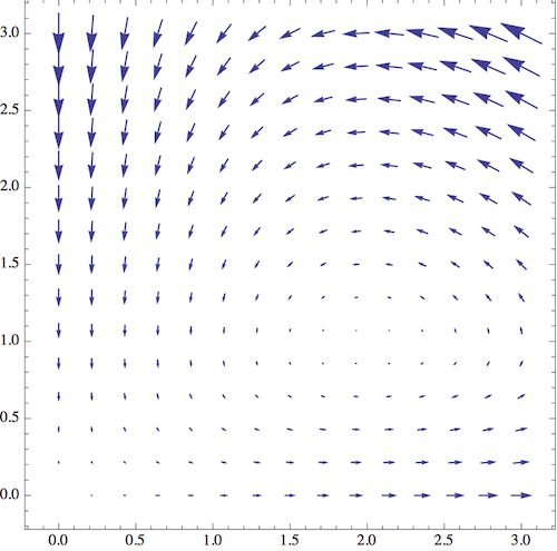
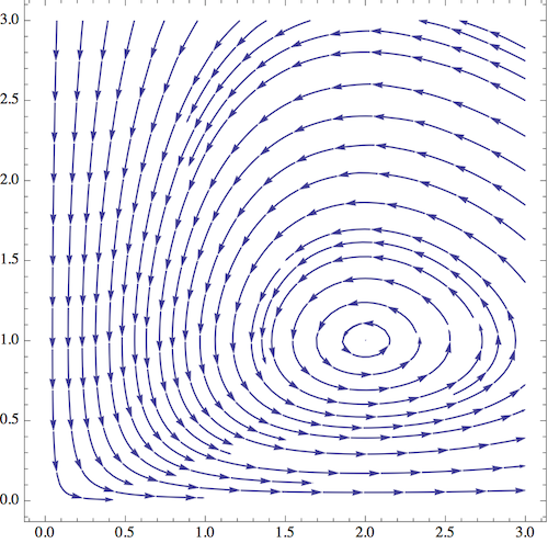
This is a very revealing picture! First of all, close to the axes, the derivatives follow the behavior that we predicted; the number of foxes is driven to be very small, and then the number of rabbits becomes very large. But the more interesting part of the diagram is near the equilibrium point (2,1). If I start nearby and follow the vector field around, the system seems to exhibit periodic behavior; the state goes around the equilibrium point in a closed loop. (If I draw the diagram very carefully, say by solving numerically with a computer, I find that the loops are indeed closed.)
We can take one of these curves and draw what is happening to R and F separately, and we get something like this, say for a starting point of (R,F) = (2,1/2):
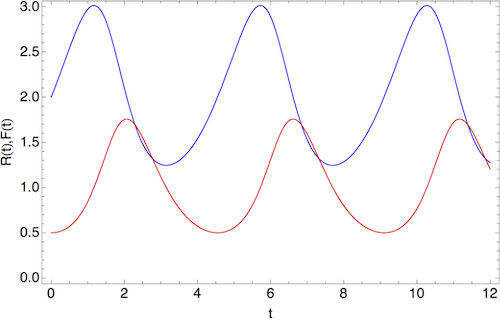
The population of rabbits is in blue, and that of foxes is in red. We see that the motion is periodic, although it’s not described by sines and cosines (for other choices of initial values, the exponential nature of the growth and decay would be more obvious.) Note also that the population peak of foxes comes after the peak in rabbits; this is characteristic behavior of the Lotka-Volterra model.
It shouldn’t surprise you to learn that there is actually a conserved quantity in this system, which does not change along any of these closed curves that we can draw. We can find it by noticing that if we multiply the first equation through by (c-dR)/R, and the second equation by (a-bF)/F, then the right-hand sides are equal and opposite, which means that \left( \frac{c}{R} - d \right) \dot{R} + \left( \frac{a}{F} - b \right) \dot{F} = 0. We can write this whole thing as one big time derivative: \frac{d}{dt} \left[ c \log R - dR + a \log F - bF \right] = 0. The quantity in brackets, which we call V, is then always conserved: dV/dt = 0. So we can label any of the “orbits” we’ve seen by their values of V. If we had done things in the opposite order, the existence of a conserved V would let us predict the closed curves we’ve been drawing (we can draw them parametrically in x and y.)
Despite the fact that we can’t write down an analytic solution, we can say a lot about the behavior of the Lotka-Volterra model, especially by drawing diagrams showing the orbits of the system. We’ll make use of the same sorts of techniques to study physical systems; they will be particularly useful for the study of chaotic motion. But first we need to introduce some new formalism, that of Hamiltonian dynamics.
14.7 Worked examples
14.7.1 Example: the simplest coupled oscillator
Let’s return to the simple 3-mass coupled harmonic oscillator and try finding a solution.
We’ll take the simplest case where all masses and springs are identical: k_1 = k_2 = k_3 = k \\ m_1 = m_2 = m. The spring constant matrix then becomes \overset{\leftrightarrow}{K} = \left( \begin{array}{cc} 2k & -k \\ -k & 2k \end{array} \right) so the matrix appearing in the eigenvalue equation is \overset{\leftrightarrow}{K} - \omega^2 \overset{\leftrightarrow}{M} = \left( \begin{array}{cc} 2k - m\omega^2 & -k \\ -k & 2k - m\omega^2 \end{array} \right). What are the squared normal frequencies? Taking the determinant, we have \det(\overset{\leftrightarrow}{K} - \omega^2 \overset{\leftrightarrow}{M}) = (2k-m\omega^2)^2 - k^2 \\ = 4k^2 + m^2 \omega^4 - 4km\omega^2 - k^2 \\ = 3k^2 - 4km\omega^2 + m^2 \omega^4 This looks like it will factorize, and the coefficients of k should be 1 and 3. Since the cross-term coefficient is -1-3, we can see that the factorized product is (k-m\omega^2)(3k-m\omega^2) so the two solutions are \omega^2 = +k/m, +3k/m.
Let’s press on and find the normal modes. For the small frequency \omega_a = \sqrt{k/m}, plugging back in gives us \overset{\leftrightarrow}{K} - \omega_a^2 \overset{\leftrightarrow}{M} = \left( \begin{array}{cc} k & -k \\ -k & k \end{array} \right). so the normal mode must satisfy \left( \begin{array}{cc} k & -k \\ -k & k \end{array} \right) \left( \begin{array}{c} A_1 \\ A_2 \end{array} \right) = 0. The solution to this equation is fairly obvious: the two amplitudes must be equal, A_1 = A_2 = A. Switching the time-dependenence back on, we can write \vec{x}_a = \left( \begin{array}{c} x_1(t) \\ x_2(t) \end{array} \right) = \left(\begin{array}{c} A \cos (\omega_a t - \delta) \\ A \cos (\omega_a t - \delta) \end{array} \right) = \left( \begin{array}{c} 1 \\ 1 \end{array} \right) A \cos (\omega_a t - \delta)\\ = \vec{v}_a A \cos (\omega_a t - \delta). where I’ve introduced the constant vector \vec{v}_a, which defines the “direction” of the normal-mode oscillation. Usually when we use the term “normal mode”, we’ll be referring to these vectors, which can be separated out from the harmonic oscillator part.
For the other frequency \omega_b = \sqrt{3k/m}, I won’t do the derivation on the board, but it’s easy to see that the second normal mode is \vec{v}_b = \left( \begin{array}{c} 1 \\ -1 \end{array} \right). (Notice that unlike the principal axes of rigid bodies, we don’t care about the normalization of these vectors, since it can be absorbed into the amplitude A of our harmonic oscillator solution.)
We can combine the two specific solutions into our general solution: \vec{x}(t) = \vec{x}_a(t) + \vec{x}_b(t) \\ = \left( \begin{array}{c} 1 \\ 1 \end{array} \right) A \cos \left( \sqrt{\frac{k}{m}} t - \delta_a \right) + \left( \begin{array}{c} 1 \\ -1 \end{array} \right) B \cos \left( \sqrt{\frac{3k}{m}} t - \delta_b \right). Note that we have four unknown quantities (A, B, \delta_a, \delta_b), which is exactly what we expect: for a second-order differential equation, we need 2 initial conditions (e.g. position and speed at t=0) for each of our 2 objects, so 4 initial conditions in all.
Physically, it’s fairly easy to see what’s going on here. The first normal mode corresponds to the two masses moving together; the distance between them stays fixed. In the other mode, they move at the same frequency and amplitude, but exactly out of phase, stretching and squeezing the middle spring.
14.7.2 Example: springs on a ring
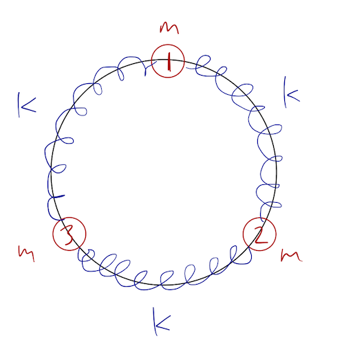
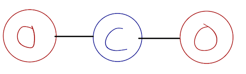
Here’s another example which will show some unique features that appear in certain versions of the coupled oscillator problem. We consider three identical masses m arranged on a ring, and connected by three identical springs with force constant k:
The kinetic energy is easy here: T = \frac{1}{2} mR^2 (\dot{\phi}_1^2 + \dot{\phi}_2^2 + \dot{\phi}_3^2) As for the potential, the length of the arc between any two springs is R (\phi_i - \phi_j). Angles are a little tricky, though, since there are factors of 2\pi floating around: if \phi_1 = 0.1 and \phi_3 = 2\pi - 0.1, for example, they’re actually fairly close together. It’s better to use displacements from equilibrium as usual: \beta_1 = \phi_1 \\ \beta_2 = \phi_2 - 2\pi / 3 \\ \beta_3 = \phi_3 - 4\pi / 3 Mathematically we should restrict what values these things can take on, but we know physically the springs will prevent anything too strange (e.g. the masses passing through each other) from happening, so we’ll just go ahead and solve in these coordinates. The potential is U = \frac{1}{2} kR^2 \left( (\beta_2 - \beta_1)^2 + (\beta_3 - \beta_2)^2 + (\beta_1 - \beta_3)^2 \right) We have three equations of motion to find. Let’s start with \beta_1: \frac{\partial \mathcal{L}}{\partial \beta_1} = \frac{d}{dt} \left( \frac{\partial \mathcal{L}}{\partial \dot{\beta}_1} \right) \\ -kR^2 (2\beta_1 - \beta_2 - \beta_3) = m R^2 \ddot{\beta}_1. Since the Lagrangian is totally symmetric between the three \beta_i, it’s easy to see that the other two equations look more or less the same, i.e. -k (-\beta_1 + 2\beta_2 - \beta_3) = m \ddot{\beta}_2 \\ -k (-\beta_1 - \beta_2 + 2\beta_3) = m \ddot{\beta}_3. where all the R^2 factors cancel out. From here, we read off the two matrices. \mathbf{K} = \left( \begin{array}{ccc} 2k & -k & -k \\ -k & 2k & -k \\ -k & -k & 2k \end{array} \right) and \mathbf{M} = \left( \begin{array}{ccc} m & 0 & 0 \\ 0 & m & 0 \\ 0 & 0 & m \end{array} \right), so our eigenvalue equation is \left| \begin{array}{ccc} 2k-\omega^2 m & -k & -k \\ -k & 2k - \omega^2 m & -k \\ -k & -k & 2k - \omega^2 m \end{array} \right| = 0. I won’t go through the gory details on the board, but the result of this determinant is m^3 \omega^2 \left(\omega^4 - 6(k/m) \omega^2 + 9(k/m)^2 \right) = 0. The cubic nicely factorizes for us, so one eigenvalue is just \omega_1 = 0. For the other two, we solve the quadratic: \omega^2 = \frac{1}{2} \left[ \frac{6k}{m} \pm \sqrt{\frac{36k^2}{m^2} - 4 \frac{9k^2}{m^2}} \right] \\ = \frac{3k}{m}. Yes, only one solution, so \omega_2^2 = \omega_3^2 = 3k/m.
Now, what are the normal modes for each of these frequencies? We’ll start with \omega_1 = 0: plugging back into the eigenvalue problem matrix, \left( \begin{array}{ccc} 2k & -k & -k \\ -k & 2k & -k \\ -k & -k & 2k \end{array} \right) \left( \begin{array}{c} \xi_x \\ \xi_y \\ \xi_z \end{array} \right) = 0 This is straightforward to row-reduce, but you may also be able to spot immediately that the vector which solves all three equations is simply \vec{\xi}_1 = \left( \begin{array}{c} 1 \\ 1 \\ 1 \end{array} \right). This corresponds to equal displacement of all three masses in the same direction. But this can’t be a normal periodic motion, because the frequency is zero. If we remember that we’re solving for the acceleration, then zero frequency is just the differential equation \ddot{\vec{x}} = 0, i.e. movement with constant velocity.
Physically, we see that this is totally reasonable: if all three masses move with constant speed around the ring in the same direction, then the springs are never stretched, and there are no forces!
A zero mode is a solution to the coupled oscillator equation with \omega = 0. Since \omega = 0 in the differential equation \ddot{\vec{x}} = -\omega^2 \vec{x} corresponds to motion with constant velocity, a zero mode is a direction in which the system can drift freely without restoring force. For example, in the motion of two blocks coupled by a single spring (with no other forces), the motion of the center of mass of the two blocks is a zero mode.
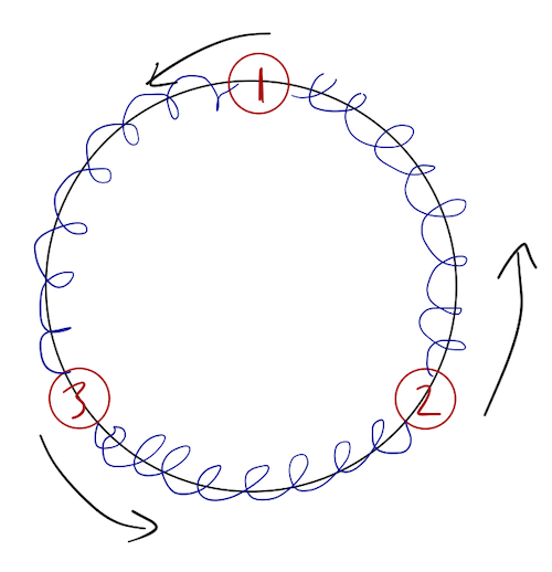
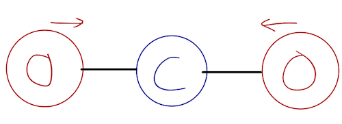
Now, what about the other normal modes? Since we have degenerate eigenvalues, we expect some ambiguity in finding them. The eigenvector equation with \omega^2 = 3k/m is \left( \begin{array}{ccc} -k & -k & -k \\ -k & -k & -k \\ -k & -k & -k \end{array} \right) \left( \begin{array}{c} \xi_x \\ \xi_y \\ \xi_z \end{array} \right) = 0 No row reduction necessary! This is the same equation repeated three times, namely \xi_x + \xi_y + \xi_z = 0, which is (of course) just the condition that these other normal modes are both orthogonal to the first one we found (the zero mode.) As always in this situation, we’re free to pick any two orthogonal vectors that satisfy this condition, let’s say \vec{\xi}_2 = \left( \begin{array}{c} 1 \\ -1 \\ 0 \end{array} \right) \\ \vec{\xi}_3 = \left( \begin{array}{c} 1 \\ 0 \\ -1 \end{array} \right) So the second mode corresponds to masses 1 and 2 oscillating back and forth, while mass 3 is stationary:
The third mode is the same thing, but with masses 1 and 3 oscillating and mass 2 fixed.
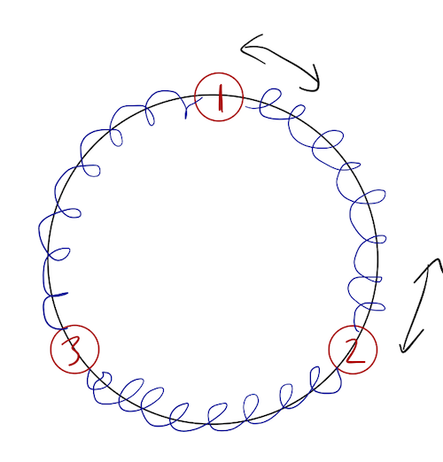
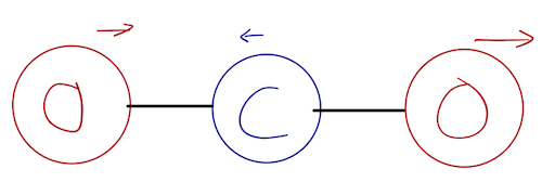
Of course, this problem is very symmetric, so we should ask: what about the possibility of mass 1 being fixed while 2 and 3 oscillating? That “direction” is just a difference of the other two modes, i.e. \vec{\xi}_2 - \vec{\xi}_3 = \left( \begin{array}{c} 0 \\ -1 \\ 1 \end{array} \right). Ordinarily this would be a combination of two different oscillations, but because \vec{\xi}_2 and \vec{\xi}_3 have the same normal frequency, this combination is also simply a normal mode. It’s easier to see what’s happening if we write the general solution out: \vec{\phi}(t) = A_0 + B_0 t + A_1 \left( \begin{array}{c} 1 \\ -1 \\ 0 \end{array} \right) \cos (\sqrt{3k/m} t + \delta_1) + A_2 \left( \begin{array}{c} 1 \\ 0 \\ -1 \end{array} \right) \cos (\sqrt{3k/m} t + \delta_2) Since the latter two terms have the same frequency, we can combine them and end up with an oscillation proportional to another vector, just with a different amplitude and phase. The only restriction is that the resulting vector always satisfies \xi_x + \xi_y + \xi_z = 0.
In the end, the motion of this system isn’t too interesting: all possible motions of the springs are combinations of zero-mode motion, and some oscillation at the fixed frequency \omega = \sqrt{3k/m}, such that the positions of the three masses always satisfy \beta_1 + \beta_2 + \beta_3 = 0. If we changed one of the masses or spring constants, in general we’d find three distinct normal modes and more complicated motion. (The zero-mode will always remain, no matter what.)
14.7.3 Example: the double pendulum
For the most part, there’s not too much difficulty in expanding the framework we’ve needed to bigger and more complex systems. Certainly a big collection of carts and springs won’t make things more interesting; it will just force us to deal with bigger matrices. But it’s worth looking at some coupled oscillators that aren’t just springs and masses, to illustrate some more general features. So let’s consider the double pendulum:
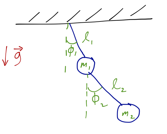
We’ve thought about setting up the Lagrangian for this system before. Starting with the potential energy, for mass 1 we simply have U_1 = m_1 g \ell_1 (1 - \cos \phi_1) doing a bit of geometry and checking that the potential is smallest (zero, in these coordinates) at \phi_1 = 0. The potential energy of mass 2 is similar, except that we have to add the vertical position of the first mass as well: U_2 = m_2 g [\ell_1 (1 - \cos \phi_1) + \ell_2 (1 - \cos \phi_2)]. As for the kinetic energy, we can think of it in terms of vectors. Because mass 1 only moves by changing \phi_1, its velocity vector points in the \hat{\phi}_1 direction: \vec{v}_1 = \ell_1 \dot{\phi}_1 \hat{\phi}_1 so T_1 = \frac{1}{2} m_1 v_1^2 = \frac{1}{2} m_1 \ell_1^2 \dot{\phi}_1^2. Of course, I didn’t need to write this as a vector; we know that this is what the kinetic energy of rotation about a point at fixed distance \ell_1 looks like. But mass 2 has a more complicated kinetic term; its position depends on the position of mass 1 as well.
Since we’ve set this up in terms of velocity vectors, all we need to do is square our expression for \vec{v}_2, which is \vec{v}_2 = \ell_1 \dot{\phi}_1 \hat{\phi}_1 + \ell_2 \dot{\phi}_2 \hat{\phi}_2 Then |\vec{v}_2|^2 = \vec{v}_2 \cdot \vec{v}_2 = \ell_1^2 \dot{\phi}_1^2 + \ell_2^2 \dot{\phi}_2^2 + 2 \ell_1 \ell_2 \dot{\phi}_1 \dot{\phi}_2 (\hat{\phi}_1 \cdot \hat{\phi}_2). The dot product of the two unit vectors is equal to the cosine of the angle between them, which is (\phi_2 - \phi_1).
At this point, I’m going to set m_1 = m_2 = m and \ell_1 = \ell_2 = \ell, just to make things simpler to work through. Doing so, our total Lagrangian for this system from the pieces we have found is \mathcal{L} = m \ell^2 \dot{\phi}_1^2 + \frac{1}{2} m \ell^2 \dot{\phi}_2^2 + m \ell^2 \dot{\phi}_1 \dot{\phi}_2 \cos(\phi_1 - \phi_2) \\ \ + mg \ell \left( 2\cos \phi_1 + \cos \phi_2 \right) We can go on to write the equations of motion, but it’s clear we won’t be able to write it in the linear form that we used to solve the coupled mass and spring system, because of the cosines. But we know how to deal with the cosines already, from studying a single pendulum: we make a small-angle approximation. We’ll keep terms up to order \phi^2 or \dot{\phi}^2 in the Lagrangian, to end up with terms of order \phi after taking derivatives to find the equations of motion. Thus, using \cos(x) \approx 1 - \frac{x^2}{2}, we find the approximate result \mathcal{L} \approx m\ell^2 \dot{\phi}_1^2 + \frac{1}{2} m\ell^2 \dot{\phi}_2^2 + m \ell^2 \dot{\phi}_1 \dot{\phi}_2 - \frac{1}{2} mg \ell (2 \phi_1^2 + \phi_2^2). Now we can differentiate: \frac{\partial \mathcal{L}}{\partial \phi_1} = \frac{d}{dt} \frac{\partial \mathcal{L}}{\partial \dot{\phi}_1} \\ -2mg\ell \phi_1 = 2m\ell^2 \ddot{\phi}_1 + m\ell^2 \ddot{\phi}_2 \\ -mg\ell \phi_2 = m\ell^2 \ddot{\phi}_2 + m\ell^2 \ddot{\phi}_1. We can write this in the usual matrix form, \overset{\leftrightarrow}{M} \ddot{\vec{\phi}} = -\overset{\leftrightarrow}{K} \vec{\phi}, except now M is the more complicated matrix: \overset{\leftrightarrow}{M} = m\ell^2 \left( \begin{array}{cc} 2 & 1 \\ 1 & 1 \end{array} \right) \\ \overset{\leftrightarrow}{K} = -m\ell^2 \left( \begin{array}{cc} 2\omega_0^2 & 0 \\ 0 & \omega_0^2 \end{array} \right) where for convenience, I’ve defined the constant \omega_0 = \sqrt{g/\ell}, which you’ll recognize as the usual frequency for small oscillations of a pendulum. Cancelling the common factor of m\ell^2, we can then write the combined matrix for the generalized eigenvalue problem as \overset{\leftrightarrow}{K} - \omega^2 \overset{\leftrightarrow}{M} = \left( \begin{array}{cc} 2 (\omega_0^2 - \omega^2) & -\omega^2 \\ -\omega^2 & (\omega_0^2 - \omega^2) \end{array} \right) which has determinant \det(\overset{\leftrightarrow}{K} - \omega^2 \overset{\leftrightarrow}{M}) = 2(\omega_0^2 - \omega^2)^2 - \omega^4 = 0 \\ \omega^4 - 4 \omega_0^2 \omega^2 + 2\omega_0^2 = 0. This is just a simple quadratic equation, and the roots are \omega^2 = \omega_0^2 (2 \pm \sqrt{2}). As always, we plug back in to find the eigenvectors; I’ll skip the details, but you can verify that the result we get is \omega_1^2 = \omega_0^2 (2 - \sqrt{2}), \hat{\xi}_1 = \frac{1}{\sqrt{3}}\left(\begin{array}{c} 1 \\ \sqrt{2} \end{array} \right) \\ \omega_2^2 = \omega_0^2 (2 + \sqrt{2}), \hat{\xi}_2 = \frac{1}{\sqrt{3}} \left(\begin{array}{c} 1 \\ -\sqrt{2} \end{array} \right). and as usual, the general solution is given by combining the two, \vec{\phi}(t) = A_1 \hat{\xi}_1 \cos (\omega_1 t - \delta_1) + A_2 \hat{\xi}_2 \cos (\omega_2 t - \delta_2) \\ = \left(\begin{array}{c} A_1 \cos (\omega_1 t - \delta_1) + A_2 \cos(\omega_2 t - \delta_2) \\ \sqrt{2} A_1 \cos (\omega_1 t - \delta_1) - \sqrt{2} A_2 \cos (\omega_2 t - \delta_2) \end{array} \right). What does motion in each of the normal modes look like? For the first mode (A_2 = 0), the two masses oscillate completely in phase, but the amplitude (in \phi_2) of the lower component is larger by a factor of \sqrt{2} (so it will swing out further.) In the second mode, the amplitudes are the same, but the motion is 180^{\circ} out of phase; they swing in opposite directions.
14.7.4 Example: vibrational energy of carbon dioxide
Here’s a system that you probably didn’t think you’d see in classical mechanics: a carbon dioxide molecule.
CO2 is a nice molecule to deal with, because the atoms are arranged more or less in a straight line. Molecules can exist in what are called excited states, where they have extra energy stored inside them; vibrational motion is one example of how this energy can be stored.
There are a few different ways that a CO2 molecule can vibrate, but let’s focus on just one-dimensional motion in the direction along the molecule. Let’s take m_O to be the mass of oxygen, and m_C the mass of carbon. In terms of the coordinates shown, we know that \mathcal{L} = \frac{1}{2} m_O\dot{x_1}^2 + \frac{1}{2} m_C\dot{x_2}^2 + \frac{1}{2} m_O\dot{x_3}^2 - V(x_1 - x_2) - V(x_2 - x_3). The potential V(r) corresponds to the interatomic binding energy, and in general is quite complicated. But we don’t need to know its form to study small vibrations! The equilibrium point, given by the minimum-energy state, we take to be |x_1 - x_2| = r_0. By symmetry, |x_2 - x_3| = r_0 at equilibrium as well. As above, we expand in small displacements \eta: x_i(t) = x_i^0 + \eta_i(t) By doing so, we can Taylor expand the unknown potential energy functions: V(r) = V(r_0) + \left. \frac{\partial V}{\partial r}\right|_{r=r_0} (r-r_0) + \frac{1}{2} \left.\frac{\partial^2 V}{\partial r^2} \right|_{r=r_0} (r-r_0)^2 + ... The first term is just a constant, which we can drop. Because r=r_0 is an equilibrium point, we know that \partial V / \partial r must vanish there (think back to central-force motion; stable equilibrium with no evolution happens when E = V at a minimum of the potential.) We have no idea what the second derivative is, but at r=r_0 it is just a constant, which we’ll call k: \left.\frac{\partial^2 V}{\partial r^2}\right|_{r=r_0} \equiv k. With that, we can substitute back in to find the potential energies in terms of the \eta’s: V(x_1 - x_2) \approx \frac{k}{2} (x_1 - x_2 - r_0)^2 = \frac{k}{2} (\eta_1 - \eta_2)^2 \\ V(x_2 - x_3) \approx \frac{k}{2} (\eta_2 - \eta_3)^2 so the Lagrangian for the \eta’s is \mathcal{L} \approx \frac{1}{2} m_O (\dot{\eta_1}^2 + \dot{\eta_3}^2) + \frac{1}{2} m_C \dot{\eta_2}^2 - \frac{k}{2} \left[ (\eta_1 - \eta_2)^2 + (\eta_2 - \eta_3)^2 \right]. Taking the appropriate derivatives, the Euler-Lagrange equations of motion are then m_O \ddot{\eta_1} = -k(\eta_1 - \eta_2) \\ m_C \ddot{\eta_2} = -k(\eta_2 - \eta_1) - k (\eta_2 - \eta_3) \\ m_O \ddot{\eta_3} = -k(\eta_3 - \eta_2). Dividing through by the masses and rewriting as a matrix, we have \ddot{\vec{\eta}} = -\overset{\leftrightarrow}{F} \vec{\eta} where \overset{\leftrightarrow}{F} = \left( \begin{array}{ccc} k/m_O & -k/m_O & 0 \\ -k/m_C & 2k/m_C & -k/m_C \\ 0 & -k/m_O & k/m_O \end{array} \right) (Notice, by the way, that F is not a symmetric matrix! Still, all the eigenvalues will be real; this is guaranteed by the fact that the individual matrices M and K arising from the kinetic and potential energy are symmetric.)
As always, to solve for the motion, we find the eigenvalues and eigenvectors of this matrix. Defining (k/m_O) \lambda^2 = \omega^2 and \rho \equiv m_O/m_C, the matrix we need for the eigenvalue problem is \overset{\leftrightarrow}{F} - \omega^2 \overset{\leftrightarrow}{I} = \frac{k}{m_O} \left( \begin{array}{ccc} 1-\lambda^2 & -1 & 0 \\ -\rho & 2\rho - \lambda^2 & -\rho \\ 0 & -1 & 1-\lambda^2 \end{array} \right) The characteristic equation is \det(\overset{\leftrightarrow}{F} - \omega^2 \overset{\leftrightarrow}{I}) = -(1-\lambda^2) [(2\rho - \lambda^2) (1-\lambda^2) - \rho] - \rho (1-\lambda^2) \\ = -(1-\lambda^2) \left [ \lambda^4 - (1 + 2\rho) \lambda^2 \right]. We can just read off the eigenvalues, since this is already nicely factorized: \omega_1 = \sqrt{k/m_O} \lambda_1 = 0 \\ \omega_2 = \sqrt{k/m_O} \lambda_2 = \sqrt{k/m_O} \\ \omega_3 = \sqrt{k/m_O} \lambda_3 = \sqrt{k/m_O (1 + 2m_O/m_C)}. If we solve for the eigenvectors, we find the range of motion we would expect: the first eigenvector is \vec{\xi}_1 = (1,1,1), corresponding to translation in space; there is no vibration at all, which we identify as a zero mode since \omega_1 = 0. The second and third modes are \vec{\xi}_2 = (1,0,-1) and \vec{\xi}_3 = (1,-2m_O/m_C, 1), corresponding to vibration of the oxygen atoms with C fixed (the symmetric stretch mode), and motion where the two oxygen atoms go one way and the carbon moves back the other way (the asymmetric stretch mode.)
Since we have no idea what k is here, we can’t calculate the normal frequencies directly. However, we can easily look at the ratio between the two stretch mode frequencies: \frac{\omega_3}{\omega_2} = \sqrt{1 + 2m_O / m_C} \approx 1.91. From basic quantum mechanics, we know that the energy associated with a particular frequency of vibration is E = \hbar \omega, so this should also give the ratio of the observed energies of these vibrations. Experimentally, we can measure this directly by looking for light emitted when the CO2 transitions from the higher-energy to lower-energy vibrational mode. The real measured ratio of energies for the antisymmetric to symmetric stretch modes is about E_3 / E_2 \sim 1.69, so our estimate is about 13% too high. Not too bad for doing classical mechanics on a quantum system!
(In fact, we could do better; one of the main problems with our estimate is that when we diagonalized we ignored the other important vibrational mode, “bending”, in which the C moves up and down with respect to the O atoms. But solving in two dimensions means we need a 6x6 matrix, and we know we need quantum mechanics to properly understand this molecule anyway, so let’s just move on.)