8 Calculus of variations and Lagrangian mechanics
As we have seen many times, in physics there is often more than one way to solve a problem. While Newton’s laws provide the foundation for all of classical mechanics, in some situations we can make use of conservation of momentum or energy to find a shorter way to obtain the same results.
A much more radical approach is to reformulate the theory of mechanics completely: provide a different framework that completely contains the same physics as Newton’s laws. We will be led to such a reformulation by asking a seemingly simple question about blocks on ramps.
8.1 Warm-up: block on a ramp
Let’s remind ourselves about a classic and simple example: the block on an inclined plane.
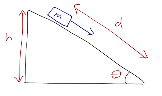
A block of mass m sits on a frictionless plane, inclined at angle \theta. The block starts at rest with initial height h, with d the displacement along the ramp from its starting point (so d = h / \sin \theta is the bottom of the ramp.) How long does it take to reach the bottom of the ramp?
We know how to solve this using free-body diagrams, but also the quick way using conservation of energy, which is what I’ll focus on for now. We know that the change in kinetic energy \Delta T equals minus the change in potential, \Delta T = \Delta U. Starting from rest and letting v_f be the final speed, then, we have (0 - \frac{1}{2} mv_f^2) = (mgh - 0) \\ v_f = \sqrt{2gh} Then, knowing that the block is experiencing constant acceleration, we know that v = at, so d = \frac{1}{2} at_f^2 = \frac{1}{2} v_f t_f, and therefore t_f = 2d / v_f = \frac{2(h/\sin \theta)}{\sqrt{2gh}} = \sqrt{\frac{2h}{g}} \frac{1}{\sin \theta}. Note that we can’t only use conservation of energy; we needed to make an assumption about the forces to know the acceleration was constant in order to get the answer for t_f. I could have drawn any arbitrary shape for the ramp, and we still know v_f, but to find the time taken we need to know the entire history of what the block did on its way down.
Of course, nothing is stopping us from solving this problem using Newton’s laws, except that it will be quite complicated to keep track of the normal force along the ramp, since its direction is changing constantly. It would be great if we had a more general energy-based method, which would eliminate the need to keep track of such forces…
8.1.1 The brachistochrone problem
Let’s be even more general than just having a specific weirdly-shaped ramp. Suppose that instead of giving you a ramp, I give you the details of the block and the initial and final positions, and ask you to build a ramp which will minimize t_f. How can you do it? (This is actually an old and famous problem in mechanics called the brachistochrone problem - Greek for “short time”.)
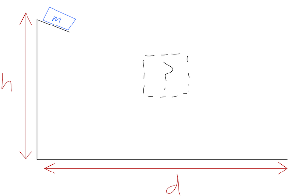
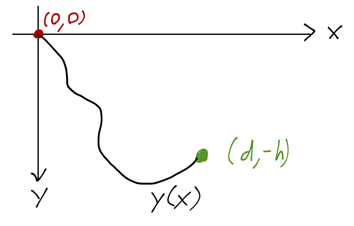
Let’s be concrete: we can keep track of the position of our block as y(t), and we’re given the two conditions y(0) = 0 \\ y(d) = -h. The shape of the ramp is some arbitrary function which we can write as y = f(x). Our only assumption will be that the ramp is well-behaved enough that the block doesn’t get stuck somewhere in the middle before reaching x=d.
The good news is that because this problem has only conservative forces, we can actually still use conservation of energy to solve it! We just have to be careful to account for the (unknown) shape of the ramp. At any instant, we know that T + U = 0 (since y(0)=0), or T + U = 0 \\ \frac{1}{2} m (\dot{x}^2 + \dot{y}^2) + mgy = 0 Notice that although the presence of the ramp means that we don’t have to keep track of x and y independently, the speed of the block still depends on both coordinates! We can rewrite: \dot{y} = \frac{dy}{dt} \\ = \frac{dy}{dx} \frac{dx}{dt} \\ = f'(x) \dot{x} where y' = df/dx. Plugging back in above and rearranging: -2gy = \dot{x}^2 \left(1 + f'(x)^2 \right) \\ 1 = \frac{dx}{dt} \sqrt{ \frac{1+f'(x)^2}{-2gf(x)}} \\ t[f] = \int dt = \int_0^d dx \sqrt{ \frac{1+f'(x)^2}{-2gf(x)}}. That’s our answer: given an arbitrary f(x), we can do the integral (at least numerically) to find the time taken for the block to reach the bottom. But we still haven’t answered the main question: which f(x) will give us the optimal (i.e. fastest) t?
This is an example of an optimization problem, and we recall from calculus how to deal with them: the extreme (maximum and minimum) values of any function f(x) are found where its derivative vanishes. But t isn’t a function of one variable, or even of a list of variables; it’s a function of a function, f(x). Such an object is known as a functional.
A quick aside on a trick that I did above: I “split the derivative” by separating dx/dt and putting dt on the left side of the equation before integrating. This is something of an abuse of notation, although it’s actually simple and rigorous if you don’t skip steps. (If you are happy with Leibniz notation, i.e. thinking of separate “infinitesimals” dx and dt, then splitting them apart is fine on its own.)
Here’s how it works: if we have \frac{dx}{dt} f(x) = g(t) then we first integrate both sides with respect to t, \int dt\ \frac{dx}{dt} f(x) = \int dt\ g(t). Now we just need to do a u-substitution on the left integral: if we change from dt to dx, then \int \left[dx \frac{dt}{dx}\right] \frac{dx}{dt} f(x) = \int dt\ g(t), and we can cancel off dx/dt and its reciprocal, leaving the expression we would get from just splitting the derivative up, \int dx\ f(x) = \int dt\ g(t).
8.2 Functionals
Just like a function is a map which takes some numbers as inputs and gives us a single number as output, a functional is a map from a function to a single number. Our solution to the ramp above is a functional: t[f] takes a function (the shape of the ramp) as input, and gives us a number (how long it takes to reach the bottom) as output.
Another very familiar functional is curve length, usually written S. If we imagine drawing curves y(x) in the x-y plane, then for any such curve we can assign a length. If we break the curve down into infinitesimal pieces ds, then we can write S as an integral: S[y] = \int_{y(x)} ds = \int_{y(x)} \sqrt{dx^2 + dy^2} \\ = \int dx\ \sqrt{1 + y'(x)^2} where y'(x) \equiv dy/dx.
(A brief note on notation: sometimes I like to put the dx on the left side of the integral, instead of the right. It means the same thing, not an integral times a function outside of it. I’ll try to use brackets if things are ambiguous.)
For every problem we will study in this class, the most general functional J acting on a single space of functions \{y(x)\} can always be written as an integral of the form J[y] = \int dx\ F(x, y, y'), where F is an ordinary function and again y' = dy/dx. You can see that the examples we’ve studied so far both look like this. Now, you should be able to see where this is going: if we can define some version of a derivative on J[y], then maybe we can use it to solve the optimization problem.
8.2.1 Reminder: optimization in ordinary calculus
Before we do that, let’s go back to single-variable calculus and remind ourselves of some details. What is the connection between the derivative of a function and the extrema (minimum and maximum points) of that function?
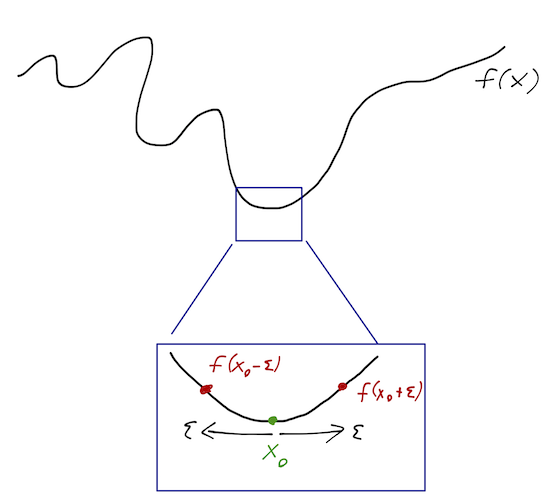
x_0 is a local minimum; if we move away from x_0 by some small displacement \epsilon, we find that f(x_0+\epsilon) \geq f(x_0), and f(x_0-\epsilon) \geq f(x_0). But now remember the definition of the derivative at x_0: f'(x_0) = \lim_{\epsilon \rightarrow 0} \frac{f(x_0 + \epsilon) - f(x_0)}{\epsilon} \geq 0 since the numerator is positive. But we can also flip the sign of \epsilon and we still get the derivative in the limit: f'(x_0) = \lim_{\epsilon \rightarrow 0} \frac{f(x_0 - \epsilon) - f(x_0)}{-\epsilon} \leq 0. The only way to satisfy both of these conditions is for the derivative to vanish! So f'(x_0) = 0. This is a necessary condition for a local minimum; in other words, if we have a minimum, the derivative is guaranteed to vanish at that point (same for a maximum.)
What we haven’t proven - and we know it isn’t true, so good thing! - is that f'(x_0) = 0 is a sufficient condition for a minimum or maximum, or in other words, that a zero derivative guarantees a minimum or maximum at that point. We know that the derivative also vanishes at saddle points, which are neither minima or maxima, like x_0 = 0 for the function f(x) = x^3.
You can prove the relation using the definition of a derivative, which is probably what you did in math class, but another way is to use a Taylor series expansion. (In physics class, Taylor expansion should be the first tool you reach for in a lot of situations!) This second approach won’t carry over directly to the calculus of variations, but it will help to give some intuition here.
Recall that a Taylor series about the point x_0 is an infinite sum of increasing powers of (x-x_0)^n. So if we’re very close to x_0, we can just keep the first few terms and throw the rest away. Let’s expand f(x_0 + \epsilon) about x_0: f(x_0 + \epsilon) = f(x_0) + \epsilon f'(x_0) + \frac{1}{2} \epsilon^2 f''(x_0) + ... Start by looking at the first term, \epsilon f'(x_0), which is linear in \epsilon. This tells you if you zoom in far enough, the function f(x) itself looks linear at the point x_0. But that means that f(x) increases in one direction, and decreases in the other - it can’t be an extreme value! f(x_0 + \epsilon) \approx f(x_0) + \epsilon f'(x_0) \\ f(x_0 - \epsilon) \approx f(x_0) - \epsilon f'(x_0) The only way out is for this term to vanish, so once again we’re led to the necessary condition f'(x_0) = 0.
Now suppose the first term is zero, and look at the second term. This term is quadratic in \epsilon - locally, f(x) looks like a parabola. So the sign of f''(x_0) matters - it tells us whether the parabola opens up (minimum) or down (maximum). Hence, testing the sign of the second derivative lets us decide whether we have a minimum or maximum.
8.3 The Euler-Lagrange equation and variational methods
Now we move from extrema of ordinary functions to extrema of functionals. Another common functional optimization problem, beyond the brachistochrone, is finding the shortest distance between two points, which involves the path length S[y].
To define a functional, we also have to define the space of functions on which it acts. If we want to use S to ask the question “what is the shortest distance between point A and point B in the plane?”, then we would restrict \{y(x)\} to all functions y(x) that begin and end at those points. We had a similar restriction on the endpoints in our brachistochrone problem.
Let’s be explicit and do a quick, concrete comparison between “function” and “functional”. Take as an example the function y(x) = 3x^2. The simplest thing we can do with a function is to evaluate it, i.e. to ask the question “what is y(x) at x=1?” Optimization problems ask the more difficult question “at which value of x is y(x) [minimum/maximum]?”, which requires us to evaluate y'(x) and solve for where it vanishes (and to look at higher derivatives, usually.)
Now let’s look at the functional version of all of the above. We can define a simple functional as the area under a curve from 0 to 1: A[y(x)] = \int_0^1 dx\ y(x). We are implicitly fixing boundary conditions when we define this functional; there is some set of functions y(x) we’re willing to consider. Let’s say in this case we want to fix y(0) = 0 and y(1) = 3, so that 3x^2 is one example. Now, the simplest thing we can do with A is evaluate it at a specific function: “What is A[y(x)] with y(x) = 3x^2?” We can also optimize, i.e. “What is the function y(x) (with the given boundary conditions) which minimizes (or maximizes) A[y]?”
What does an extreme (minimum or maximum) function look like, given some functional? If y_0(x) is a minimum of A[y], we expect that if we “move away” from y_0(x) just a little bit, if we adjust some part of the curve, we will always find that our new y(x) satisfies A[y] > A[y_0].
8.3.1 The general problem, Euler’s equation
Okay, let’s get back to our more general variational problem setup, with the definition of our general functional J: J[y] = \int_a^b dx\ F(x, y, y'). To decide whether the functional J[y] is at an extremum for some given curve y_0(x), we need a sensible way to compare y_0(x) to “nearby” curves in the same class. How do we decide what “nearby” means for a curve? We can construct such a nearby curve like so: y(x) \equiv y_0(x) + \alpha \eta(x) where \alpha is a real number, and \eta(x) is some other smooth curve. So long as \eta(x) is well-behaved, we can always ensure y(x) is “near” to y_0(x) by making \alpha sufficiently small.
Note that implicit in writing J[y] is a choice of boundary conditions; the functional isn’t defined properly without them! This means that not only are we fixing the range of integration from x=a to x=b, but we’re only considering functions which satisfy some conditions y(a) = y_1 \\ y(b) = y_2 Fixing the endpoints is very important; it means that when we write the “nearby” function in the sketch as y(x) = y_0(x) + \alpha \eta(x), the difference between them satisfies \eta(a) = \eta(b) = 0. This will be important in our proof, and more generally it’s needed so that we have a well-defined problem to solve. (Going back to the path length, you can ask the question “what is the shortest curve between two points”, but the question “what is the shortest curve” doesn’t make much sense.) Here’s a sketch of our setup:
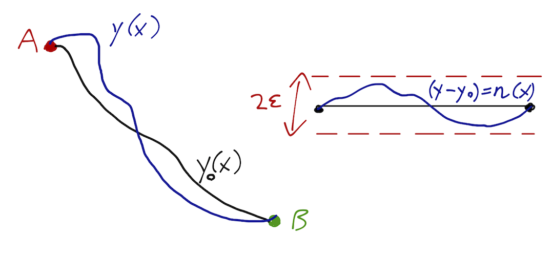
(Note that I’m not defining the quantity \epsilon, but if we want to be more careful mathematically we could - clearly by adjusting \alpha we can make the envelope \epsilon bounding the difference between functions arbitrarily small.)
We can expand out the functional value of this nearby curve: J[y] = \int_a^b dx\ F(x, y_0+\alpha \eta, y_0' + \alpha \eta') \\ \Delta J \equiv J[y] - J[y_0] = \int_a^b dx\ \left( F(x,y_0+\alpha \eta, y_0' + \alpha \eta') - F(x,y_0,y_0') \right). Because \alpha can be made infinitesimally small, we can Taylor expand F around our original function y_0. (If this seems like a suspicious thing to do, you can think about doing the expansion given a fixed value of x; since our argument will carry through no matter what x is, there’s no problem with applying Taylor’s theorem under the integral here.) Expanding to first order, we have for a multivariate function f(x+\epsilon,y) = f(x,y) + \epsilon \frac{\partial f}{\partial x}(x,y) + ... (which is just the one-variable version since we’re holding y fixed), so in the functional above, \Delta J = \int_a^b dx\ \left( \frac{\partial F}{\partial y} \alpha \eta(x) + \frac{\partial F}{\partial y'} \alpha \eta'(x) \right) \\ Just as for ordinary functions, it turns out that the condition for J[y_0] to be a minimum is that the infinitesimal difference between J[y_0] and the nearby curve J[y] should go to zero as \alpha does: \lim_{\alpha \rightarrow 0} \Delta J / \alpha = 0, or dJ/d\alpha = 0 if you prefer. The difference now is that we have an arbitrary function \eta(x) as well, and the difference should vanish for any choice of \eta.
Let’s try to simplify this: since \eta is arbitrary we don’t know how \eta and \eta' are related, but we can still integrate by parts to move the derivative off of \eta': \int_a^b dx\ \frac{\partial F}{\partial y'} \alpha \eta'(x) = \left.\alpha \eta(x) \frac{\partial F}{\partial y'}\right|_a^b - \int_a^b dx\ \alpha \eta(x) \frac{d}{dx} \left(\frac{\partial F}{\partial y'}\right). Importantly, the boundary term vanishes by construction, since \eta(a) = \eta(b) = 0! So we can combine the other two terms under the integral, which are now both proportional to \eta: \Delta J = \int_a^b dx\ \alpha \eta(x) \left[ \frac{\partial F}{\partial y} - \frac{d}{dx}\left(\frac{\partial F}{\partial y'}\right) \right]. Note that the connection to extreme values of J[y] is easy to see! If y_0 is a minimum of J[y], then we must have \Delta J \geq 0. But this first term is, in a sense, linear in the variation \eta(x). If the integral gives us any positive number, then the same integral with \eta \rightarrow -\eta will be negative, contradicting the statement that y_0 is a minimum. So the only possibility is that the integral vanishes.
This doesn’t mean that all of \Delta J vanishes; there are still higher-order terms, remember. But in many books you will see a special notation for this first term. Given a functional J[y], we write \delta J \equiv \int dx\ \delta y \left[\frac{\partial F}{\partial y} - \frac{d}{dx}\left(\frac{\partial F}{\partial y'}\right)\right]. \delta J is called the variation of the functional, and \delta y (which was \alpha \eta, but I’ve changed it to more conventional notation) is called the variation of the curve y(x). The condition for a minimum or maximum is then \delta J = 0. The variation \delta J is essentially the equivalent of the first derivative for a functional. You might be tempted to try to write the expression in square brackets as something like \delta J / \delta y, but remember that \delta y is a function of x; you can’t move it outside the integral. From the condition that \delta J = 0, which has to hold for any \delta y, we arrive at the celebrated Euler-Lagrange equation:
Any curve y that gives a stationary point of the functional J[y] = \int dx\ F(x,y,y') satisfies \frac{\partial F}{\partial y} - \frac{d}{d x}\left(\frac{\partial F}{\partial y'}\right) = 0.
(Sometimes written E-L for short.)
I’ve done all of this for only one dependent variable, but if we have more than one dependent variable y_1, y_2, ..., the functional becomes J = \int dx\ F(x, y_1, y_1', y_2, y_2', ...) and the total variation just becomes a sum over the same integral expression for each variable - in other words, we do the same derivation for one y at a time. Thus, the generalization to multiple dependent variables is just that we get a system of Euler-Lagrange equations instead, \frac{\partial F}{\partial y_i} - \frac{d}{dx}\left(\frac{\partial F}{\partial y_i'}\right) = 0. The book has some additional detail on this. This multiple-variable form will be extremely useful when we get back to mechanics, when we’ll want to keep track of complicated systems that have multiple objects with different coordinates.
8.3.2 Example: shortest distance between two points on a plane
Back to our shortest-distance problem. We wrote the curve-length functional already, S = \int_a^b dx\ \sqrt{1 + y'^2}. Taking derivatives of the integrand: \frac{\partial F}{\partial y} = 0, \\ \frac{\partial F}{\partial y'} = \frac{y'}{\sqrt{1+y'^2}}. The E-L equation is thus \frac{\partial}{\partial x}\left( \frac{y'}{\sqrt{1+y'^2}} \right) = 0. Expanding the derivative out would make life more complicated; instead we use the knowledge that the left-hand side is constant with respect to x, so y' = C\sqrt{1+y'^2} for some number C. Squaring and rearranging, this means that y'^2 = C^2 (1 + y'^2) \\ y'^2 = \frac{C^2}{1-C^2}. or y' = m, for some other constant m! This is a very simple differential equation, which we can solve by just integrating both sides, giving: y(x) = mx + c which is, of course, a straight line. We could now solve for m and c in terms of the endpoints by using the boundary conditions if we wanted.
Notice that our solution of the E-L equation simplified here, because F didn’t depend on y, just y'. For F independent of y', the E-L equation is even simpler - we just get \partial F / \partial y = 0. Finally, if F is independent of x, we can also write down a simplified version of the E-L equation (you’ll derive this in the homework): \frac{\partial F}{\partial x} = 0 \Rightarrow F - y' \frac{\partial F}{\partial y'} = \textrm{const.} This is sometimes called the second form of the Euler-Lagrange equation, and it can simplify certain problems.
8.3.3 Example: shortest distance between two points on a sphere
Let’s do a more interesting shortest-distance problem. (Math aside: the shortest distance connecting two points on a general surface is called a geodesic.) Obviously we should use spherical coordinates! If you start with ds = \sqrt{dx^2 + dy^2 + dz^2} and change coordinates, you will find: ds^2 = dr^2 + r^2 d\theta^2 + r^2 \sin^2 \theta d\phi^2. Letting R be the radius of the sphere, dr vanishes since we’re moving on the surface, and so S = \int \sqrt{R^2 d\theta^2 + R^2 \sin^2 \theta d\phi^2} \\ = R \int_{\theta_a}^{\theta_b} d\theta\ \sqrt{ 1 + \phi'(\theta)^2 \sin^2 \theta}. Since F(\theta, \phi, \phi') doesn’t depend on \phi, the Euler-Lagrange equation simplifies to \frac{\partial F}{\partial \phi'} = C \\ \frac{\sin^2 \theta\ \phi'}{\sqrt{1 + \sin^2 \theta\ \phi'^2}} = C. At this point we can solve for \phi' and then integrate over \theta, but finding the solution and then interpreting the result is sort of messy. Instead, we can exploit the symmetry of the sphere. We want the path from point A to point B, but we can rotate the sphere around to put point A where we want. The best place to put it is at the north pole, \theta_A = 0, which immediately gives us C = 0. But if C vanishes for the entire trajectory, then we must have \frac{d\phi}{d\theta}= 0. So the shortest path is a line of longitude, with the sphere rotated to this orientation. More generally, if we rotate the sphere again the path becomes a great circle, which is the intersection of a plane through the center of the sphere with the sphere itself.
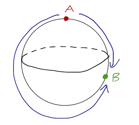
Notice that there are two paths satisfying the E-L equation, clockwise or counter-clockwise. (If you’re flying from Denver to New York, you can go east or west, for example.) The shorter path of the two is the true minimum distance.
Even in this relatively simple example, we had to worry about what sort of stationary points solving the Euler-Lagrange equation gave us! But don’t worry too much - for most physical problems we will deal with, the functional will have a minimum but no maximum value (just like the path length.) This means that in most situations the minimum solution will exist and be unique. For those special cases like the sphere where saddle points may also appear, we can figure out which one is the minimum just by testing which solution gives the smallest value of the functional.
8.4 The Lagrangian formalism
Now let’s go back and finally solve the problem that motivated the calculus of variations in the first place.
This solution is a little cumbersome, and requires a very non-obvious substitution to evaluate the integral near the end. Full details here for the curious.
Once again, the problem involves letting the shape of the ramp be arbitrary: we have to optimize over the time taken for the block to reach the bottom. As before I keep the height h and distance d to the final point fixed. In fact, let me fix a coordinate system: let’s take y(0) = 0 and y(d) = -h. We are interested in finding y(x) which minimizes the time for our block to reach the bottom. This is a very famous problem in physics, known as the brachistochrone (from the Greek words for “short time”.)
Since the ramp is frictionless, we know that v = \sqrt{-2gy} by conservation of energy. So, the time functional is: t = \int dt = \int \frac{ds}{v} \\ = \int \frac{\sqrt{dx^2 + dy^2}}{\sqrt{-2gy}} \\ = \int_{-h}^0 dy\ \sqrt{\frac{x'^2 + 1}{-2gy}}. We’ve used x as the dependent variable, so the E-L equation simplifies: \frac{\partial F}{\partial x'} = C = \frac{x'}{\sqrt{y(x'^2+1)}} \\ C^2 y (x'^2 + 1) = x'^2 \\ x'^2 = \frac{C^2 y}{1 - C^2 y} \\ \frac{dx}{dy} = \sqrt{\frac{y}{2a - y}} where a is a new constant that we’ve chosen to give a nice-looking final answer. We can do a sneaky substitution to integrate and solve this diff. eq! Let y = a(1 - \cos \theta), so that dy = d\theta\ a \sin \theta. Then the integral for x simplifies drastically: x = \int dy\ \frac{\sqrt{1 - \cos \theta}}{\sqrt{1+\cos \theta}} \\ = \int dy\ \frac{1-\cos \theta}{\sqrt{1-\cos^2 \theta}} \\ = \int (d\theta\ a \sin \theta) \frac{1-\cos \theta}{\sin \theta} \\ = a (\theta - \sin \theta) + x_0. So we now have a parametric solution for the path - x as above, and y(\theta) = a(1-\cos \theta). Since our boundary values for y are h and 0, we can identify x(\theta=0) = y(\theta=0) = 0, fixing x_0 = 0. At the other end, we have the system of equations x(\theta_f) = d = a(\theta_f - \sin \theta_f)\\ y(\theta_f) = -h = a(1-\cos \theta_f) Inverting for a and \theta_f is messy; for most cases, you can only do it numerically. However, we can draw the general parametric curve to give you some idea of what solutions look like in general:
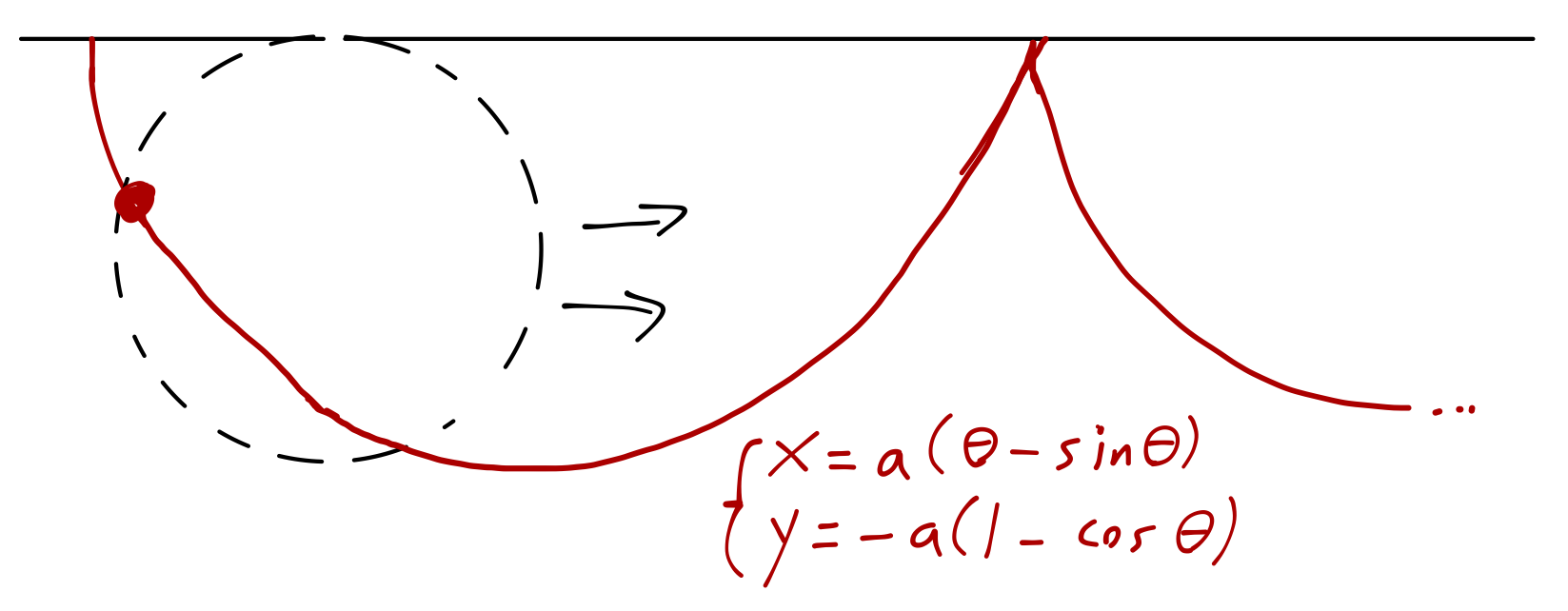
This curve is known as a cycloid (or sometimes as a brachistochrone) - it is the curve traced by point on a circle rolling along the x-axis. Note that depending on the values of d and h, the fastest path can actually overshoot and come back up to the endpoint.
The cycloid result seems a little counterintuitive, so it’s nice to see it in action. Unfortunately, when I’ve tried doing a demo of this in the past, it’s pretty hard to really see the outcome. Fortunately, the internet exists! Here’s a video of Adam Savage demonstrating a brachistochrone against a couple of other ramp shapes, and here’s the full video of its construction.
8.4.1 Back to classical mechanics: the Lagrangian
So, how does all of this relatively esoteric math about optimization problems help us to solve general problems in classical mechanics? If I take us all the way back to our starting example of the fixed ramp and the block:
there doesn’t appear to be anything to optimize here. With a complete initial condition as sketched here, we know that classical mechanics is deterministic; Newton’s laws will tell us how the system evolves at any instant in time, and the evolution of the system is completely fixed. How would calculus of variations even show up here?
Let’s try to look at the system in a different way. When we solve for the motion of the block, we are finding the function y(t) that describes its position as a function of time. (The presence of the ramp means if we know y, we know x too.) In a sense, then, we can think of the correct solution as a “path” through space and time:
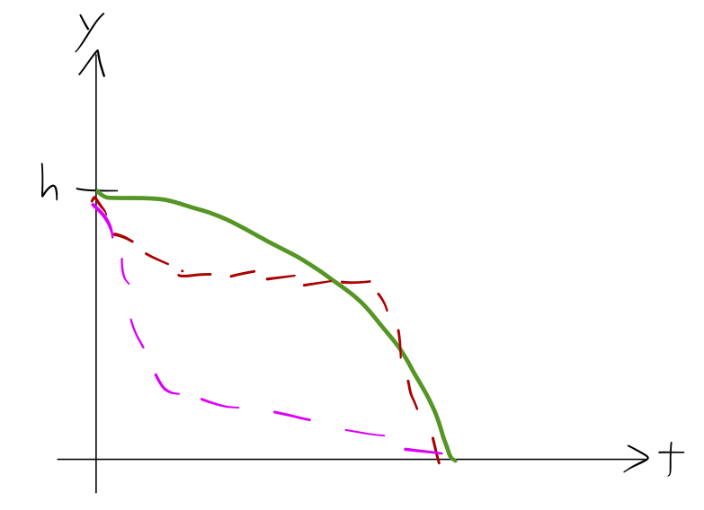
Newton’s laws tell us that the block will follow the solid path, and not any of the dotted ones: it won’t come to a stop and then start again, or accelerate rapidly and then move at constant speed. Our solution is a single “path” out of many possibilities we could have imagined. But if classical mechanics is really optimizing over paths like this, then what is the functional that’s being optimized?
Taylor just sort of throws the answer to this mystery at you, but in fact we can find a strong hint hidden in Newton’s laws if we stare at them long enough. Let’s see if we can guess the right functional to use, starting with a simple example, namely a single particle of mass m moving in one dimension x.
Newton’s second law is then F = m\ddot{x}. (Quick reminder of notation: dots are special notation for time derivatives, so \dot{x} = dx/dt, and \ddot{x} is the second derivative.)
To go further, we have to assume something about F. Recall from last semester that many forces are conservative, and that conservative forces have some nice properties. A conservative force is one which conserves mechanical energy: if a particle in a conservative force field comes back to where it started, no work will have been done on it. This means that we can write a potential energy function U, the gradient of which gives the force field: \vec{F} = -\nabla U or for our one-dimensional example, F = -dU/dx. So Newton’s law becomes m \ddot{x} = -\frac{dU}{dx}. This still doesn’t look much like anything we would get from an Euler-Lagrange equation. But as long as we’re writing down energy functions, let’s recall what the kinetic energy T of our particle looks like: T = \frac{1}{2} m \dot{x}^2. Since lately we’ve been thinking in terms of taking partial derivatives with respect to other derivatives, if you stare at this for awhile, you’ll notice that the derivative of T is particularly simple: \frac{\partial T}{\partial \dot{x}} = m \dot{x}. This is just one time derivative from being the left-hand side of Newton’s law! \frac{d}{dt} \left( \frac{\partial T}{\partial \dot{x}}\right) = m\ddot{x}, so \frac{\partial U}{\partial x} + \frac{d}{dt} \left( \frac{\partial T}{\partial \dot{x}} \right) = 0. This almost looks like an Euler-Lagrange equation, except that one term is acting on U, and the other on T. But notice that U doesn’t depend on the velocity \dot{x}, and T doesn’t depend on the position x. So if we combine the two into a quantity called the Lagrangian:
\mathcal{L} \equiv T - U.
then the motion of our particle does satisfy an Euler-Lagrange equation, \frac{\partial \mathcal{L}}{\partial x} - \frac{d}{dt} \left( \frac{\partial \mathcal{L}}{\partial \dot{x}}\right) = 0. The functional that is minimized by the solution of this equation is the integral of the Lagrangian, and it is called the action:
S = \int_{t_i}^{t_f} dt\ \mathcal{L}(t,x,\dot{x}).
So (for a conservative force, and with no further constraints), we have shown that applying Newton’s laws and solving for the motion of a test particle is equivalent to solving for the path for which the action S is stationary, i.e. where the first variation \delta S vanishes:
\delta S = 0.
Notice that the Lagrangian has units of energy, by definition. The integral is over time, so the units are energy * time. Unfortunately, unlike energy or momentum which are physical quantities you have some intuition for, there’s not really a good, intuitive way to think about what the action means - at least not in classical mechanics. (Just as a teaser, you might remember that you’ve seen one physical constant with units of action before, in your modern physics class: Planck’s constant, h.)
8.5 Lagrangian mechanics
Now that we’ve seen the basic statement, let’s begin to study how we apply the Lagrangian to solve mechanics problems.
Because this is new and strange, I’ll stress once again that this is a reformulation of classical mechanics as you’ve been learning it last semester; it’s just a different way of obtaining the same physics. Hamilton’s principle implies Newton’s laws, and Newton’s laws imply Hamilton’s principle.
For a mechanical system being acted on by only conservative forces \vec{F}, the following three statements are completely equivalent:
- The system evolves under Newton’s laws, \vec{F} = m\ddot{\vec{r}}.
- The particle travels along a path for which the action is stationary, \delta S = 0.
- The particle travels along a path determined by the Euler-Lagrange equations, \frac{\partial \mathcal{L}}{\partial x_i} - \frac{d}{dt}\left(\frac{\partial \mathcal{L}}{\partial \dot{x_i}}\right) = 0.
Requiring conservative forces might seem like a strong restriction; we can’t deal with friction, or air resistance, for example. But there will be plenty of interesting cases that we can treat using the Lagrangian. (It is actually possible to deal with these effects in a Lagrangian framework, but it’s much more complicated so we won’t do it here.)
Moreover, there is something deeply fundamental about the action and Hamilton’s principle, as I mentioned. You will see it again and again in your physics classes; in electromagnetism, and especially in quantum mechanics. At the microscopic level, all of the fundamental forces that we know of are conservative, so in principle there is no system that the Lagrangian approach can’t be applied to. Non-conservative forces like friction are a sort of bookkeeping trick, since we can’t possibly deal with keeping track of all of the interactions between molecules happening as a block slides down a ramp. Energy isn’t really being lost for good due to friction, it’s just disappearing into part of the system that we’re not keeping track of.
We spent some time worrying last week about minima vs. maxima vs. saddle points, and in fact Hamilton’s principle is sometimes called the principle of least action, but note that the condition here is just that we find a stationary point. It’s not at all obvious why only a stationary point is good enough - I may say a few words about that at the very end of the semester, leading in to quantum mechanics.
You might be puzzled that we ended up with this strange new object S to minimize over, instead of simply the total energy E = T + U. But minimizing the total energy doesn’t give us the solution corresponding to Newton’s laws, while minimizing the action does, as we just proved.
8.6 Generalized coordinates
Let’s work some examples to demystify the Lagrangian approach.
- Set up coordinates.
- Write down the total kinetic energy T and potential energy U.
- Apply the Euler-Lagrange equation to each coordinate y_i, \frac{\partial \mathcal{L}}{\partial y_i} - \frac{d}{dt} \left( \frac{\partial \mathcal{L}}{\partial \dot{y_i}} \right) = 0.
- Solve the resulting equations of motion for given initial conditions.
8.6.1 Example: free fall
Consider a particle of mass m in free-fall, moving in the y-direction. We only need one coordinate, which is y, the height of the particle. The gravitational potential is just U = mgy, so our complete Lagrangian is \mathcal{L} = T - U = \frac{1}{2} m \dot{y}^2 - mgy. The derivatives of the Lagrangian we need are \frac{\partial \mathcal{L}}{\partial \dot{y}} = \frac{\partial T}{\partial \dot{y}} = m \dot{y} \\ \frac{\partial \mathcal{L}}{\partial y} = \frac{\partial U}{\partial y} = mg\\ so the Euler-Lagrange equation is \frac{\partial \mathcal{L}}{\partial y} = \frac{d}{dt} \left( \frac{\partial \mathcal{L}}{\partial \dot{y}} \right) \\ -mg = m \ddot{y} So extremizing the action gives us the usual equation, \ddot{y} = -g. Notice that if we instead try to extremize the total energy E = T + U, the sign flips, \ddot{y} = g - we predict that the particle falls up! In some sense, the Lagrangian captures the fact that there is a tradeoff between kinetic and potential energy in mechanical systems.
Of course, you could complain that “moving in the y-direction” is a strong assumption to make. What if I want to look at the trajectory of a projectile in the x-y plane? I can go back and add the missing x coordinate to the Lagrangian: \mathcal{L} = \frac{1}{2} m (\dot{x}^2 + \dot{y}^2) - mgy. We pick up an additional Euler-Lagrange equation for x, but since x doesn’t appear in the potential, it’s a trivial equation: \frac{\partial \mathcal{L}}{\partial x} = \frac{d}{dt} \left( \frac{\partial \mathcal{L}}{\partial \dot{x}} \right) \\ 0 = m \ddot{x} If there is a coordinate in our problem which doesn’t show up in the potential at all, we say that it is ignorable - there is no interesting dynamics in that direction, and if we set x(0) = \dot{x}(0) = 0 then there’s no motion in x at all.
8.6.2 Example: mass on a spring
Suppose we have a mass m on a spring with spring constant k, and the spring is unstretched at x=0.
The kinetic energy is just \frac{1}{2} m \dot{x}^2, the same as in our free-fall example.
As with the first example, we have to make sure we get our signs correct!
The derivatives of the Lagrangian are \frac{\partial \mathcal{L}}{\partial x} = -kx \\ \frac{\partial \mathcal{L}}{\partial \dot{x}} = m\dot{x} so the Euler-Lagrange equation is \frac{\partial \mathcal{L}}{\partial x} - \frac{d}{dt} \left(\frac{\partial \mathcal{L}}{\partial \dot{x}}\right) = 0 \\ -kx - m \ddot{x} = 0 \\ \ddot{x} = -\frac{k}{m} x. which should look very familiar to you! We won’t proceed any further, but you’ll recall that this is a simple oscillator - solutions to this differential equation are sines and cosines, since applying two derivatives to those functions gives you back the same function with a sign flip.
In these very simple examples, it’s hard to appreciate the power of the Lagrangian reformulation of classical mechanics. Writing down the Lagrangian and the resulting Euler-Lagrange equations for something like a mass on a spring must seem like an unnecessary complication. The main advantage of the Lagrangian is that it is a problem involving only energy - only scalar quantities - while to apply Newton’s laws, you have to think in terms of vectors.
Let’s do one more example that will show off a little more of the power of Lagrangian mechanics.
8.6.3 Example: the simple pendulum
Let’s do an example using the Lagrangian approach to see how simple things can be when we move away from Cartesian coordinates, and which will showcase some other interesting properties. Consider a simple pendulum of length \ell and bob mass m:
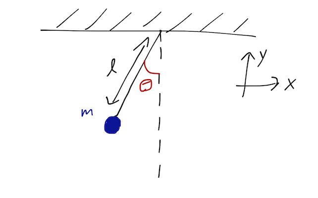
Starting in Cartesian coordinates, we know how to write down the kinetic and potential energies: \mathcal{L} = T - U = \frac{1}{2}m\dot{x}^2 + \frac{1}{2} m\dot{y}^2 - mgy. This is the same Lagrangian as a particle in free-fall; what we’re missing is the fact that this is a pendulum, and the bob is attached to a rod. This gives a constraint on the motion - at any instant, the particle has to be distance \ell from where the rod is attached, x^2 + y^2 = \ell^2. This constraint lets us eliminate one of the two variables; if we specify either x or y, we know immediately the other coordinate. Of course, x and y aren’t the only quantities we can use to describe the pendulum; we know that we usually prefer to work with the angle \theta that the pendulum makes with the vertical. So let’s change coordinates like this: x = \ell \sin \theta \\ y = \ell (1 - \cos \theta) so the derivatives are \dot{x} = \ell \dot{\theta} \cos \theta \\ \dot{y} = \ell \dot{\theta} \sin \theta and the Lagrangian becomes: \mathcal{L} = \frac{1}{2} m \ell^2 \dot{\theta}^2 - mg\ell (1 - \cos \theta). Notice that the kinetic energy looks very familiar: it’s exactly the rotational kinetic energy of the bob, \frac{1}{2} I \omega^2, or \frac{1}{2} mv^2 with v pointing in the tangential \hat{\theta} direction.
Now here’s the fun part. I’m just going to forget that I changed coordinates, and try to write down the Euler-Lagrange equation for the variable \theta. What I find is: \frac{\partial L}{\partial \theta} = -mg\ell \sin \theta \\ \frac{\partial L}{\partial \dot{\theta}} = m \ell^2 \dot{\theta} \\ \frac{\partial L}{\partial \theta} - \frac{d}{dt} \left(\frac{\partial L}{\partial \dot{\theta}}\right) = 0 = -mg\ell \sin \theta - m\ell^2 \ddot{\theta} or dividing through, \ddot{\theta} + \frac{g}{\ell} \sin \theta = 0. This is the correct equation of motion for a pendulum derived using Newton’s laws! We didn’t have to treat \theta any differently just because it was an angle; all we had to do was carry out a single change of coordinates. Fundamentally, this works because Hamilton’s principle and the Euler-Lagrange equations don’t care what our variables are, just that we can write the action in the standard form. In other words, we’ve changed coordinates but not changed the action: S = \int_{t_i}^{t_f} dt\ \mathcal{L}(t, x, \dot{x}, y, \dot{y}) = \int_{t_i}^{t_f} dt\ \mathcal{L}(t, \theta, \dot{\theta}). The variable \theta here is an example of a generalized coordinate (or “GC”), which in general we will denote with the symbol q_i. Generalized coordinates don’t have to have units of length, or even the same units as each other. They just have to be some function of the original Cartesian coordinates and time. If we have N particles in our system, we can write q_i = q_i(\vec{r}_1, \vec{r}_2, \vec{r}_3, ..., \vec{r}_N, t). It’s important that the set of GCs that we choose allow us to uniquely specify the configuration of our physical system. In other words, the equations above have to be invertible so that we can also write \vec{r}_i = \vec{r}_i(q_1, q_2, q_3, ..., q_{dN}, t) Here little d stands for dimension; by default d=3 of course, but we’ll commonly deal with problems (like the pendulum) where we study a two-dimensional system that’s easy to draw on the board. (In the pendulum example above, the z coordinate is ignorable, remember.)
Now we’re starting to see some of the advantages of the Lagrangian approach emerge. The real power of the Lagrangian comes from the fact that it only deals in scalars. To see why this is a big deal, think about what happens when we change from one coordinate system to another:
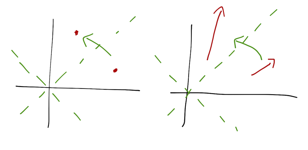
A scalar quantity is just like a point; its position as measured in the new coordinates moves, but that’s it. All we need to know is the functional relationship between the new coordinates and the old: f(x',y',z') = f(x(x',y',z'),y(x',y',z'),z(x',y',z')). On the other hand, vectors have a length and a direction, both of which can change as we shift coordinate systems. We need not just the functional relationship between the coordinates, but also how the unit vectors themselves are changed. If we want to evaluate a gradient or a curl, we have to memorize complicated formulas which take this stretching and twisting of the vectors into account properly.
If we have multiple particles in our system, the simplicity of the Lagrangian approach is compounded further. Suppose we have three electric charges moving around in three dimensions; there are two force vectors on each particle, for a total of 18 independent components of the force to keep track of. But there is only one Lagrangian for the entire system!
8.7 Counting degrees of freedom
How many generalized coordinates do we actually need? This quantity actually has a special name: the number of degrees of freedom of a physical system is the number of GCs required to uniquely describe it. For particles moving freely in space, we see that there are 3N degrees of freedom; each particle has a triplet of coordinates (x,y,z) that we need to specify. But as we saw last time, very often we’re interested in constrained systems. Our concrete example was the simple pendulum in the x-y plane:
The bob can move in 2 directions, but the presence of the string provides the constraint x^2 + y^2 = \ell^2, which means that we can eliminate one variable; the single generalized coordinate \theta is enough to give us both x and y for the bob. In general, counting degrees of freedom is easy:
For a system of N particles in d dimensions, subject to m constraints, the number of degrees of freedom is n_{\rm dof} = dN - m, and n_{\rm dof} generalized coordinates are needed to describe the system.
Let’s run through a few examples! The single pendulum above has d=2, N=1, and m=1, so we find only one degree of freedom - consistent with the one coordinate (\theta) needed to describe the system. The double pendulum is slightly more involved:
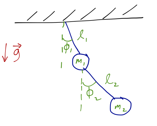
Now clearly N=2, and we identify two constraints (two strings) - so n_{\rm dof} = 4-2 = 2 (hence, two angles will work as a complete set of GCs.) This is easy to extrapolate; the n-tuple pendulum has n degrees of freedom, which are the n angles that each bob makes with the one above it.
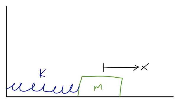
How about something a little different? Consider a block on a frictionless ramp, which is itself free to slide on a frictionless surface:
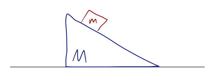
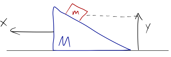
Again N=2 and d=2. We also have 2 constraints again; the block stays on the ramp, and the ramp stays on the surface. So we expect to need two coordinates. One possibility is the x-position of the ramp, and the height of the block:
But an equally valid choice for the second coordinate would be the distance the block has traveled down the ramp:
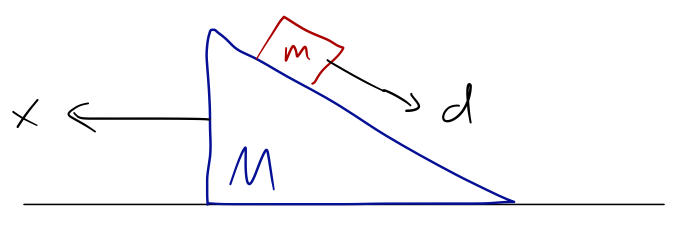
This second choice of coordinates probably looks a bit weird to you, and it’s a good example of two key facts about generalized coordinates. First, in general the choice of GCs is not unique for any given problem! Of course, many problems will be significantly easier to solve with the right choice of coordinates; it will take some practice and intuition to be able to make such a choice consistently.
Second, this illustrates the key difference between generalized coordinates and the more ordinary coordinate systems that you’re familiar with, e.g. spherical or cylindrical coordinates. All of the standard coordinate systems you know are orthogonal coordinate systems - which means that the unit vectors are perpendicular to one another. Here, x and d are (clearly) not orthogonal!
Doing anything with vectors in a basis which isn’t orthogonal is, as you can imagine, a horrible experience. But again, now that we’re using the Lagrangian approach we don’t care about vectors, which means we don’t care about orthogonality (or even about unit vectors.)
There is one important caveat, which is that only certain types of constraints are allowed in the Lagrangian formalism as we’re using it (without violating assumptions we’ve made or leading to a bad change of coordinates.) Specifically, we can apply any constraint that can be written in the form f_\alpha(\vec{r}_1, \vec{r}_2, ..., \vec{r}_N, t) = 0. This is called a holonomic constraint. This is a somewhat formal way of writing it out: the key features of a holonomic constraint are
- It’s an equation, not an inequality;
- It depends only on positions and time, not on velocities;
- It doesn’t depend on any information other than the coordinates of the objects (and time.)
A physical system with only holonomic constraints is said to be holonomic; we can only apply our Lagrangian formalism to holonomic systems.
8.8 More Lagrangian examples
The best way to recognize a holonomic constraint is actually just to recognize cases that aren’t holonomic. The two most common non-holonomic constraints to watch out for are inequalities, or systems where the final state depends not just on the coordinates but on the path taken.
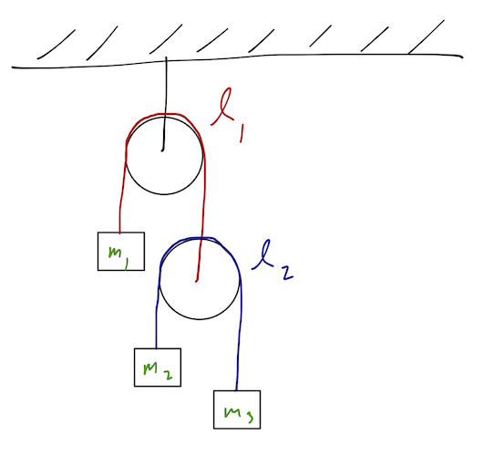
8.8.1 Example: double Atwood’s machine
Also known as the “double pulley” system; the setup is as drawn below. The constraints are clearly holonomic, given by the strings over the (massless) pulleys. We assume, as is usual for a pulley problem, that the blocks only move up and down, and don’t swing from side to side.
Let me draw out all of the positions of the blocks using the generalized coordinates we chose:
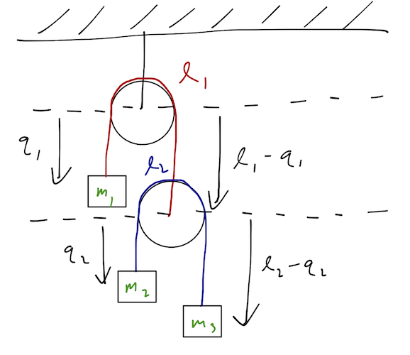
Here I am assuming the radius of the pulleys is negligible, i.e. the length of the rope which loops around the top of the pulley is much smaller than the total length \ell. (Nothing interesting would change without this assumption, we’d just get an extra constant in the coordinates on the right-hand side of the diagram.)
Now, let’s compute the Lagrangian. The kinetic energy is easy enough to calculate, but we have to make sure to start in the inertial frame! Let’s be very careful and start with a Cartesian coordinate system: we’ll take y to point up with origin at the center of the top pulley. Then the y-coordinates of the three masses are: y_1 = -q_1 \\ y_2 = -\ell_1 + q_1 - q_2 \\ y_3 = -\ell_1 - \ell_2 + q_1 + q_2 We always know how to write the kinetic energy in Cartesian coordinates: T = \frac{1}{2} m_1 \dot{y}_1^2 + \frac{1}{2} m_2 \dot{y}_2^2 + \frac{1}{2} m_3 \dot{y}_3^2. Taking time derivatives above and substituting in, we arrive back at the answer we found last time: T = \frac{1}{2} m_1 \dot{q}_1^2 + \frac{1}{2} m_2 (\dot{q}_1 - \dot{q}_2)^2 + \frac{1}{2} m_3 (\dot{q}_1 + \dot{q}_2)^2 \\ = \frac{1}{2} (m_1 + m_2 + m_3) \dot{q}_1^2 + \frac{1}{2} (m_2 + m_3) \dot{q}_2^2 + (m_3 - m_2) \dot{q}_1 \dot{q}_2.
This is more complicated than you might have guessed T would look! In particular, the kinetic energy of the blocks is not just T \neq \frac{1}{2} m_1 \dot{q}_1^2 + \frac{1}{2} (m_2 + m_3) \dot{q}_2^2. which you might guess if you went too quickly from the diagram. If you think carefully, our result for T does make sense: it’s fairly obvious that the speed of, say, block m_2 will depend on both q_1 and q_2, and so we can just write down the speeds and compute everything as T = \frac{1}{2} mv^2, and we’ll be fine. But the conversion isn’t so obvious for every set of GCs you’ll run into. When in doubt, always start in a Cartesian coordinate system and convert to generalized coordinates!
Now we’re ready to move on to the potential energy. Again, it’s easiest to start in our Cartesian coordinates where we know the answer: U = m_1 g y_1 + m_2 g y_2 + m_3 g y_3 \\ = -m_1 g q_1 - m_2 g(\ell_1 - q_1 + q_2) - m_3 g (\ell_1 + \ell_2 - q_1 - q_2) \\ = -(m_1 - m_2 - m_3)g q_1 - (m_2 - m_3)g q_2 where I’ve dropped all of the constant terms from U, which we’re of course free to do by re-zeroing the potential. (Whatever constants are there won’t appear in the Euler-Lagrange equations anyway.) Combining into \mathcal{L} = T - U, the Euler-Lagrange equations are: \frac{\partial \mathcal{L}}{\partial q_i} - \frac{d}{dt} \left(\frac{\partial \mathcal{L}}{\partial \dot{q_i}}\right) = 0 or, expanding out from above, (m_1 - m_2 - m_3) g = (m_1 + m_2 + m_3) \ddot{q_1} + (m_3 - m_2) \ddot{q_2} \\ (m_2 - m_3) g = (m_2 + m_3) \ddot{q_2} + (m_3 - m_2) \ddot{q_1}. This motion is, as we might expect, pretty simple; we just have two accelerations and a bunch of constants. We could go on to solve for the full motion in terms of q_1 and q_2 just by rearranging things and integrating twice, but I’ll stop here - the algebra is too tedious for the blackboard. As a cross-check, we can already notice that the equilibrium points indicated by this solution make physical sense: if m_2 = m_3, then the second equation gives \ddot{q_2} = 0, which makes sense because the lower pulley is balanced. For the upper pulley, from the first equation if we have m_1 = m_2 + m_3 and m_2 = m_3, then the system is balanced and again there is no acceleration (\ddot{q_1} = \ddot{q_2} = 0.)