15 Hamiltonian mechanics and phase space
15.1 Phase space
In exploring the behavior of the Lotka-Volterra equations, we relied heavily on numerical study of how solutions evolve in the plane of the two variables R and F, hiding the dependence on the independent variable t. The space of R and F is known as the state space, and we can make powerful observations such as the fact that no two paths will cross.
Can we apply these geometric ideas to a physical system that has non-linear dynamics, like, say, the simple pendulum? \ddot{\theta} = -\frac{g}{L} \sin \theta. Our first problem is that this is now a second-order differential equation; we could try to plot \ddot{\theta} vs. \theta, but that doesn’t give us enough information to tell how the system evolves, since it depends on \dot{\theta} at that instant too.
Now what? Let’s refresh our memory about exactly where the equation of motion comes from. At the beginning of the semester, we introduced Lagrangian mechanics as a radical new way of looking at (and solving for the motion of) mechanical systems.
One of the central concepts that we introduced was the idea of a generalized coordinate, q_i. The q_i are a set of functions of the spatial coordinates of all of the objects in our system, plus time: q_i = q_i(\vec{r}_1, \vec{r}_2, ..., \vec{r}_N, t). With three spatial dimensions, and with m constraints on the system, we need 3N - m independent generalized coordinates to describe the position of the system.
With the Lagrangian and the generalized coordinates in hand, the motion of the system is described by the Euler-Lagrange equations, \frac{\partial \mathcal{L}}{\partial q_i} = \frac{d}{dt} \left( \frac{\partial \mathcal{L}}{\partial \dot{q_i}} \right). At the very end of our discussion of Lagrangian mechanics, we came to the idea of conserved quantities, that is to say, quantities which don’t change as the system evolves (total energy E is the most familiar example you know.) From studying the Euler-Lagrange equations, we found in particular that if the Lagrangian is independent of any of the q_i, so \partial \mathcal{L} / \partial q_i = 0, then \frac{\partial \mathcal{L}}{\partial q_i} = 0 \Rightarrow \frac{\partial \mathcal{L}}{\partial \dot{q}_i} \equiv p_i = \textrm{const}. The p_i is the generalized momentum associated with coordinate q_i; for a Cartesian coordinate like x, it’s just the linear momentum p_x.
Now, notice that even if \partial \mathcal{L} / \partial q_i \neq 0, we can still write the equation of motion in terms of the momentum, except now it’s not constant anymore: \frac{\partial \mathcal{L}}{\partial q_i} = \dot{p_i}. This is a first-order differential equation for the momentum, p_i! Let’s go back to the pendulum example: the Lagrangian for the simple pendulum is \mathcal{L} = \frac{1}{2} m L^2 \dot{\theta}^2 + mgL \cos \theta so the generalized momentum is p_\theta = mL^2 \dot{\theta}, and its differential equation is \dot{p}_\theta = -mgL \sin \theta. We have reduced one second-order differential equation to a pair of first-order equations (in general, N second-order diff eqs give us 2N first-order ones.) The space defined by the combination of generalized coordinates q_i and their associated generalized momenta p_i is known as phase space.
Now we can plot the gradient in the space of (\theta, p_\theta), just as we did for the Lotka-Volterra equations! Let’s set m = L = g = 1 and just focus on the numerics.
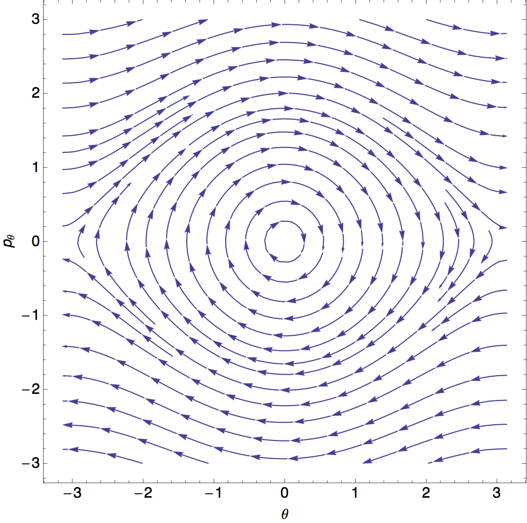
This is a (graphical) solution to the pendulum, for arbitrary angles, no small-angle approximation needed! (Such a sketch in phase space is known as a phase portrait.) For small angles, we see circles corresponding to simple harmonic motion: if our small-angle solution is \theta(t) \propto \cos(t), then p_\theta \propto \dot{\theta} \propto \sin(t), which is the parametric equation for a circle.
At large p_\theta, meanwhile, we can also easily visualize the motion: up to small fluctuations, p_\theta remains large and roughly constant through the motion. This corresponds to the pendulum swinging in a circle around the support (remember that \theta = -\pi and \theta = +\pi are the same point, so every curve here is still closed!)
There is a single curve separating back-and-forth harmonic motion from the constant spinning motion; it’s called the separatrix, and it’s the phase-space path that is still a closed loop, but just barely touches \theta = -\pi and \theta = \pi. The motion of the pendulum along the separatrix is particularly funny; it comes to a (nearly) complete stop in a (nearly) vertical position, then falls back down the other way, and repeats. (Of course, if we have exactly \theta = \pi and p_\theta = 0, the pendulum doesn’t move at all. This is an unstable equilibrium point.)
This is a lot of progress for one small plot! Using phase space to split our equations of motion into coupled first-order differential equations is a very powerful technique. However, things were particularly simple here, especially the equation p_\theta = \partial \mathcal{L} / \partial \theta. In general, just using that equation won’t just lead us to a simple first-order differential equation; the derivative could be some more complicated function of the coordinate derivatives.
But don’t give up yet, because there is a way to generally arrive at first-order equations, and that is through the Hamiltonian.
15.2 Hamiltonian mechanics
Way back in our study of Lagrangian mechanics, we defined an object called the Hamiltonian, \mathcal{H} = \sum_i p_i \dot{q}_i - \mathcal{L}, where q_i are generalized coordinates and p_i are their associated generalized momenta, p_i = \frac{\partial \mathcal{L}}{\partial \dot{q}_i}. We observed at the time that with certain assumptions (no time-dependent coordinates), the Hamiltonian was equal to the total energy - and in any case, it is always a conserved quantity, d\mathcal{H} / dt = 0, as a consequence of time translation invariance.
Now we’re ready to see an application of the Hamiltonian, which is working in phase space. Let’s focus for the moment on the case of a single q; generalizing to many coordinates is easy. Then I can drop the sum, and just write \mathcal{H} = p\dot{q} - \mathcal{L}. Since we want to work in phase space, we should treat \dot{q} as a function of the phase-space variables: \dot{q} = \dot{q}(q,p). (Remember, we have an equation defining p from the derivative \partial \mathcal{L} / \partial q; we can just go back and invert it to get this function, usually.) With this replacement, the full Hamiltonian (and the Lagrangian) can be written as functions of only p and q: \mathcal{H}(p,q) = p \dot{q}(p,q) - \mathcal{L}(q, \dot{q}(p,q)). Now let’s start taking derivatives, and see if applying the Euler-Lagrange equations of motion will get us anywhere. First, \frac{\partial \mathcal{H}}{\partial q} = p \frac{\partial \dot{q}}{\partial q} - \left[ \frac{\partial \mathcal{L}}{\partial q} + \frac{\partial \mathcal{L}}{\partial \dot{q}} \frac{\partial \dot{q}}{\partial q} \right] (this is a straightforward application of the chain rule.) But we know already that by definition, \partial \mathcal{L} / \partial \dot{q} = p. So two of the terms cancel, and we just have \frac{\partial \mathcal{H}}{\partial q} = - \frac{\partial \mathcal{L}}{\partial q} Now, we remember the Euler-Lagrange equation: the right-hand side is the time derivative of \partial \mathcal{L} / \partial \dot{q}, which we recognize once again is just p. Thus, \frac{\partial \mathcal{H}}{\partial q} = -\dot{p}. The other variable we have lying around is p: \frac{\partial \mathcal{H}}{\partial p} = \dot{q} + p \frac{\partial \dot{q}}{\partial p} - \frac{\partial \mathcal{L}}{\partial \dot{q}} \frac{\partial \dot{q}}{\partial p}. This time the last two terms cancel, and so we have \frac{\partial \mathcal{H}}{\partial p} = \dot{q}. This is exactly what we were looking for — a set of coupled, but first-order differential equations of motion!
If the derivation feels arbitrary or miraculous: there is a general mathematical technique called the Legendre transformation which allows second-order differential equations to be traded for first-order ones by introducing an auxiliary variable like the momentum here. If you’ve taken a math class in diff-eq, you may have seen the Legendre transform before.
As I said, the derivation for a larger number of coordinates isn’t very difficult. If you do it, you will arrive at Hamilton’s equations.
\dot{p}_i = -\frac{\partial \mathcal{H}}{\partial q_i}, \qquad \dot{q}_i = \frac{\partial \mathcal{H}}{\partial p_i}. If \partial \mathcal{H} / \partial q_i = 0, then the corresponding momentum p_i is conserved: \dot{p}_i = 0.
While we’re thinking about time-dependence, we recall that in many situations \mathcal{H} = T + U, but only when the coordinates are all independent of time, i.e. \partial q_i / \partial t = 0. (Note that this includes coordinates that are eliminated by constraints, if the constraint is time-dependent; you should be careful with such situations.) It’s straightforward to show the relations: \frac{d\mathcal{H}}{dt} = \frac{\partial \mathcal{H}}{\partial t} = -\frac{\partial \mathcal{L}}{\partial t}. which is another way of stating that if the Hamiltonian has no explicit time dependence, i.e. \partial \mathcal{H} / \partial t = 0, then it is totally conserved, d\mathcal{H} / dt = 0.
For the pendulum, we made a big deal out of the fact that paths in phase space can’t cross, because given all the p_i and q_i, the derivatives give us a unique direction in phase space in which the system will evolve in an infinitesimal time dt. Note that this is only true if \partial \mathcal{H} / \partial t = 0; if \mathcal{H} is changing, then knowing just p_i and q_i isn’t sufficient to tell us the derivatives. (Hamilton’s equations will work just fine whether there’s extra time-dependence or not, but making sketches in phase space is much less useful.)
Going beyond the simplest problems, we won’t be able to simply draw phase-space diagrams on the board; even for just two independent non-ignorable coordinates, the phase space becomes 4-dimensional (good luck drawing that.) But we can still use the language of geometry in this higher-dimensional space to make some progress. In general, we can combine the coordinates q_i and momenta p_i into one large 2N-component phase-space vector: \vec{z} = (\vec{q}, \vec{p}) = (q_1, ..., q_n, p_1, ..., p_n). This is sometimes also known as the phase point. Thanks to the Hamiltonian approach, we can write down Hamilton’s equations, which give us a single vector-valued differential equation: \dot{\vec{z}} = \vec{h}(\vec{z}). I’ve written the function \vec{h} itself as a vector, to remind us that this isn’t just a function of a vector, it’s 2n independent functions coming from Hamilton’s equations. (If all of the functions \vec{h} are linear then we can write it as a matrix, but that’s not guaranteed.)
Note also that if \partial \mathcal{H} / \partial t \neq 0, then we actually have \dot{\vec{z}} = \vec{h}(\vec{z}, t); this will complicate some of the discussion we’re about to have, so I’ll assume time-independence for now. Combining p and q into a large vector is made possible by the fact that in the Hamiltonian approach, we treat positions and momenta on (nearly) equal footing. This equal treatment enables some other interesting tricks, which I won’t go into here (but you’ll find such devices as canonical transformations if you go on to study graduate-level classical mechanics.)
15.3 Solving with Hamilton’s equations
Although the main motivation we had for coming this far was to think in terms of phase space (which will have some further nice, geometric properties which we will come to!), Hamilton’s equations also provide us with yet another way to find the motion of a dynamical system.
- Set up the Lagrangian as usual, with some generalized coordinates q_i.
- Find the generalized momenta p_i = \partial \mathcal{L} / \partial \dot{q}_i.
- Solve for \dot{q}_i in terms of the p_i and q_i.
- Rewrite T and U in terms of q_i and p_i.
- Find \mathcal{H}, as T+U if all the \partial q_i/\partial t = 0 (including constraints!), otherwise as \sum_i p_i \dot{q}_i - \mathcal{L}.
- Apply Hamilton’s equations to get the equations of motion: \dot{p}_i = -\frac{\partial \mathcal{H}}{\partial q_i}, \qquad \dot{q}_i = \frac{\partial \mathcal{H}}{\partial p_i}.
Once we have the equations of motion, we can look for equilibrium points, make phase-space portraits, solve for q_i(t) explicitly, etc.
A very common mistake when trying to use Hamilton’s equations is putting the minus sign in the wrong place. A quick and easy way to remember is to apply it to the free Hamiltonian: for a single particle in one dimension with U = 0, we have \mathcal{H}_{\rm free} = T = p^2 / (2m). Then the second of Hamilton’s equations gives \dot{q} = p/m, which is just the usual definition of linear momentum — with no minus sign.
We need one simple example here to get a better feeling for how Hamiltonian mechanics works in practice.
15.3.1 Example: the simple harmonic oscillator
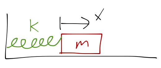
We’ll take x as our lone generalized coordinate. We all know how to write this Lagrangian in our sleep: \mathcal{L} = \frac{1}{2} m \dot{x}^2 - \frac{1}{2} kx^2. The generalized momentum is just the linear momentum, but let’s do it the careful way: p_x = \frac{\partial \mathcal{L}}{\partial \dot{x}} = m \dot{x}, so \dot{x} = p_x / m.
Let’s find the Hamiltonian the careful way first. Rewriting the Lagrangian, we have: \mathcal{L} = \frac{p_x^2}{2m} - \frac{1}{2} kx^2. Applying the general formula for the Hamiltonian gives \mathcal{H} = p_x \dot{x} - \mathcal{L} \\ = p_x \dot{x} - \frac{p_x^2}{2m} + \frac{1}{2} kx^2 \\ = \frac{p_x^2}{2m} + \frac{1}{2} kx^2 which is of course just T + U, since in this case we have no time-dependent coordinates or constraints.
Now we can take derivatives to get Hamilton’s equations: \dot{p_x} = -\frac{\partial \mathcal{H}}{\partial x} = -kx \\ \dot{x} = \frac{\partial \mathcal{H}}{\partial p_x} = \frac{p_x}{m}. Ironically enough, the easiest way to solve this is just to plug one equation into the other, say by taking the derivative of the \dot{x} equation: \ddot{x} = \frac{\dot{p_x}}{m} = -\frac{k}{m} x which should look very familiar by now. We could draw the phase-space plot, but it will be unsurprisingly boring: we know the solution is just a simple harmonic oscillator no matter what x or p_x are. Explicitly, the gradient of (x, p_x) is (\dot{x}, \dot{p}_x) = (p_x/m, -kx) We can use this numerically, but since we’re drawing paths that the system follows through time, we can also use the solution that we already know: x = x_0 \cos(\sqrt{k/m} t - \delta) \\ p_x = m\dot{x} = -mx_0 \sqrt{k/m} \sin (\sqrt{k/m} t - \delta) This is just the equation for a ellipse, with the polar angle given by the argument of the cosine. We can see this explicitly by noticing that \frac{x^2}{x_0^2} + \frac{p_x^2}{mkx_0^2} = \cos^2 (...) + \sin^2 (...) = 1 which is the standard equation for an ellipse in the x-p_x plane; the axes are 2x_0 and 2\sqrt{mk} x_0.
15.4 Liouville’s theorem
We’ve focused a lot on individual phase-space trajectories, where we pick some exact starting value for our mechanical system and then just let it evolve. But in the real world, we can never be exactly certain of the state of our system; there will always be some measurement error. Because of this, it’s an interesting question to ask not just how a point evolves in phase space, but how a volume will evolve. If we only know that our system’s initial state lies within some volume, how accurately can we predict where it will be in the future?
(Incidentally, the idea of phase space volumes is also very useful if we’re studying a large collection of particles, like a gas, something which really would occupy a volume in phase space even if we didn’t have any measurement uncertainty.)
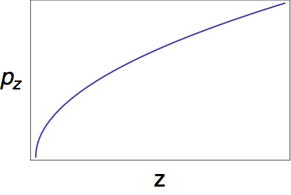
Let’s consider a simple example, that of a particle in freefall, just to see what happens. What is the phase-space trajectory of a single particle in freefall? We know that \dot{p_z} = mg and \dot{z} = -gt. But we want to plot in terms of z = \frac{1}{2} gt^2 and p_z = mgt. So, we see that z \propto p_z^2, which is the equation for a sideways parabola (or a square-root function):
If we change the initial conditions, then the trajectory will start at a different point, but will still be described by a sideways parabola. If we start with an initial region, say a square, its area will be distorted as the points within it evolve in time:
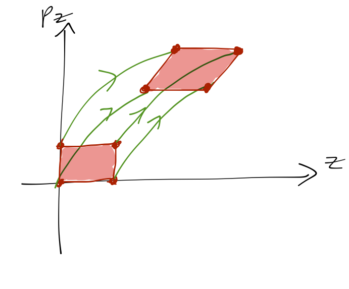
(A region like this might represent some uncertainty in setting or measuring our initial conditions, for example.) Although our initial region of phase space has become distorted by the time evolution of the system, the area of the region is the same before and after — a very powerful and general result of Hamiltonian mechanics.
If we start with a phase-space volume and let it evolve according to some Hamiltonian, the volume of that region does not change, no matter how its shape is distorted.
Taylor has a derivation of Liouville’s theorem involving vector calculus, but it’s a somewhat long and involved argument, so I’m going to show you another way to derive it. Once again I’ll do the derivation with a single coordinate and single momentum (q,p); it’s very easy to generalize. Suppose we have a really tiny volume of phase space centered around the point \vec{z}_0 = (q_0, p_0). V = dq dp. Now we let our tiny volume evolve for an infinitesimal time step, dt. We know that the center point \vec{z}_0 evolves according to Hamilton’s equations, i.e. q_0 \rightarrow q_0 + \dot{q} dt = q_0 + \frac{\partial \mathcal{H}}{\partial p} dt = \tilde{q}_0,\\ p_0 \rightarrow p_0 + \dot{p} dt = p_0 - \frac{\partial \mathcal{H}}{\partial q} dt = \tilde{p}_0. The small volume evolves in the same way: \tilde{V} = d\tilde{q} d\tilde{p} = (\det J) V where J is the Jacobian matrix describing the change of coordinates. This factor is completely familiar as the extra term which appears when we do integrals in spherical or cylindrical coordinates. In general, the Jacobian is a matrix of all the partial derivatives given by our coordinate change: in index notation, J_{ij} = \frac{\partial \tilde{z}_i}{\partial z_j} or explicitly in this case, \mathbf{J} = \left( \begin{array}{cc} \partial \tilde{q} / \partial q & \partial \tilde{q} / \partial p \\ \partial \tilde{p} / \partial q & \partial \tilde{p} / \partial p \end{array} \right) \\ = \left( \begin{array}{cc} 1 + (\partial^2 \mathcal{H} / \partial p \partial q) dt & (\partial^2 \mathcal{H} / \partial p^2) dt \\ - (\partial^2 \mathcal{H} / \partial q^2) dt & 1 - (\partial^2 \mathcal{H} / \partial q \partial p) dt \end{array} \right). and the determinant is \det J = 1 - (\partial^2 \mathcal{H} / \partial p \partial q)^2 dt^2 + (\partial^2 \mathcal{H} / \partial p^2) (\partial^2 \mathcal{H} / \partial q^2) dt^2 \\ = 1 + (...) dt^2 + ... The key point here is that there is no linear term in dt, which means that \frac{d (\det J)}{dt} = 0 \Rightarrow \tilde{V} = V. (This is sort of trivial here, but if we had more than one variable q, then the vanishing of the linear term involves canceling the partial derivatives on the diagonal against each other.) This is Liouville’s theorem.
This is a little reminiscent of Heisenberg’s uncertainty principle, in fact; if we start with some distribution of particles with spread \Delta q and \Delta p in their positions and momenta, then Liouville’s theorem tells us that the product \Delta q \Delta p is constant as the system evolves. If we try to squeeze the particles together, their momenta will spread apart, and vice-versa. (The uncertainty principle is much deeper, the main difference being that there is no lower bound on the initial product \Delta q \Delta p in classical mechanics.)
15.5 Worked examples
15.5.1 Example: mass on a cone
Let’s do another example which is a little more elaborate, and which shows off some of the advantages of the Hamiltonian approach. Consider a mass m which moves without friction on the surface of a cone, with opening angle \alpha, and subject to gravity in the -z direction:
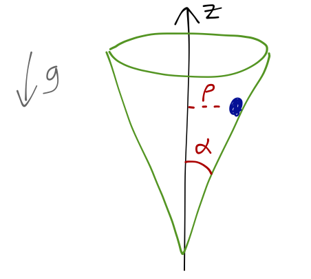
Let’s start by finding the Lagrangian. Clearly, cylindrical coordinates are the way to go here; the Lagrangian is then \mathcal{L} = \frac{1}{2} m (\dot{\rho}^2 + \dot{z}^2 + \rho^2 \dot{\theta}^2) - mgz. Since our particle is stuck to the surface of the cone, we have a constraint between z and \rho, \rho = z \tan \alpha. Plugging back in to eliminate z, we have (since \dot{z} = \dot{\rho} \cot \alpha) \mathcal{L} = \frac{1}{2} m (\dot{\rho}^2 (1 + \cot^2 \alpha) + \rho^2 \dot{\theta}^2) - mg \rho \cot \alpha. Now, we take derivatives to find the two generalized momenta: p_\theta = \frac{\partial \mathcal{L}}{\partial \dot{\theta}} = m\rho^2 \dot{\theta} \\ p_\rho = \frac{\partial \mathcal{L}}{\partial \dot{\rho}} = m \dot{\rho} (1 + \cot^2 \alpha). These are nice and easy to solve for \dot{\rho} and \dot{\theta}; we just divide through by the constant stuff. Moreover, our generalized coordinates are independent of time, so we know we can write \mathcal{H} = T + U. So, taking these and plugging back in to the kinetic energy T, we have \mathcal{H} = \frac{1}{2} m \left(\frac{p_\rho}{m (1+\cot^2\alpha)}\right)^2 (1 + \cot^2 \alpha) \\ + \frac{1}{2} m \rho^2 \left(\frac{p_\theta}{m\rho^2}\right)^2 + mg \rho \cot \alpha \\ = \frac{p_\rho^2}{2m (1 + \cot^2 \alpha)} + \frac{p_\theta^2}{2m\rho^2} + mg \rho \cot \alpha. Hamilton’s equations for \theta are pretty simple: \dot{p}_\theta = -\frac{\partial \mathcal{H}}{\partial \theta} = 0 \\ \dot{\theta} = \frac{\partial \mathcal{H}}{\partial p_\theta} = \frac{p_\theta}{m\rho^2}. So the second equation gave us back the definition of p_\theta, and the first told us that p_\theta is constant. Because \dot{p}_{\theta} = 0, we say that \theta is an ignorable coordinate. Note that this does not mean that \theta is a constant, too; in fact, we can see that \dot{\theta} is generally non-zero and can even change, as long as \rho evolves in time.
Given these complications, what does “ignorable” even mean? We know two things about \theta: that \partial \mathcal{H} / \partial \theta = 0, and that p_\theta is a constant. But this means that the Hamiltonian itself can be written as \mathcal{H} = \mathcal{H}(\rho, p_\rho, p_\theta) and p_\theta is a constant; in other words, the Hamiltonian is now a function only of two variables, not four! Explicitly, if we write out the other two equations for \rho, we find \dot{p}_\rho = -\frac{\partial \mathcal{H}}{\partial \rho} = \frac{p_\theta^2}{m\rho^3} - mg \cot \alpha \\ \dot{\rho} = \frac{\partial \mathcal{H}}{\partial p_\rho} = \frac{p_\rho}{m (1 + \cot^2 \alpha)}. This describes an equivalent one-dimensional problem, because the only variables in these equations that are time-dependent are \rho and p_\rho; we could combine them into a single second-order differential equation for \rho. Taking the derivative of the second equation, \ddot{\rho} = \frac{1}{m(1+\cot^2 \alpha)} \dot{p}_\rho = \frac{1}{m(1+\cot^2 \alpha)} \left( \frac{p_\theta^2}{m\rho^3} - mg \cot \alpha \right). This is a hard equation to solve directly. But there’s another trick up our sleeve; we can notice that the Hamiltonian can be rewritten in the form \mathcal{H}_{1d} = \frac{p_\rho^2}{2\mu} + U_{\textrm{eff}}(\rho) where \mu = m (1 + \cot^2 \alpha) = m/\sin^2 \alpha \\ U_{\textrm{eff}} = \frac{p_\theta^2}{2m\rho^2} + mg\rho \cot \alpha. We have done this trick before, of course, when we first solved the central-force motion problem. But notice that it is much easier in the Hamiltonian approach. All we have to do is look at \mathcal{H}, notice that p_\theta is conserved since there’s no \theta dependence, and just read off the equivalent one-dimensional problem for \rho. If instead we tried to use the Lagrangian, we would have to be careful when taking the equations of motion and trying to plug back in to find the equivalent problem, because there are crucial minus signs lurking!
The Hamiltonian approach also easily generalizes to many ignorable coordinates: we just identify them (by noticing that \partial \mathcal{H} / \partial q_i = 0), and then immediately focus on solving for the remaining non-ignorable coordinates.
(This arises from the fact that our assumption in deriving the Lagrangian equations of motion was that \dot{\theta} was held fixed at the endpoints of the path; but as we’ve seen, this isn’t the same as p_\theta staying fixed. The Hamiltonian approach, on the other hand, treats momentum and coordinate as separate variables, so we don’t have to worry about this subtlety.)
To finish our solution, notice that we can draw the effective potential for \alpha > 0 and p_\theta > 0, and it looks like this:
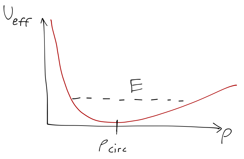
Clearly, any orbit within the cone is bound; at the minimum of the potential, we find the usual circular orbit: \frac{dU_{\textrm{eff}}}{d\rho} = -\frac{p_\theta^2}{m\rho^3} + mg \cot \alpha = 0 \\ \Rightarrow \rho_{\textrm{circ}} = \left( \frac{p_\theta^2 \tan \alpha}{m^2 g} \right)^{1/3}. We could also try to make a phase-space plot of \rho and p_\rho, but we already know from the effective potential analysis that it won’t be very interesting; for any initial point (\rho, p_\rho) we’ll just find periodic motion between the minimum and maximum \rho values given by setting E = U_{\textrm{eff}}(\rho).
15.5.2 Example: a springy Atwood’s machine
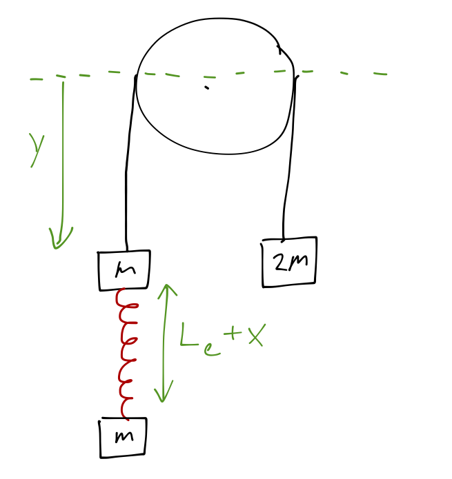
The setup is as drawn in the sketch. The gravitational potential isn’t too hard to write down: U_g = (2m)gy - mgy - mg(x+y) = -mgx. We’re given the equilibrium length L_e of the spring to work with; at equilibrium the spring and gravitational forces balance, i.e. k(L_e - L_0) = mg where L_0 is the unstretched length of the spring. The extension of the spring in total is thus (x + L_e) - L_0 = x + \frac{mg}{k}. We can plug back in to find the spring potential, U_k = \frac{1}{2} k \left(x + \frac{mg}{k}\right)^2 \\ = \frac{1}{2} kx^2 + mgx + (\textrm{const}). Despite the rather complicated setup, our total potential energy is extremely simple, and doesn’t even depend on gravity: the mgx terms cancel, and we simply find U = \frac{1}{2} kx^2. For the kinetic energy, we have T = \frac{1}{2} (2m) \dot{y}^2 + \frac{1}{2} m \dot{y}^2 + \frac{1}{2} m (\dot{x} + \dot{y})^2 = \frac{1}{2} m \left[ 3\dot{y}^2 + (\dot{x} + \dot{y})^2\right]. Clearly in this case, the coordinates don’t depend explicitly on time. (The vertical position of the lowest block depends on both x and y, but that’s perfectly fine!) So we can definitely write the Hamiltonian using the shortcut form \mathcal{H} = T + U. The momenta are defined by p_x = \frac{\partial \mathcal{L}}{\partial \dot{x}} = m (\dot{x} + \dot{y}) \\ p_y = \frac{\partial \mathcal{L}}{\partial \dot{y}} = m (4\dot{y} + \dot{x}) which we can invert to get \dot{x} + \dot{y} = \frac{p_x}{m} \\ \dot{y} = \frac{1}{3m} (p_y - p_x). Thus the Hamiltonian turns out to be \mathcal{H} = \frac{1}{2m} \left[ \frac{(p_x - p_y)^2}{3} + p_x^2 \right] + \frac{1}{2}kx^2. Since \partial \mathcal{H} / \partial y = 0, we see that y is ignorable, and thus p_y is a constant. The good news is that this reduces our problem to an equivalent one-dimensional one. The bad news is that we can’t rewrite it using an effective potential, because for p_y \neq 0 there is a term linear in p_x. But as a special case, if we start the apparatus from rest (\dot{x}(0) = \dot{y}(0) = 0), then p_y = 0 and I simply have \mathcal{H} = \frac{2p_x^2}{3m} + \frac{1}{2} kx^2 This is an effective one-dimensional problem for a simple harmonic oscillator, with mass \mu = 3m/4. So we can immediately see that when the system starts from rest, it will undergo simple harmonic motion in x at a frequency \omega^2 = k/\mu = 4k/3m: x(t) = x_0 \cos (\sqrt{4k/3m}t) Once again, don’t forget that y does change even though p_y is zero for all time! I can see this from the fact that \dot{y} depends on both p_y and p_x. If we go back and plug in to Hamilton’s equations we will find that y also oscillates at the same frequency.
What if we actually wanted to solve for x? We haven’t written Hamilton’s equations yet: for p_x, we have \dot{p}_x = -\frac{\partial \mathcal{H}}{\partial x} = -kx \\ \dot{x} = \frac{\partial \mathcal{H}}{\partial p_x} = \frac{4p_x - p_y}{3m} or taking the derivative of the second equation, \ddot{x} = \frac{4\dot{p}_x}{3m} = -\frac{4k}{3m} x. So the result is actually quite simple: even if p_y \neq 0, x still undergoes simple harmonic motion at the same frequency.