16 Continuum mechanics
This chapter is an optional topic. It builds on the coupled-oscillator chapter and provides a bridge to the wave equation and continuum mechanics, but the rest of the book does not depend on it.
16.1 Intro to continuum mechanics
We’ve spent almost all of our time this semester (and in most physics classes) studying the motion of point masses. Point masses are nice objects to deal with mathematically, since we only need up to three coordinates (x,y,z) to specify where they are at a given instant. When we came to rigid bodies, we found that now we needed six coordinates, the three for position and then three Euler angles, to specify both its position and its orientation. (And adding the new coordinates made things much more complicated!)
First, the bad news: there are lots of physical systems for which, in principle, we need many more coordinates. In fact, for anything which is deformable, i.e. something that can change its shape (the opposite of a rigid body) like a pool of water or a rubber ball, we need a near-infinte number of coordinates to describe every possible type of motion it can undergo (even a relatively small object contains a trillion trillion atoms.) Worse, almost every real physical object isn’t rigid under the right circumstances; even something like the Earth’s crust or a ten-story building will flex and deform during an earthquake.
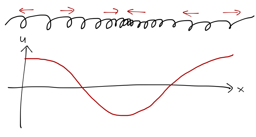
The good news is that it’s actually easier to deal with a nearly-infinite number of degrees of freedom than it would be to deal with a large but finite number! Our starting point will be what Taylor calls the “continuum hypothesis”, but what I would say is more accurately the continuum approximation; namely, that we can assume that a deformable object really is continuous, and ignore the fact that if we zoom in far enough on, say, a string we will eventually find granularity at the level of molecules and atoms. The continuum approximation lets us use continuous functions to describe the configuration of our object. For example, if we consider a string moving in one dimension (up and down), we can write the vertical displacement of the string as a function u(x):
![]()
We’ve actually dealt with continuous objects in a couple of examples before; using the calculus of variations, we were able to find the shape of a soap film or of a string hanging under the influence of gravity. But these are all statements of equilibrium; the subject of continuum mechanics, which we will be studying over the next week, is mainly concerned with the dynamics of continuous objects. Our first step will be to derive the equations which describe continuous motion, by taking the limit of an infinite system from a finite one.
16.1.1 The one-dimensional continuous spring
As a starting point, let’s go back to the one-dimensional system of masses and springs from the coupled oscillator lecture.
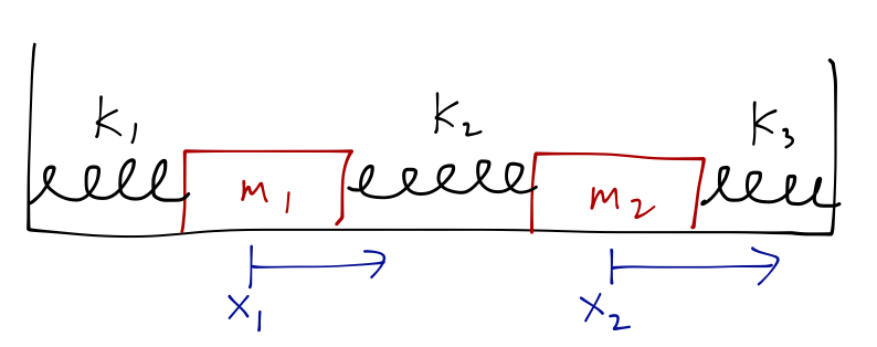
For simplicity, and because continuous objects tend to have uniform properties along their length, we’ll take all the masses and spring constants equal. We could try to use our standard coupled oscillator solution: the matrix \overset{\leftrightarrow}{M} is just m times the identity, and as for \overset{\leftrightarrow}{K}, we saw that for two coupled masses, it took the form
\overset{\leftrightarrow}{K} = \left( \begin{array}{cc} 2k & -k \\ -k & 2k \end{array} \right).
If we go on to the same setup with three masses and four springs, we will find the matrix
\overset{\leftrightarrow}{K} = \left( \begin{array}{ccc} 2k & -k & 0 \\ -k & 2k & -k \\ 0 & -k & 2k \end{array} \right).

The zeroes in the corner appear because moving the third mass (changing x_3) has no direct effect on the springs connected to m_1 (and ditto for x_1 and m_3.) In fact, as this matrix gets larger and larger, we always expect to find no more than three non-zero entries in every row; the spring force on any mass depends on its own position and the positions of its neighbors.
As a result, the matrix \mathbf{K} has a tri-diagonal structure, with 2k on the main diagonal and -k running above and below it. Now what? Unfortunately, the usual method of taking the determinant of \overset{\leftrightarrow}{K} - \omega^2 \overset{\leftrightarrow}{M} becomes intractable as the number of masses N increases, and certainly won’t help us in the infinite limit.
The best way forward is to unpack the matrix into individual equations again. If we read off the single row corresponding to the n-th mass off of the matrix, we find the equation of motion \overset{\leftrightarrow}{M} \ddot{\vec{u}} = - \overset{\leftrightarrow}{K} \vec{u} \\ \Rightarrow m \ddot{u}_n = k u_{n-1} - 2k u_n + k u_{n+1}, where I’m using u_n to denote the displacement of mass n from its equilibrium position, u_n = x_n - x_n^{(0)}. This is just Newton’s second law, including the spring force from the two masses on either side of mass n.
This is a difference equation of second order, which is sort of a discrete version of a differential equation; there are standard methods for solving this sort of thing. But instead I’ll invoke the continuum approximation and try to convert this to a differential equation, which we already know how to deal with.
Since our springs and masses are uniform the equilibrium positions x_n of all the masses will be equally spaced, so we can write x_n^{(0)} = n (\Delta x), taking the left wall to be x=0. We can then rewrite the displacement u_n as a continuous function u(x) of the distance along the mass-spring system, which changes the equation above to m \ddot{u}(x) = k u(x - \Delta x) - 2k u(x) + k u(x+ \Delta x). I’ve dropped the n label, since we just need to specify x to say which mass we’re talking about. This is starting to have the structure of a differential equation, but to see that, I need to divide through by \Delta x a couple of times: \frac{m}{\Delta x} \frac{d^2 u(x)}{dt^2} = \frac{k}{\Delta x} \left[ (u(x + \Delta x) - u(x)) - (u(x) - u(x - \Delta x)) \right] \\ = (k \Delta x) \left[ \frac{ \frac{u(x+\Delta x) - u(x)}{\Delta x} - \frac{u(x) - u(x - \Delta x)}{\Delta x}}{\Delta x} \right]. In the limit \Delta x \rightarrow 0, the objects in the numerator here are just first derivatives, at (x - \Delta x) and x, so I can rewrite \frac{m}{\Delta x} \frac{d^2 u(x)}{dt^2} = (k \Delta x) \frac{u'(x) - u'(x - \Delta x)}{\Delta x}, which we can easily recognize as the second derivative, u''(x). What about the other factors of \Delta x? Well, m/\Delta x is just the mass density along the system of springs, \rho. The other quantity E = k \Delta x is called the elastic modulus, and it is finite even as \Delta x vanishes. The spring constant k of a spring depends on its length - if you cut a spring in half, its k doubles - but E will be the same.
Rewriting, we have arrived at our final equation, with a new constant c defined by c^2 = E/\rho.
\frac{\partial^2 u(x,t)}{\partial t^2} = c^2 \frac{\partial^2 u(x,t)}{\partial x^2}.
This is a second-order partial differential equation which is ubiquitous in physics. The second time derivative is, of course, just from Newton’s laws. To see where the second spatial derivative comes from, let’s look back at our original equation of motion for one infinitesimal mass in the middle of the system: m \ddot{u}(x) = (k u(x - \Delta x) - k u(x)) - (ku(x) - k u(x+ \Delta x)). So the second spatial derivative arises from the fact that the net force in the middle depends on the difference of spring forces, each due to the difference in positions of adjacent masses - so a difference of differences.
Before we go on to find the solution, note that this is once again a linear differential equation, so it will obey the superposition principle; whatever solutions we find, their sum will also be a solution.
16.1.2 Wave propagation
I’ve used the word “wave” repeatedly now, but I haven’t really defined it yet. A wave is a traveling disturbance in a continuous medium, like the familiar ones in the ocean. Let’s see how such a propagating disturbance can arise from the wave equation. (In fact the only solution to the wave equation is such a wave, or a linear combination of waves.)
Before we proceed, let me point out that I’ve done everything with springs so far, to connect back to the coupled-oscillator studies we’ve done already. Taylor, on the other hand, goes right to the example of a string. The wave equation is exactly the same for the motion of a string, but with the string tension T replacing the elastic modulus E (so that c^2 = T/\rho.)
Although the wave equation itself is the same, the meaning of the dependent variable is different in the two cases. For the spring, u was the horizontal displacement from equilibrium at the point x along the spring. This is an example of a longitudinal wave.
On the other hand, for the string u represents the vertical displacement at point x. The waves along the string are known as transverse waves.
![]()
From this point forward, we’ll mainly talk about strings and transverse waves, mainly because it’s easier to visualize; the shape of the string automatically looks like the two-dimensional plot u(x) we would draw on the board. Just remember that the mathematics is exactly the same.
The solution of the wave equation isn’t too difficult, and we will go through it soon, but the behavior of traveling waves isn’t immediately obvious from the general solution unless we slog through some trig identities. But there’s a neat trick that Taylor shows which will let us understand wave propagation before we even have a general solution!
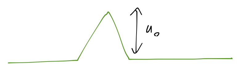
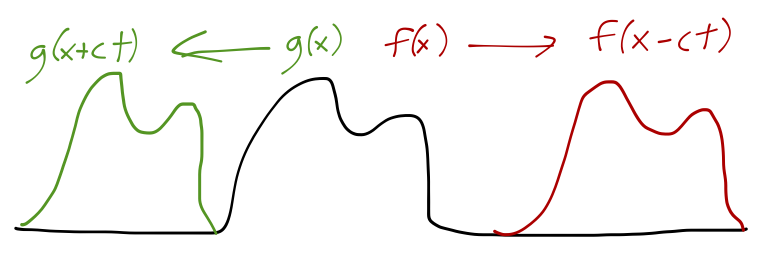
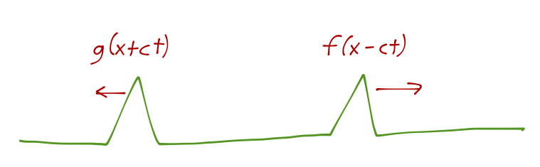
We start by introducing the odd-looking variables \xi = x - ct \\ \eta = x + ct. These are arranged to give us a sort of cancellation between mixed derivatives when we rewrite the wave equation. Here’s how it works: first we see that in terms of the new variables, x and t are given by x = \frac{1}{2} (\eta + \xi) \\ t = \frac{1}{2c} (\eta - \xi). Now notice that we can write \frac{\partial u}{\partial \eta} = \frac{1}{2} \frac{\partial u}{\partial x} + \frac{1}{2c} \frac{\partial u}{\partial t}. But now, \frac{\partial}{\partial \xi} \frac{\partial u}{\partial \eta} = \frac{1}{4} \left[ \frac{\partial^2 u}{\partial x^2} - \frac{1}{c} \frac{\partial^2 u}{\partial x \partial t} + \frac{1}{c} \frac{\partial^2 u}{\partial t \partial x} - \frac{1}{c^2} \frac{\partial^2 u}{\partial t^2} \right]. Multiplying through by -4c^2, we see that we’ve rewritten the wave equation: \frac{\partial^2 u}{\partial t^2} - c^2 \frac{\partial^2 u}{\partial x^2} = -4c^2 \frac{\partial}{\partial \xi} \frac{\partial u}{\partial \eta} = 0. What does this mean? If we temporarily write \partial u / \partial \eta = h, then the function h satisfies \partial h / \partial \xi = 0, which means that h = h(\eta). But the solution to the differential equation for u is \int h(\eta) + C; h isn’t allowed to depend on \xi, but the “constant” C can! Without actually knowing anything else, this proves that the final solution must be written in the form u = f(\xi) + g(\eta) = f(x-ct) + g(x+ct). It’s interesting to consider what this implies for an isolated disturbance along our string. We might get such a disturbance by, say, pulling on the string at x to some initial height u_0, and then letting it go, giving us something like a triangular wave:
Once we release the string, what happens? The first term f(x-ct) is a forwards-propagating wave. If we start with a particular shape f(kx) at t=0, then after some time we will find the exact same shape, but with its center translated to x' = ct. The other solution g(x+ct) is a backwards-propagating wave; its center will be translated by the same distance, but in the opposite direction.
Note that \omega/k \equiv c has units of speed, and indeed we can think of it as the speed at which a wave propagates. For the spring system, the wave speed was c = \sqrt{E/\rho}, which makes sense: the longitudinal waves along the spring will travel faster if the elastic modulus is bigger, but slower if the spring is heavier. This is the same c that appears in the wave equation itself.
16.1.2.1 fix notation here
So, what happens to the string when we create a triangular wave at x=0? The initial triangular wave u(x,0) must be written as u(x,0) = f(kx) + g(kx). Since we’re releasing the string at rest, we also want \dot{u}(x,0) = 0, or \dot{u}(x,0) = -\omega f'(kx) + \omega g'(kx) = 0. Combining these two equations we must have f(kx) = g(kx). So the initial triangular wave must be the sum of two smaller triangular waves, which will propagate away in opposite directions:
Let’s think about a few more examples of wave propagation.
16.1.3 Solving the wave equation
Back to the wave equation in its original form: \frac{\partial^2 u(x,t)}{\partial t^2} = c^2 \frac{\partial^2 u(x,t)}{\partial x^2}. We can use the technique of separation of variables, which is a standard trick in the math of partial differential equations, in order to find the general solution to the wave equation. We suppose that we can rewrite the full solution u(x,t) in the following “separated” form: u(x,t) = X(x) T(t). Then, plugging back into the wave equation, we find X(x) \ddot{T}(t) = c^2 X''(x) T(t) \\ \frac{1}{c^2} \frac{\ddot{T}(t)}{T(t)} = \frac{X''(x)}{X(x)}. From the point of view of x, the left-hand side here is just a constant; ditto the right-hand side in terms of t. Moreover, because the two sides are equal, the two constants are equal. In other words, if I let \frac{X''(x)}{X(x)} = -k^2. then \frac{\ddot{T}(t)}{T(t)} = -c^2 k^2, and I can now write two separate differential equations, X''(x) = -k^2 X(x) \\ \ddot{T}(t) = -c^2 k^2 T(t). This is just a pair of simple harmonic oscillator equations! We can thus immediately write down the general solution: u(x,t) = (A \cos (kx) + B \sin (kx)) (C \cos (\omega t) + D \sin (\omega t)) where \omega = ck. The constant k appearing here is called the wave number, and is positive by convention. You can verify that k has units of inverse length, as it must to make kx dimensionless. It is related to the wavelength \lambda as k = 2\pi / \lambda.
Unlike equations like the SHO, we do not find a unique answer for \omega or k. Unless we impose some other conditions, any \omega is allowed for a solution, as long as we also have k = \omega/c.