10 Orbital Mechanics
10.1 Central force motion
Now we’re finally going to apply the Lagrangian to solve some more complex and interesting mechanics problems. Our first stop will be what the book calls “Two-Body Central-Force Problems”. As a reminder, a central force is one which is spherically symmetric; for an object moving in the force field in spherical coordinates with the source at the origin, we can write it as \vec{F}_{\textrm{cent}} = F(\vec{r}) \hat{r}, so the force is always directed towards or away from the source at the center. Not all forces are central; the magnetic force is an obvious counterexample. But the electric force, gravitational force, and even the force exerted by a spring are all central forces.
Moreover, these are all conservative forces, which means that they each have a corresponding potential energy function U. In fact, for a central force, U must be independent of \theta and \phi, otherwise the force \vec{F} = -\nabla U would end up with components in those directions. So U = U(r), and similarly \vec{F} = \vec{F}(r).
Two-body, clearly, means we will be considering problems involving only two objects. This includes a number of very interesting physical systems; the motion of a planet around the sun, and the orbit of an electron around the nucleus of an atom are the most important. Of course, the solar system contains 8 planets and a swarm of smaller objects, and most atoms have many electrons, but we can still learn a lot just by considering two objects in isolation, particularly for the solar system where the gravitational pull of the Sun dominates the effects of all of the other objects.
(The hydrogen atom is a purely two-body problem, but you’ll need quantum mechanics to fully understand its properties; still, the classical setup of the two-body problem is a prerequisite for solving the quantum system.)
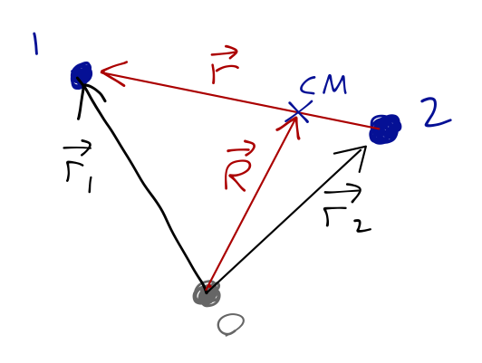
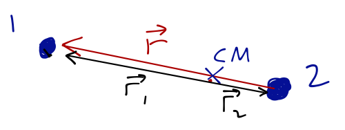
Consider two objects, labelled 1 and 2. Their masses are m_1, m_2, positions are \vec{r_1}, \vec{r_2}. We assume a conservative, central force, so potential depends only on relative distance: U(\vec{r_1}, \vec{r_2}) = U(|\vec{r_1} - \vec{r_2}|) \equiv U(r). With all of that, the Lagrangian is \mathcal{L} = \frac{1}{2} m_1 \dot{\vec{r_1}}^2 + \frac{1}{2} m_2 \dot{\vec{r_2}}^2 - U(r). Now we can pick generalized coordinates! Two objects and no constraints, so we need 6. Since \vec{r} = \vec{r_1} - \vec{r_2} appears directly in the potential, we’ll take its components as 3 of our GCs, so that leaves 3 more. Remember our second vector doesn’t have to be orthogonal to \vec{r} in our fixed coordinates, just independent of it.
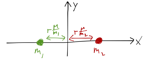
It turns out that the best choice for our remaining coordinates is the center of mass position, \vec{R}: \vec{R} = \frac{m_1 \vec{r_1} + m_2 \vec{r_2}}{M}. \vec{R} points to the center of mass (CM), on the line joining m_1 and m_2, and M = m_1 + m_2 is the total mass.
How would you guess to use this particular coordinate? As always, you need some amount of intuition, but there are two ways we might have arrived at \vec{R}:
Argue based on conservation of momentum - a collection of objects has total momentum \vec{P} = M \vec{R}, and external forces act on the CM like a point particle, \vec{F}_{\textrm{ext}} = \dot{P}.
Try it in the Lagrangian! Other combinations of \vec{r_1} with \vec{r_2} will give more complicated expressions.
10.2 Two-body central force problem
To finish our coordinate change, we need expressions for \vec{r_1} and \vec{r_2} in terms of the generalized coordinates \vec{r} and \vec{R}.
A similar construction works for \vec{r_2}, so we have \vec{r_1} = \vec{R} + \frac{m_2}{M} \vec{r} \\ \vec{r_2} = \vec{R} - \frac{m_1}{M} \vec{r} and the kinetic energy becomes T = \frac{1}{2} m_1 \left( \dot{\vec{R}} + \frac{m_2}{M} \dot{\vec{r}}\right)^2 + \frac{1}{2} m_2\left( \dot{\vec{R}} - \frac{m_1}{M} \dot{\vec{r}}\right)^2 Let’s simplify this. The \dot{\vec{R}}^2 terms are easy: T \supset \frac{1}{2} (m_1 + m_2) \dot{\vec{R}}^2 = \frac{1}{2} M \dot{\vec{R}}^2. (the \supset symbol is mathematical notation for “contains”, since I’m going to simplify piece by piece.) The \vec{r} \cdot \vec{R} terms vanish: T \supset \left(\frac{m_1 m_2}{M} - \frac{m_2 m_1}{M} \right)\dot{\vec{R}} \cdot \dot{\vec{r}} = 0 Finally, for the \vec{r}^2 terms, T \supset \frac{1}{2} \left( \frac{m_1 m_2^2}{M^2} + \frac{m_2 m_1^2}{M^2} \right) \dot{\vec{r}}^2 = \frac{1}{2} \frac{m_1 m_2}{M} \dot{\vec{r}}^2. So for the Lagrangian in our GCs, \mathcal{L} = T - U = \frac{1}{2} M \dot{\vec{R}}^2 + \frac{1}{2} \mu \dot{\vec{r}}^2 - U(r) where I’ve defined the reduced mass \mu \equiv \frac{m_1 m_2}{M} = \frac{m_1 m_2}{m_1 + m_2}. Note that if one mass is much larger than the other, the reduced mass is almost equal to the smaller mass. For example in the Earth-Sun system, M \approx M_{S}, while \mu \approx M_{\textrm{E}}.
10.2.1 Conserved quantities in the two-body problem
Since there are no external forces, the motion of the CM (as we expect) is very simple: we have \frac{\partial \mathcal{L}}{\partial \vec{R}} = 0 which tells us that M\ddot{\vec{R}} = 0. Invariance under \vec{R} gives us conservation of total momentum, M \dot{\vec{R}} = \dot{\vec{P}} = \textrm{const.} Motion under \vec{R} is ignorable - we don’t need to worry about it when solving for the dynamics of \vec{r}.
In fact, from the Newtonian point of view we know that we can work in any inertial reference frame. So if we move to the CM frame in which \dot{\vec{R}} = 0, then the variable \vec{R} vanishes completely.
Are there any conserved quantities here? Since U depends only on |\vec{r}|, you should suspect there are. Let’s work in spherical coordinates: \mathcal{L} = \frac{1}{2} \mu \left[ \dot{r}^2 + r^2 \dot{\theta}^2 + r^2 \sin^2 \theta \dot{\phi}^2\right] - U(r). First, since \partial \mathcal{L} / \partial \phi = 0, we have a conserved quantity, \frac{\partial \mathcal{L}}{\partial \dot{\phi}} = \mu r^2 \sin^2 \theta \dot{\phi} = \textrm{const}. What is this conserved momentum? You can guess from the units that it will be some sort of angular momentum. Let’s work out the total angular momentum vector of this system to see. The general formula is \vec{L} = \vec{r} \times \vec{p}, and it will add for our two objects: \vec{L} = m_1 \vec{r_1} \times \dot{\vec{r_1}} + m_2 \vec{r_2} \times \dot{\vec{r_2}}. Now we use our coordinate change above, which is simplified by working in the CM frame: we now have \vec{R} = 0. Plugging in, we find \vec{L} = \frac{m_1 m_2^2}{M^2} \vec{r} \times \dot{\vec{r}} + \frac{m_1^2 m_2}{M^2} \vec{r} \times \dot{\vec{r}} \\ = \mu \vec{r} \times \dot{\vec{r}}. This result is true in any coordinate system, since it’s a vector equation. If we expand out in spherical coordinates, using the standard result \dot{\vec{r}} = \dot{r} \hat{r} + r \dot{\theta} \hat{\theta} + r \sin \theta \dot{\phi} \hat{\phi}, (note that |\dot{\vec{r}}|^2 matches our spherical kinetic energy above!), then \vec{L} = \mu \vec{r} \times \dot{\vec{r}} = \mu \left| \begin{array}{ccc} \hat{r} & \hat{\theta} & \hat{\phi} \\ r & 0 & 0 \\ \dot{r} & r \dot{\theta} & r \sin \theta \dot{\phi} \end{array} \right| = -\mu r^2 \sin \theta \dot{\phi} \hat{\theta} + \mu r^2 \dot{\theta} \hat{\phi}. This doesn’t quite match on to our conserved quantity, but that’s partly a trick of the fact that the angular unit vectors themselves change with time in a spherical coordinate system. If you switch to a more stable Cartesian vector coordinate system, you’ll find that the conserved quantity \partial \mathcal{L}/\partial \dot{\phi} that we found above is exactly L_z, the z-component of this angular momentum vector.
Turning to the other angle \theta, the Euler-Lagrange equation is \frac{\partial \mathcal{L}}{\partial \theta} = \frac{d}{dt} \left( \frac{\partial \mathcal{L}}{\partial \dot{\theta}} \right) \\ \mu r^2 \sin \theta \cos \theta \dot{\phi}^2 = \frac{d}{dt} \left( \mu r^2 \dot{\theta} \right). This is less obviously enlightening, since both sides are non-zero. But we can make progress with a clever change of coordinates. (If you’re not happy with this method, you can go back to writing out the components of \vec{L} in Cartesian vector coordinates; you should find, after some painful algebra, that this condition gives you the same answer our coordinate-change argument does.)
Why should we expect another symmetry to be buried in this problem? Because the potential only depends on the distance between the two particles, r; the physics should be invariant under both rotational angles. In fact, this means that we are free to rotate our coordinate system around to change the initial angle \theta_0 describing the vector \vec{r}. If we choose \theta_0 = \pi/2 then the second Euler-Lagrange equation becomes, at t=0, 0 = \frac{d}{dt} \left(\mu r^2 \dot{\theta}\right) This reveals the second invariant, which is another component of angular momentum - from above, the L_\phi component in spherical coordinates. In fact, there are no free components of angular momentum left: with \theta_0 = \pi/2 our other conserved quantity is L_\theta, and there is no L_r component. So we have found that total angular momentum \vec{L} is conserved in this system.
Now, the problem with what we’ve just done is that we needed \theta = \pi/2, but we only get \theta_0 = \pi/2 from our choice of coordinates; our arguments only work if \theta doesn’t evolve in time. Expanding out the \ddot{\theta} equation of motion gives 0 = 2\mu r \dot{r} \dot{\theta} + \mu r^2 \ddot{\theta}, so everything works out as long as we do a second rotation of our coordinates to set \dot{\theta}_0 = 0 as well. We are free to do these two fixed rotations, thanks to spherical symmetry! The first puts the initial position \theta_0 of the masses in the equatorial plane, and the second rotation puts their initial velocities in the same plane.

An alternative and more physical way to see the validity of this approach is to remember that \vec{L} = \mu \vec{r} \times \dot{\vec{r}}. The cross product means that \vec{L} is perpendicular to both \vec{r} and \dot{\vec{r}}. If \vec{L} is conserved, as we have found, then both \vec{r} and \dot{\vec{r}} lie in a fixed plane perpendicular to \vec{L}. So it’s valid to constrain the motion entirely to a plane.
With \theta now fixed, the only dynamical coordinates we have left are the polar coordinates r and \phi. We can simplify further, since the Euler-Lagrange equation for \phi yielded a constant of the motion, \mu r^2 \dot{\phi} = L_z = \textrm{const}. Let’s write the third and final Euler-Lagrange equation, for r: \mu \ddot{r} = \mu r \dot{\phi}^2 - \frac{dU}{dr}. We can use L_z to substitute in to this equation for \dot{\phi}, finding \mu \ddot{r} = \frac{L_z^2}{\mu r^3} - \frac{dU}{dr}. This is now a differential equation purely in terms of r(t). Hopefully now you can appreciate the power of finding constants of the motion! Although the dynamics of the system gives us motion in both r and \phi, by identifying L_z as a constant we can reduce the problem to solving a single differential equation for r(t); once we have this, we simplify have to plug back in to the definition of L_z and integrate to find \phi(t).
10.3 Equation of orbit
Some more comments are in order about this equation. If there is no angular momentum, then we only have the second term, which is just the force acting in the radial direction, F = -\nabla U. The extra term we have picked up can be identified as a centrifugal force term.
Notice that since the centrifugal term is just a simple power law in r, it would be very easy to write it as the derivative of something. This allows us to define the effective potential U_{\textrm{eff}}(r) = U(r) + \frac{L_z^2}{2\mu r^2}, and then the equation of motion for r is just \mu \ddot{r} = -\frac{dU_{\textrm{eff}}}{dr}. Is this really still a potential energy function, though? The answer is “sort of”. If we pretend that we’re just solving a one-dimensional problem for a particle with mass \mu moving under the effect of U_{\textrm{eff}}, then the total energy of the system is E = T + U_{\textrm{eff}} = \frac{1}{2} \mu \dot{r}^2 + \frac{L_z^2}{2\mu r^2} + U(r) \\ = \frac{1}{2} \mu \dot{r}^2 + \frac{(\mu r^2 \dot{\phi})^2}{2\mu r^2} + U(r) \\ = \frac{1}{2} \mu \dot{r}^2 + \frac{1}{2} \mu r^2 \dot{\phi}^2 + U(r) which is exactly the total energy from our original two-dimensional Lagrangian. In a sense, we’ve just pushed one of our kinetic energy terms into the potential energy for r instead. Thus, the six-dimensional motion of two objects interacting with a central force has been reduced by symmetry considerations all the way down to this equivalent one-dimensional problem.
However, there is one very important problem with interpreting U_{\textrm{eff}} as a potential energy: do not try to substitute the expression \mu r^2 \dot{\phi} = L_z into the two-dimensional Lagrangian and then solve the Euler-Lagrange equation for r. You will get the wrong answer! We can only substitute for \dot{\phi} in the equations of motion, after the fact. The Lagrangian was derived assuming all the variables are independent, and solving one of the equations of motion and then trying to plug back in will not work.
In other words, it’s true that dL_z/dt = 0 since it’s a constant of the motion, but dL_z / dr \neq 0, and the latter will cause problems at the level of the Lagrangian. (We are done with the Lagrangian now that we have the equation for r(t), but I’m mentioning this to avoid a conceptual pitfall.)
10.3.1 Example: motion with no forces
In case this shuffling around of kinetic and potential energies looks suspicious to you, let’s do an example with no forces at all to see what’s really going on.
Suppose U = 0, and let’s take m_2 \gg m_1 (which means \mu \approx m_1) and look at the motion of m_1. Obviously, we know that with no forces, it will just travel past m_2 in a straight line:
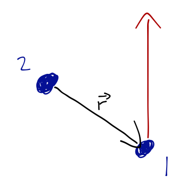
Nevertheless, if we write the two-body equation of motion in our polar coordinates, we find a non-zero (effective) potential energy: U_{\textrm{eff}} = \frac{L_z^2}{2\mu r^2} so the equation of motion is m_1 \ddot{r} = -\frac{dU_{\textrm{eff}}}{dr} = \frac{L_z^2}{m_1 r^3}. Even though we started with no potential, there is an apparent “centrifugal” force! We shouldn’t be surprised by this, because in fact r is a lousy coordinate for this problem. We know that r changes as the particle moves along the line; it decreases to a minimum as m_1 approaches m_2, and then starts to increase again. The equation for r is complicated because it should be! (I won’t go through the solution of this differential equation for r(t), since we already know what the motion should look like.)
One more note: despite my warning above about Lagrangian substitution, remember that from the perspective of the one-dimensional problem, it’s perfectly consistent to treat U_{\rm eff} as an effective potential energy. So we can write the Lagrangian as \mathcal{L} = \frac{1}{2}\mu \dot{r}^2 - \frac{L_z^2}{2\mu r^2}, and the equation of motion we find will be correct. What is incorrect is to start with the 2-D Lagrangian, and make this substitution: \mathcal{L} = \frac{1}{2} \mu (\dot{r}^2 + r^2 \dot{\phi}^2) \neq \frac{1}{2} \mu \dot{r}^2 + \frac{L_z^2}{2\mu r^2}, which clearly gives the wrong sign.
10.3.2 Example: spring force
Let’s do a more complete example to see everything at work here. Suppose we connect two masses m_1 and m_2 by a spring with constant k and natural length \ell, and then slide them across a horizontal frictionless table: the situation is depicted below.
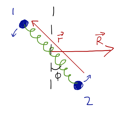
Before I go to the effective potential, let’s consider what the two-dimensional Euler-Lagrange equations look like. They are easily seen to be: \mu \ddot{r} = \mu r \dot{\phi}^2 - k(r-\ell) \\ \mu r^2 \dot{\phi} = \textrm{const} = L_z. There are two special cases we can consider here. If L_z = 0 (\dot{\phi} = 0), then the two masses are just translating but not spinning. The equation of motion becomes \mu \ddot{r} = -k(r-\ell) which is just the standard simple harmonic oscillator equation we would have had if the spring system was at rest. (In fact, it is at rest in the CM frame!)
What about equilibrium solutions, where r = \textrm{const}? If r is a constant then the \phi equation tells us that \dot{\phi} = \textrm{const}, and from the other equation since \ddot{r} = 0 we have k(r-\ell) = \mu r \dot{\phi}^2 This is just “spring force = centripetal force”, as the two masses revolve in simple circular motion about the CM.
After-lecture aside: what is the equilibrium value of r here? We can solve the equation to find (k - \mu \dot{\phi}^2) r = k\ell \Rightarrow r = \frac{\ell}{1 - (\mu/k) \dot{\phi}^2}. This is a funny-looking result, since it seems to imply that r can change signs if we spin the system fast enough! However, that’s not really the case. If we begin by considering \dot{\phi} relatively small, so the denominator remains between 0 and 1, then this expression makes sense: as \dot{\phi} increases, the equilibrium value of r is pushed out towards values larger than \ell, where it would be if there was no rotational motion.
However, remember that \dot{\phi} is not arbitrary here! This is not an initial condition, it’s an equilibrium solution. Going back to the equation for angular momentum, we recall that \dot{\phi} = \frac{L_z}{\mu r^2}. So there is a stabilizing effect: as r increases, the required value of \dot{\phi} to reach equilibrium is suppressed. In fact, we can plug back in to the equation above to find the equilibrium r in terms of the angular momentum, and there will always be a solution no matter how large we make the initial L_z. (The equation is a quartic polynomial so I won’t try to write out the solution here, but Mathematica will give it to you if you ask nicely.)
For the more general case, the easiest way to approach the problem is in terms of the “effective potential” we defined above! For the spring, we find that U_{\textrm{eff}} = \frac{1}{2} k(r-\ell)^2 + \frac{L_z^2}{2\mu r^2}. So we have a quadratic term and a 1/r^2 term, which is known as the centrifugal barrier. It’s easy to sketch what the shape of the potential will look like for various choices of L_z:
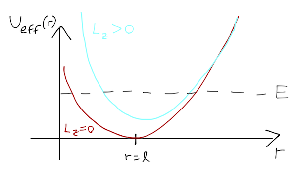
Why is plotting U_{\textrm{eff}} useful? Remember this is completely equivalent to the 1-D problem of finding the motion of r in such a potential. Since we know total energy E = T + U_{\textrm{eff}} is conserved, we can draw lines for a given E.
Whenever E = U_{\textrm{eff}}, we must have T = 0, and the particle can never reach larger values of U - these are the turning points. So without solving the motion, we can see that if we start our system with greater E, it will undergo oscillations with larger amplitude. For any E the particle is always “trapped”; it always has a minimum and maximum r.
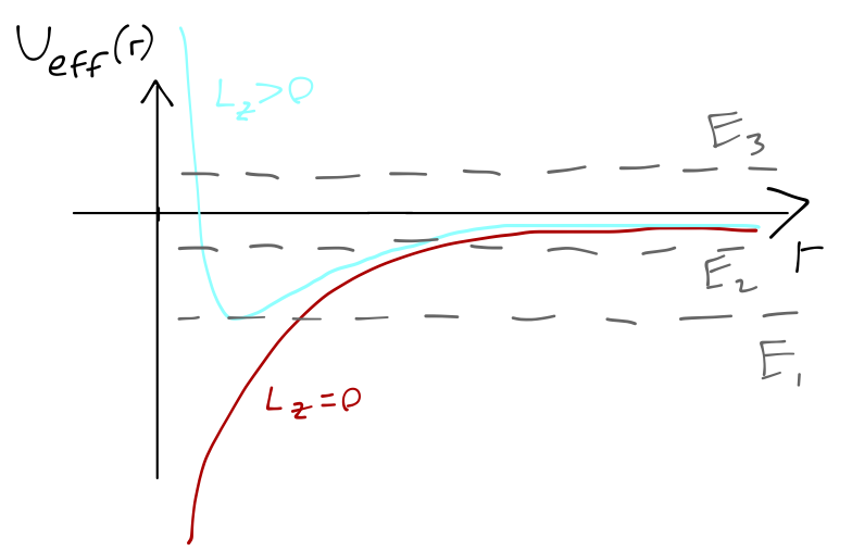
The spring example doesn’t turn out to be too interesting; the motion is always some sort of oscillation between minimum and maximum values of r. Let’s instead turn to the more interesting case of gravitational interaction. Suppose we want to solve for the motion of a comet of mass m under the influence of the Sun’s gravity. The potential is U_{\textrm{eff}} = -\frac{GM_s m}{r} + \frac{L_z^2}{2\mu r^2}. We can sketch what this looks like, with or without angular momentum:
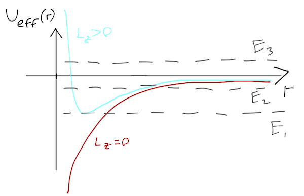
Now the motion (when L_z > 0) is much more interesting. I’ve drawn three energy levels on the potential plot. E_1 corresponds to a stable, circular orbit, as in the spring example. The orbit of E_2 is also stable; there is a minimum and maximum value of r, which the comet will move between in some way. Finally, E_3 is unstable; there is a minimum value of r, but no maximum.
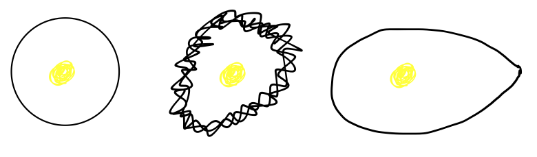
We can learn a lot just from drawing this plot and thinking about the turning points, but this approach doesn’t give us the details of what is happening in the middle of the orbit. For example, we need to dig further to answer the simple question: what is the shape of an orbit with a given total energy E?
The answer is obvious if r is constant: we get a circular orbit. But if r is varying with time, just knowing the minimum and maximum possible values doesn’t tell us much about what happens in the middle:
10.4 Orbital motion
Specializing from the general two-body problem to a 1/r effective potential, U_{\textrm{eff}} = \frac{L_z^2}{2\mu r^2} - \frac{\gamma}{r}. where for gravity \gamma = Gm_1 m_2, one can solve for the equation of orbit: r(\phi) = \frac{c}{1+\epsilon \cos \phi}. Now that we have the equation in hand, let’s try to interpret it.
An immediate and very interesting observation we can make from the equation of orbit is that r(\phi) is periodic as \phi \rightarrow \phi + 2\pi. Obviously the simplest orbit occurs for \epsilon = 0, in which case we simply have r(\phi) = c, i.e. a circular orbit. But for more complicated orbits, this periodicity means that the orbit closes: r(0) and r(2\pi) are the same point in space. (This didn’t have to be true!)
An orbit which is 2\pi periodic in \phi is called stable, since we can draw it as a simple closed curve in space. Circular orbits are always trivially stable, since they don’t depend on \phi.
(Fun fact: one of the key assumptions that we made to end up with a stable orbit was that the potential goes as U \sim 1/r. In fact, there are only two types of potentials which give stable orbits other than circles: this, and the spring potential U \sim r^2. This fact is known as Bertrand’s Law.)
What does this orbit look like for 0 < \epsilon < 1? I can sketch the denominator c/r(\phi):
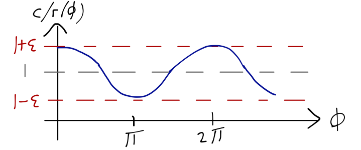
So for \epsilon < 1, we have a bound orbit, which oscillates between the values r_{\textrm{min}} = \frac{c}{1+\epsilon},\ \ r_{\textrm{max}} = \frac{c}{1-\epsilon}. The coordinates where minimum and maximum r occur are known as periapsis and apoapsis, respectively (remember: “a” is further away.) If the orbit is around the sun, you’ll see the terms perihelion and aphelion instead; for the Earth, it’s perigee and apogee.
A quick note: remember that we got rid of an arbitrary phase \delta in our derivation. We can see now that physically, the choice \delta = 0 amounts to rotating our coordinate system so that periapsis occurs at \phi = 0, on the positive x-axis. This is fine as long as we’re using arbitrary coordinates, but if we have multiple two-body systems in the same coordinates (like the planets in the solar system), then we need to include the periapsis phase \delta in order to describe their motion correctly. We would do this by replacing \phi with \phi - \delta in the equation of orbit.
What does the orbit look like in space? Periapsis is at \phi = 0 and apoapsis at \phi = \pi, and the radius varies smoothly between the two, so we end up with an ellipse:
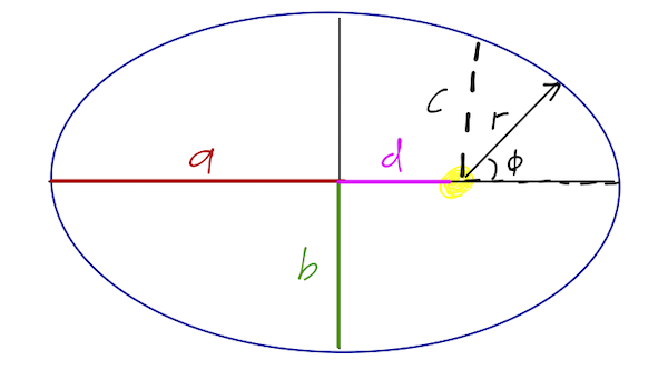
The book switches to Cartesian coordinates at this point, but I say why bother? You can already see this is an ellipse, and we can work out its properties very easily from the equation of orbit. The parameter \epsilon is called the eccentricity of the ellipse; a more eccentric orbit is more oblong. (We already saw that \epsilon = 0 is a circle.)
Just as the shape of a circle is determined by its radius, the shape of an ellipse is determined by the major and minor axes, which are like the diameter in the long and short directions. Half of the axis length is called the semimajor axis (a) or semiminor axis (b). From the equation of orbit, we can identify c on our plot as the radius at \phi = \pi/2, which means the distance to the ellipse vertically above or below the origin. Finally, I’ve labelled the offset between the center of the ellipse and our origin (the CM location) as d.
We can write formulas for all of these lengths, but they’re all easy to derive from the equation of orbit, as we will now see.
Once we have length a, it’s straightforward to find d in a similar way: d = a - r_{\textrm{min}} \\ = \frac{c}{(1-\epsilon^2)} - \frac{c}{1+\epsilon} \\ = \frac{c - c + c \epsilon}{(1-\epsilon^2)} \\ = \frac{c\epsilon}{(1-\epsilon^2)} \\ = \epsilon a. The hardest length to find is b. There are a few ways to do it: the most direct is to write the equation for a straight vertical line y = -d in polar coordinates as r \sin \phi = -d, and then solve for where it intersects the ellipse, and then use b^2 + d^2 = r^2. However, this is much easier if you remember a special property of an ellipse. The two points along the semimajor axis d from the center (one of which is the CM!) are called the foci of the ellipse, and any point on the ellipse is a total distance of 2a from the two foci. This is one of the definitions of an ellipse. (You can use a string of length 2a anchored at the foci to draw an ellipse, in fact.)
Because of this fact, we know that at the bottom of the ellipse, \sqrt{d^2 + b^2} + \sqrt{d^2 + b^2} = 2a \\ 4a^2 = 4(b^2 + d^2) \\ b = \sqrt{a^2 - d^2} \\ = \sqrt{a^2 - \epsilon^2 a^2} \\ = \frac{c}{\sqrt{1-\epsilon^2}}. Notice that the ratio of the two axes is \frac{b}{a} = \sqrt{1-\epsilon^2} which is another way to define an ellipse of eccentricity \epsilon.
10.4.1 Orbital period
So now we can draw the orbit, but by going to r(\phi) we’ve lost information about time evolution. In particular, how do we know the orbital period, i.e. how long it takes the object to return to the starting point? Taylor does the standard “sweeping out areas” argument, but I’ll show you another way using the chain rule.
We can write the orbital velocity as: \dot{r} = \frac{dr}{d\phi} \frac{d\phi}{dt} \\ = \frac{c\epsilon \sin \phi}{(1+\epsilon \cos \phi)^2} \dot{\phi} \\ = r^2 \frac{\epsilon \sin \phi}{c} \frac{L_z}{\mu r^2} \\ = \epsilon \sin \phi \sqrt{\frac{\gamma}{\mu c}}, remembering that c = L_z^2 / (\gamma \mu). Now, \dot{r} = dr/dt, so we can reorganize into dt = dr \sqrt{\frac{\mu c}{\gamma}} \frac{1}{\epsilon \sin \phi}. We also know that dr = d\phi \frac{c\epsilon \sin \phi}{(1+\epsilon \cos\phi)^2} so combining and integrating both sides, t = \int_{\phi_i}^{\phi_f} d\phi \frac{c\epsilon \sin \phi}{(1+\epsilon \cos \phi)^2} \sqrt{\frac{\mu c}{\gamma}} \frac{1}{\epsilon \sin \phi} \\ = c^{3/2} \sqrt{\frac{\mu}{\gamma}} \int_{\phi_i}^{\phi_f} \frac{d\phi}{(1+\epsilon \cos \phi)^2}. Note that this is a nice expression; it will give us not just the orbital period, but the time taken for the orbit to evolve between any two angles \phi_i and \phi_f. To get the orbital period, we just set the limits to 0 and 2\pi. The integral takes some work, but if you do some clever substitutions or ask Mathematica nicely, you will find (for 0 < \epsilon < 1): \tau = c^{3/2} \sqrt{\frac{\mu}{\gamma}} \frac{2\pi}{(1-\epsilon^2)^{3/2}} or for an object moving around the Sun under gravity, where \gamma = G m_1 m_2 \approx G \mu M_{\odot}, \tau^2 = \left(\frac{c}{1-\epsilon^2}\right)^3 \frac{4\pi^2}{G M_{\odot}} = \frac{4\pi^2}{GM_\odot} a^3.
Note: as was pointed out to me in class, this equation is often written with the sum of the solar and planet masses in the denominator. Let’s see where that comes from: let m be the mass of the planet. Then the reduced mass is \mu = mM_{\odot} / (m + M_{\odot}), and we have in the orbital period formula \frac{\mu}{\gamma} = \frac{m M_{\odot}}{(m + M_{\odot}) G m M_{\odot}} = \frac{1}{G(m+M_{\odot})}, giving instead \tau^2 = \frac{4\pi^2}{G(m+M_{\odot})} a^3. which is the more correct formula.
The correction due to including m is pretty small in practice, but not always totally negligible. The mass of the Earth is about 3 \times 10^{-6} M_{\odot}, so the approximate formula above gives an orbital period which is off by about 45 seconds from the correct length of a year. On the other hand, Jupiter (the heaviest planet in the solar system) has a mass of 0.00095 times M_{\odot} and a 12-year orbital period, so using M_{\odot} instead of m + M_{\odot} would give you the wrong period by 2 days. Close enough for physics homework, but if you’re launching a probe to Jupiter you probably care about the difference!
We have now derived several important facts about bound orbits, and in fact, we have at this point proved all three of Kepler’s Laws of planetary motion:
- Planets orbit in ellipses, with the Sun at one focus.
- Angular momentum L_z is conserved (Kepler would say this differently, “equal areas swept out in equal times”.)
- The period of the orbit is given by the formula we just found.
The point I’m trying to emphasize is that from a modern point of view, Kepler’s laws are all simple consequences of the two-body problem and the equation of orbit that we found. So if you remember one thing, remember that equation!
10.5 Unbound orbits and energy
Before we move on to \epsilon \geq 1, let’s work through an example of how what we’ve learned so far can be applied!
10.5.1 Example: satellite orbit
(Note: this is actually a problem from Taylor, although I’m going to not write the number explicitly just to make it harder to find on Google for enterprising students…)
Here we consider the motion of a satellite orbiting the Earth, and we’re given two facts: its closest approach to the Earth is r_P = 250 km and its speed at that point is v = 8500 m/s. Can we find the eccentricity of its orbit and its furthest distance r_{\rm max}?
First of all, this is obviously a case where one object is much, much heavier, so I’ll use the approximations \mu \approx m and m + M_e \approx M_e, where m is the satellite mass and M_e is the Earth’s mass. We have to determine c and \epsilon to know the full orbit, and we are given two quantities so that should be enough. But we need to find how the speed is determined first!
The brute-force approach would be to use the chain rule again, with the general expression v = \sqrt{\dot{r}^2 + r^2 \dot{\phi}^2} along with the equation of orbit. We’ll do this shortly because it will give us a nice and general formula, but at perigee there are a couple of simpler methods we can try.
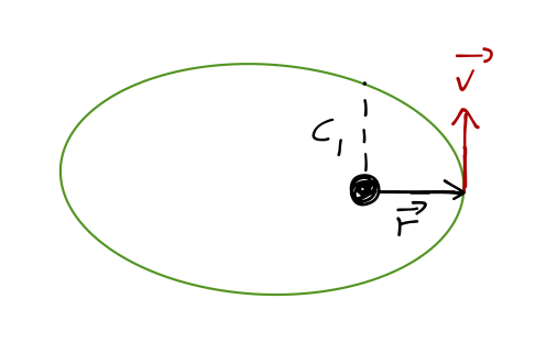
First, we can argue based on angular momentum. The direction of the velocity vector \vec{v} = \dot{\vec{r}} is always tangent to the orbit itself, and at perigee \vec{r} itself is perpendicular to the orbit:
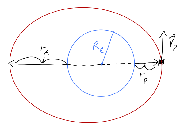
This means that it’s easy to directly evaluate the angular momentum, L_z = m|\vec{r} \times \vec{v}| = mr_{\rm min} v_P where v_P is the speed at perigee. (In general the cross product gives \sin \theta where \theta is the angle between the vectors, but since they’re perpendicular here that’s just 1.) We can plug in to the definition of c: c = \frac{L_z^2}{\gamma \mu} = \frac{(m r_{\rm min} v_P)^2}{Gm^2 M_e} = \frac{r_{\rm min}^2 v_P^2}{GM_e}. From the sketch above, we note that r_{\rm min} is not just r_P - that’s the distance above the surface of the Earth! So r_{\rm min} = r_P + R_e \approx 6650\ {\rm km}. We could just plug in numbers now, but as a nice little shortcut (which Taylor suggests), we can recognize that the combination G M_e / R_e^2 = g, so c = \frac{r_{\rm min}^2 v_P^2}{g R_e^2} \\ = \left(\frac{6650\ {\rm km}}{6400\ {\rm km}}\right)^2 \frac{8.5\ {\rm km/s} \times 8500\ {\rm m/s}}{10\ {\rm m/s^2}} \\ = 7800\ {\rm km}. We can go from here directly to \epsilon through the equation of orbit: r_{\rm min} = \frac{c}{1+\epsilon} \\ \epsilon = \frac{c}{r_{\rm min}} - 1 = \frac{7800\ {\rm km}}{6650\ {\rm km}} - 1 = 0.17. Finally, we can use this to find the distance above the Earth’s surface at apogee: r_{\rm max} = \frac{c}{1-\epsilon} = \frac{7800\ {\rm km}}{0.83} = 9400\ {\rm km} \\ r_{A} = r_{\rm max} - r_e = 3000\ {\rm km}. ### Unbound orbits
Let’s come back to the case \epsilon \geq 1, which should be perfectly good solutions - our equation of orbit derivation only required that \epsilon \geq 0. Let’s start at the boundary, with \epsilon = 1. Then the orbit is r(\phi) = \frac{c}{1+\cos \phi}. Again, closest approach is still at \phi = 0 by construction, but now we see a divergence: the radius becomes infinite at \phi = \pm \pi. This must be an unbound orbit; the two objects can escape each other completely (infinite separation.)
What sort of shape is this? It’s easier to see in Cartesian coordinates. We know that x = r \cos \phi, so r = \frac{c}{1+x/r} \\ = \frac{cr}{r+x} \\ r+x = c \\ r^2 = (c-x)^2 = c^2 - 2cx + x^2 \\ x^2 + y^2 = c^2 - 2cx + x^2 \\ x = \frac{c}{2} - \frac{y^2}{2c}. This is a parabola, opening to the left along the x-axis; the closest approach is at r_{\rm min} = c/2.
If we continue to increase \epsilon beyond 1, the radius goes to infinity for angles \phi < \pi. We can switch to Cartesian coordinates in a similar way, but it’s messier. I won’t go through the algebra, but I’ll simply tell you these curves are now hyperbolas.
A hyperbola looks similar to a parabola, but it has asymptotes, lines which it will never cross. This is actually one feature of conic sections that’s much easier to see in polar coordinates! The angles of the asymptotic lines are easy to read off of the equation of orbit: \cos (\phi_{\textrm{max}}) = \pm 1/\epsilon. In other words, if you draw a ray from the origin along a direction given by an angle greater than \phi_{\rm max}, it will never cross the hyperbolic orbit. For a parabolic orbit, this isn’t true; the parabola crosses every line that isn’t the x-axis itself away from r_{\rm min}.
The point of closest approach is, as always, at r_{\textrm{min}} = c/(1+\epsilon). We can sketch the set of all orbits, bound and unbound, that we’ve found:
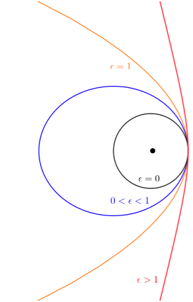
From this picture, we find an intuitive connection back to where our discussion of orbits started, namely the orbital energy. Clearly, as \epsilon increases so does the energy of the moving object; its apoapsis point moves outwards to less negative maximum values of the gravitational potential. We can confirm this intuition by going back to our energy diagram:
Now we can remember that circular orbits have the minimum possible energy, bound orbits (the ellipses) always have E < 0, and finally unbound orbits occur for E \geq 0; thus, the parabolic orbit with \epsilon = 1 must have E = 0 as well.
But how exactly does E depend on the parameters of the orbit? Let’s go back to the equation of orbit once again, and try to be more quantitative.
10.5.2 Orbital energy and angular momentum
Given a particular force law and pair of objects, the length c is determined entirely by the angular momentum L_z: c = \frac{L_z^2}{\gamma \mu}. We can reverse this equation to find L_z = \sqrt{\gamma \mu c} or for the specific case of gravity, L_z = \sqrt{Gm_1 m_2 \mu c} \\ \approx \mu \sqrt{GMc} in the usual limit where one mass is much larger than the other, so m_1 \approx \mu and m_2 \approx M. So, angular momentum (per unit mass) goes as the square root of the length c.
What about energy? We know at the turning points that the kinetic energy vanishes, so E = U_{\textrm{eff}}. Let’s work at r_{\textrm{min}}, which is the only turning point which exists for both bound and unbound orbits: E = U_{\textrm{eff}} (r_{\textrm{min}}) = - \frac{\gamma}{r_{\textrm{min}}} + \frac{L_z^2}{2\mu r_{\textrm{min}}^2} \\ = \frac{1}{2r_{\textrm{min}}} \left( \frac{L_z^2}{\mu r_{\textrm{min}}} - 2\gamma\right). From above we know that r_{\textrm{min}} = \frac{c}{1+\epsilon} = \frac{L_z^2}{\gamma \mu (1+\epsilon)}, so E = \frac{\gamma \mu (1+\epsilon)}{2L_z^2} \left( \gamma (1+\epsilon) - 2\gamma\right) \\ = \frac{\gamma^2 \mu}{2L_z^2} (\epsilon^2 - 1). The coefficient out front here is always positive. This matches our expectations; for 0 \leq \epsilon < 1, E < 0 and the orbit is bound (and is a circle or ellipse.)
We can re-express this more geometrically by substituting back in for the angular momentum L_z^2 = \gamma \mu c: E = \frac{\gamma}{2c} (\epsilon^2 - 1) or explicitly for a bound orbit, E = -\frac{\gamma}{2a}. We know this version has to be only valid for bound orbits, for two reasons: one, since \gamma and a are both positive this formula always gives a negative energy; and two, for an unbound orbit a (defined using the distance r_{\rm max}) doesn’t exist!
For gravity in the limit where one mass is much smaller than the other, we can substitute in to find E = \frac{GM\mu}{2c} (\epsilon^2 - 1) \\ = \frac{-GM\mu}{2a}.
10.6 Orbital speed and energy
One more quantity remains to derive from the equation of orbit: orbital speed. In some special cases we can use conservation of energy and angular momentum to access the speed, but let’s do the general case now.
10.6.1 Orbital speed
For a variety of applications, it’s helpful to know the instantaneous speed of the objects in orbit. We can use the equation of orbit directly: we know that v = \sqrt{\dot{r}^2 + r^2 \dot{\phi}^2} \\ = \sqrt{ \left( \frac{dr}{d\phi} \frac{d\phi}{dt} \right)^2 + r^2 \left( \frac{d\phi}{dt} \right)^2} \\ = \dot{\phi} \sqrt{ \frac{c^2 \epsilon^2 \sin^2 \phi}{(1 + \epsilon \cos \phi)^4} + \frac{c^2}{(1+\epsilon \cos \phi)^2}} \\ = \dot{\phi} \sqrt{ \frac{r^4}{c^2} \epsilon^2 \sin^2 \phi + r^2}, \\ recognizing the orbital equation for r in the first term. Recalling that \dot{\phi} = L_z / (\mu r^2), we can plug back in and simplify, taking out common factors of r and c as well: = \frac{r^2}{c} \frac{L_z}{\mu r^2} \sqrt{\frac{c^2}{r^2} + \epsilon^2 \sin^2 \phi} \\ = \sqrt{\frac{\gamma}{\mu c}} \sqrt{ \frac{c^2}{r^2} + \epsilon^2 \sin^2 \phi} \\ \approx \sqrt{\frac{GM}{c}} \sqrt{\frac{c^2}{r^2} + \epsilon^2 \sin^2 \phi}. for gravity, where \gamma \approx GM\mu. Note that for a nearly circular orbit, \epsilon \approx 0 and c \approx r, and we just have the simple formula v \approx \sqrt{\frac{GM}{r}}, corresponding to ordinary circular motion. This gives (for example) the orbital speed of the Earth about the Sun, v_E \approx 30 km/s, to good approximation.
(A word of caution: note that this is the relative speed of the two orbiting objects, since we’re using the vector \vec{r} = \vec{r_1} - \vec{r_2}! In the situation of, say, a comet orbiting the Sun where one mass is much larger and the center of mass is inside the Sun, then it’s just the speed of the comet. But for orbiting objects with comparable masses, don’t just apply this formula blindly.)
Once again, it’s particularly useful to look at r_{\rm min}, where \phi = 0: there we find v(r_{\rm min}) = \sqrt{\frac{GM}{c}} \sqrt{\frac{c^2}{r_{\rm min}^2} + \epsilon \sin (0)} \\ = \sqrt{\frac{GMc}{r_{\rm min}^2}}. This gives another, more direct way to estimate the energy of a particular orbit, if we have a small object orbiting a large one (m \ll M): then we can estimate E \approx \frac{1}{2} m v^2 - \frac{GmM}{r} \\ = \frac{1}{2} m \frac{GMc}{r_{\rm min}^2} - \frac{GmM}{r_{\rm min}} \\ = \frac{GMm}{2r_{\rm min}} \left( \epsilon - 1\right) \\ = -\frac{GMm}{2a}. You can rederive the equation for angular momentum in the same way, by writing L_z = m v_{\rm min} r_{\rm min}. We could write down new formulas for different things in terms of different length scales all day, but if you’re going to remember one thing, remember the equation of orbit, and if you’re going to remember two, then add the orbital speed; you can derive just about everything else without too much trouble.
10.6.2 Summary of orbital formulas
At this point, it’s worth summarizing some of the many formulas we’ve defined. Taylor doesn’t do a great job of this in his end-of-chapter summary in my opinion, so here’s my attempt at a more useful alternative.
All of the below are valid for the two-body problem subject to a 1/r central potential, U(r) = -\frac{\gamma}{r}. From the masses of the two bodies m_1 and m_2, we define the total mass M M = m_1 + m_2 and the reduced mass \mu \mu = \frac{m_1 m_2}{m_1 + m_2}. For the common situation of gravitational interaction with m_1 \ll m_2, we have the useful approximations m_1 \approx \mu \\ m_2 \approx M \\ \Rightarrow \gamma \approx GM\mu. Results below that use \approx are in this specific approximation.
Equation of orbit: r(\phi) = \frac{c}{1 + \epsilon \cos \phi}. Orbital speed: v(\phi) = \sqrt{\frac{\gamma}{\mu c}} \sqrt{ \frac{c^2}{r^2} + \epsilon^2 \sin^2 \phi} \\ \approx \sqrt{\frac{GM}{c}} \sqrt{\frac{c^2}{r^2} + \epsilon^2 \sin^2 \phi}. Orbital energy: E = \frac{\gamma}{2c} (\epsilon^2 - 1) \\ \approx \frac{GM\mu}{2c} (\epsilon^2 - 1) \\ \approx -\frac{GM\mu}{2a}\ \ \ {\textrm{(bound orbits only.)}} Orbital angular momentum: L_z = \sqrt{\gamma \mu c} \\ \approx \mu \sqrt{GMc} Orbital period: \tau^2 = \frac{\mu}{\gamma} 4\pi^2 a^3 \\ \approx \frac{4\pi^2}{GM} a^3. Comparison of orbital energy and angular momentum using the simple scaling relations with a and c can be particularly useful when we’re interested in orbital transfers, i.e. moving an object from one orbital path to another.
Now that we’re done deriving formulas, let’s work through a couple more examples that put our orbital model to work.
10.6.3 Example: escape velocity
You’ve probably solved this problem already last semester, but it’s nice to see how it works in our new framework: what is the minimum velocity that an object must have to escape the Earth’s gravity?
“Escape” means an unbound orbit by definition, and we know that the least energetic unbound orbital path is the E=0 orbit, namely a parabolic path with \epsilon = 1. The point of closest approach r_{\textrm{min}} = c/(1+\epsilon) = c/2 is the surface of the Earth, so c = 2R_E. Since the closest approach is at \phi = 0, using our formula for the speed, we find v_{\textrm{esc}} = \sqrt{\frac{GM_E}{2R_E}} \sqrt{\frac{4R_E^2}{R_E^2} + \sin^2 (0)} \\ = \sqrt{\frac{2GM_E}{R_E}} or plugging in the numbers M_E \approx 6 \times 10^{24} kg, R_E \approx 6.4 \times 10^6 m, we find v_{\textrm{esc}} \approx 11.2 km/s.
(By the way, the final speed of the object, plugging in to the formula for v at \phi = \pi and r \rightarrow \infty, is zero - as we should expect, since it has zero total energy.)
An interesting discussion came up in class, related to the direction of launch. If we just use standard conservation of energy arguments that don’t involve the equation of orbit, then the direction doesn’t matter at all (as long as we’re not trying to go through solid rock!) But here, I assumed that we start at r_{\rm min} of the orbit, which means the launch direction must be perpendicular to \vec{r}, i.e. towards the horizon. What is the resolution?
For any orbit, the direction of \vec{v} is always tangential to the orbit; but for a parabola, this is only perpendicular to \vec{r} at r_{\rm min}. So changing the launch direction means we must be starting at some other \phi \neq 0. If we plug in to our orbital formula for a more general \phi_0, we find (keeping \epsilon = 1:) v(\phi) = \sqrt{\frac{GM_E}{c}} \sqrt{\frac{c^2}{r(\phi_0)^2} + \sin^2 \phi_0} \\ = \sqrt{\frac{GM_E}{c}} \sqrt{(1 + \cos \phi_0)^2 + \sin^2 \phi_0} \\ = \sqrt{\frac{GM_E}{c}} \sqrt{2(1 + \cos \phi_0)} \\ = \sqrt{\frac{GM_E}{2r(\phi_0)}}, using the equation of orbit once more at the end. So since r(\phi_0) is always R_E, changing the launch angle does not change our result for the initial speed - we find the same escape velocity, exactly as conservation of energy predicts! What does change is the scale factor c, and thus the shape of the trajectory that our object will follow as it’s escaping.
10.6.4 Example: garbage disposal
Suppose we wanted to launch a rocket filled with nuclear waste off the Earth. Would it cost less energy to send the rocket into the Sun, or to send it completely outside the solar system? (The energy to get into Earth orbit is the same in either case, so we’ll work assuming that we start having already escaped Earth’s gravity well.)
Let’s consider the second case first. As above the escape velocity from radius r_E (the position of the Earth relative to the Sun) is v_{\textrm{esc},\odot} = \sqrt{\frac{2GM_\odot}{r_E}} = \sqrt{2} v_{E} where v_E = 29.8 km/s is the speed of the Earth relative to the Sun.
Since we’re launching out of the solar system, it doesn’t matter which way we send the waste; the most efficient direction is with the motion of the Earth. The velocity u relative to the Earth must then be u = (\sqrt{2} - 1) v_{E} \approx 0.41 v_{E} = 12.2\ \mbox{km/s}. Now, back to the other option: launching into the Sun. Keeping in mind that we want to minimize our total expenditure of energy, what trajectory should we send the rocket on? Since there are multiple possible orbits we may want to consider, we should frame this question in terms of orbital energy. The initial orbital energy E_i (once the rocket has escaped the Earth, which it will always have to do) is E_i = -\frac{GM_E m}{2r_E} taking the Earth to be approximately a circular orbit with radius a = r_E. We then want to put our rocket on a new orbit that satisfies two criteria:
- The orbit passes inside the Sun, which implies that r_{\rm min} \leq R_{\odot}, where R_{\odot} is the Sun’s radius;
- The energy difference \Delta E = E_f - E_i to enter our new orbit is as small as possible.
From the equation of orbit, r(0) = \frac{c}{1+\epsilon} = R_\odot \\ r(\pi) = \frac{c}{1-\epsilon} = r_E. We can write r_E - R_\odot = \frac{2c\epsilon}{1-\epsilon^2} \\ r_E + R_\odot = \frac{2c}{1-\epsilon^2} so \epsilon = \frac{r_E - R_\odot}{r_E + R_\odot} \approx 0.991 and c = r_E (1-\epsilon) = 0.009 r_E. From above, the speed of the rocket at the Earth must be v = \sqrt{\frac{GM_\odot}{c}} \frac{c}{r_E} = \sqrt{\frac{0.009 GM_\odot}{r_E}} \approx 2.8\ {\rm km/s}. Unfortunately for us, the Earth is already moving about the Sun, with an orbital velocity of 29.8 km/s. So we have to launch in the opposite direction of the Earth’s motion with a speed of about u=27.0 km/s relative to the Earth! Thus, launching out of the Solar System is (by far!) the more energy-efficient option; sending it into the Sun requires more than twice the speed and thus more than four times as much kinetic energy.
10.7 Flybys and orbital transfers
Before we wrap up with orbital mechanics and gravity, there are a couple more applications worth discussing.
10.7.1 Flyby assists
Also known as the gravitational slingshot! This is an application of unbound orbits, regularly used by NASA to speed up trips to the outer solar system.
For a flyby assist described by an unbound orbit, the important thing to note here is that the incoming and outgoing speed are identical, so v_i = v_f. We could have guessed this from the start, because the interaction with a planet conserves total energy E. So how is this an assist? Consider a hyperbolic orbit of a spacecraft around Venus:
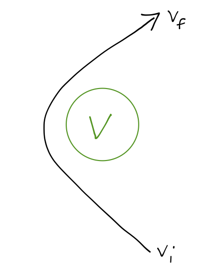
Although the final speed is unchanged in the planet-spacecraft system, the direction of the velocity vector changes - and this change of direction does give an increased speed in another frame of reference, that of the Sun! If we consider the motion relative to the Sun, we have to add the relative velocity of the spacecraft to the velocity of the planet it’s flying by (Venus, in this example):
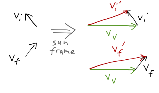
Clearly this can be used to slow down as well as speed up. There’s no problem with energy conservation - the spacecraft is taking energy from (or giving energy to) the flyby planet.
This technique is used very frequently by NASA. The Voyager missions launched in the 1980’s partly because of a rare alignment of the large outer planets - Jupiter, Saturn, Uranus, and Neptune. A series of flyby assists helped Voyagers 1 and 2 to make it all the way to Neptune in about 10 years after their launch in 1977 - it would have taken 30 years otherwise! The flyby assists helped Voyager 2 to overtake Pioneer 10 and 11, deep-space probes which were launched several years earlier.
10.7.2 Orbital transfers
As we’ve seen, we can compare the energy and angular momentum of different orbits at a glance based on the length scales a and c. This comparison is particularly important if we want to change orbits, like moving from a low-Earth orbit to a higher one, or sending an arriving probe into a stable orbit around Mars.
Let’s see quantitatively what happens to the orbit when we apply a tangential thrust - an instantaneous change in speed in the direction of motion. Suppose we start in an elliptical orbit and boost at periapsis:
We write the new speed as v_2 = \lambda v_1; \lambda is the thrust factor. Before boosting, the orbit is described by the equation of orbit, r_1 = \frac{c_1}{1 + \epsilon_1 \cos \phi}. The new orbit is described by the same equation: r_2 = \frac{c_2}{1+\epsilon_2 \cos (\phi - \delta)} Notice that a phase shift \delta has reappeared! We threw this away when solving for a single orbit, by insisting that periapsis (closest approach) is at \phi = 0. But now we’ve fixed our coordinates using orbit 1, and we’re not guaranteed that orbit 2 has periapsis at the same point! So we have to include \delta.
We can narrow our options down; since \vec{v} and \vec{r} are perpendicular before we boost, and the boost doesn’t change the direction, they stay perpendicular. This means that the new orbit is either at periapsis or apoapsis, so \delta = 0, \pi.
Changing v means changing angular momentum; remember, c \propto L_z^2. This means that c_2 = \lambda^2 c_1. We can use this and equate the two orbits at the point of the boost \phi = 0 in order to solve for \epsilon_2; I’ll skip over this because the resulting equation isn’t very enlightening, but if you do this in practice it’s important to keep track of all your plus and minus signs, including the one that can appear if \delta = \pi. Boosts at apoapsis follow the same approach, just with \phi = \pi.
We can combine orbital thrusts to change from one central-force orbit to another; this is great for e.g. going between planets in the Solar system. The most energy-efficient way to accomplish this orbital change is the Hohmann transfer, which is an elliptical orbit with periapsis and apoapsis at the two planets to be transferred between.
![]()
To execute this maneuver we have to thrust forwards, at both departure at arrival! We can make sense of this in terms of energy: the semimajor axes satisfy a_E < a < a_M for the three orbits in succession, and since E \propto -1/a, we are increasing total energy towards E=0 as a increases. (To go the other way, from Earth to Mars, then we would have to decelerate twice.)
10.8 Restricted three-body problem
You might worry that our treatment of the two-body problem has been a bit too restrictive; it’s fine for dealing with a single planet orbiting the Sun, but what about the moons orbiting those planets, or satellites moving through the Solar System?
The moment we have more than two bodies interacting, this entire framework we’ve built up goes out the window, even if there are only central forces. But we can solve a restricted three-body problem by making some big assumptions.
The restricted three-body problem is very complicated and difficult, although you now know enough about central force motion and Lagrangian mechanics to understand how to solve it. I’ll just give you the high points in lecture. If you’re interested in knowing more, many classical mechanics textbooks treat the full restricted three-body problem (although mainly graduate-level books.)
Here are the restrictions: we assume one mass is much, much smaller than the others: m_3 \ll m_1, m_2. Also, we assume m_1, m_2 are in a circular orbit. I’ll also continue to assume the motion is planar. These are strong assumptions, but close enough to describe the motion of a space probe in the Earth-Sun system, say. With that context in mind, we’ll choose gravity as our central force as well.
In a circular orbit, the angular speed of m_1 and m_2 is: \dot{\phi} = \frac{L_z}{\mu r^2} = \frac{\sqrt{\gamma \mu c}}{\mu r^2}. For this orbit, c = r and \gamma = G \mu M, so we find \dot{\phi}^2 \equiv \omega^2 = \frac{G(m_1 + m_2)}{r^3}. We can think of these masses generating a time-dependent gravitational potential for m_3, because of their mutual rotation. But it’s much easier to deal with a static potential, so instead let’s change coordinates to a rotating frame in which m_1 and m_2 are stationary.
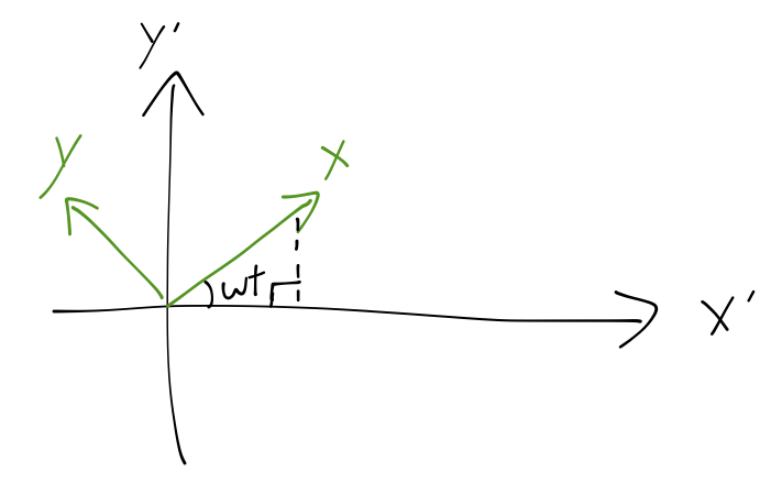
The x, y coordinates in this frame are related to the stationary ones x', y' as
x = x' \cos \omega t + y' \sin \omega t\\
y = y' \cos \omega t - x' \sin \omega t.
After some algebra, this gives a relatively nice-looking kinetic energy:
T = \frac{1}{2} m_3 (\dot{x'}^2 + \dot{y'}^2) = \frac{1}{2} m_3 \left[ (\dot{x} - \omega y)^2 + (\dot{y} + \omega x)^2\right].
The potential is just given by the distances between m_3 and the other masses, U = \frac{-Gm_1 m_3}{r_{13}} - \frac{Gm_2 m_3}{r_{23}} \\ = \frac{-Gm_1m_3}{\sqrt{(x+r\mu/m_1)^2 + y^2}} - \frac{Gm_2 m_3}{\sqrt{(x-r\mu/m_2)^2 + y^2}}, using the definition of the center of mass. Writing \mathcal{L} = T - U and going through some more algebra, the equations of motion turn out to be m_3 \ddot{x} = 2 m_3 \omega \dot{y} + m_3 \omega^2 x - \frac{dU}{dx} \\ m_3 \ddot{y} = -2 m_3 \omega \dot{x} + m_3 \omega^2 y - \frac{dU}{dy}. These are really difficult equations to solve, as you might guess. The motion is so complex that it is actually chaotic in general - infinitesimal changes in the initial conditions can completely change the trajectory. But we can at least solve for points of equilibrium where \dot{x} = \dot{y} = \ddot{x} = \ddot{y} = 0.
I won’t do this on the board, because we’d be here for a while, so I’ll skip to the answer; five equilibrium points appear from these equations of motion, known as the Lagrange points, L_1 through L_5:
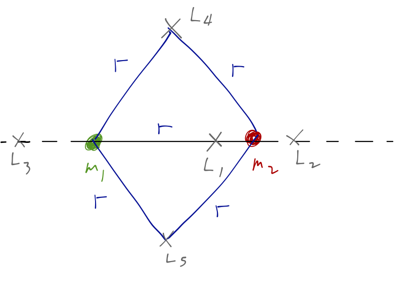
For a planet moving around the Sun, r is roughly the orbital distance, so L_4 and L_5 are on the planet’s orbital path, ahead of and behind it.
We could go further to study small oscillations around the Lagrange points; we would find L_4 and L_5 to be stable equilibria, while the other three are unstable. There tends to be an accumulation of debris at L_4 and L_5 for this reason; some other planets (Jupiter, Mars) actually have large asteroids trapped at their L_4 and L_5 points. These asteroids are known as “trojans.” (Jupiter has a lot of trojan asteroids, and when early astronomers saw two clusters of asteroids gathered on opposite sides of the planet, they named them all after characters in the Trojan War - Greeks on one side, Trojans on the other.)
NASA often makes use of the Lagrange points for spacecraft, allowing for long missions with minimal energy use. Solar observatories for example are best placed at L_3 (no moon to get in the way.) Observatories looking out into the universe (like the WMAP and PLANCK satellites observing the cosmic microwave background) sit at L_2 in the Earth’s shadow.