6 The simple harmonic oscillator
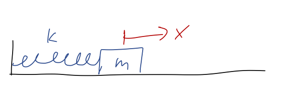
The big physics topic of this chapter is something we’ve already run into a few times: oscillatory motion, which also goes by the name harmonic motion. This sort of motion is given by the solution of the simple harmonic oscillator (SHO) equation, m\ddot{x} = -kx This happens to be the equation of motion for a spring, assuming we’ve put our equilibrium point at x=0:
The simple harmonic oscillator is an extremely important physical system study, because it appears almost everywhere in physics. In fact, we’ve already seen why it shows up everywhere: expansion around equilibrium points. If y_0 is an equilibrium point of U(y), then series expanding around that point gives U(y) = U(y_0) + \frac{1}{2} U''(y_0) (y-y_0)^2 + ... using the fact that U'(y_0) = 0, true for any equilibrium. If we change variables to x = y-y_0, and define k = U''(y_0), then this gives U(x) = U(x_0) + \frac{1}{2} kx^2 and then F(x) = -\frac{dU}{dx} = -kx which results in the simple harmonic oscillator equation. Since we’re free to add an arbitrary constant to the potential energy, we’ll ignore U(x_0) from now on, so the harmonic oscillator potential will just be U(x) = (1/2) kx^2.
Before we turn to solving the differential equation, let’s remind ourselves of what we expect for the general motion using conservation of energy. Suppose we have a fixed total energy E somewhere above the minimum at E=0. Overlaying it onto the potential energy, we have:
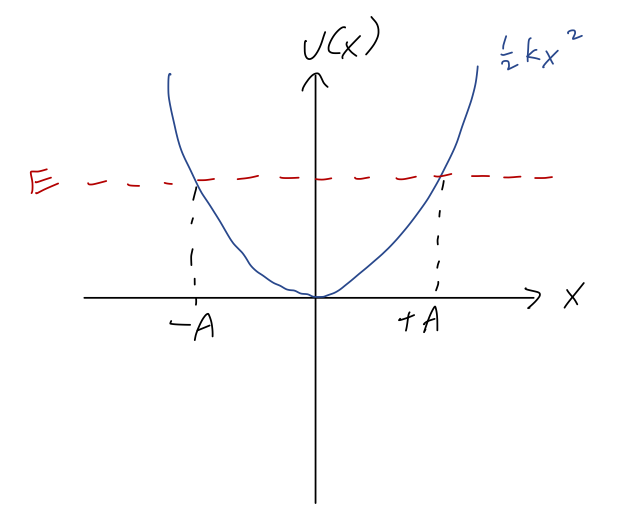
Because of the symmetry of the potential, if the value of x where E = U at positive x is U(A) = E, then we must also have U(-A) = E. Since these are the turning points, we see that A, the amplitude, is the maximum possible distance that our object can reach from the equilibrium point; it must oscillate back and forth between x = \pm A. We also know that T=0 at the turning points, which means that E = \frac{1}{2} kA^2.
This relation will make it useful to write our solutions in terms of the amplitude. But to do that, first we have to find the solutions! It’s conventional to rewrite the SHO equation in the form \ddot{x} = -\omega^2 x, where \omega^2 \equiv \frac{k}{m}. The combination \omega has units of 1/time, and the notation suggests it is an angular frequency - we’ll see why shortly.
6.1 Solving the simple harmonic oscillator
I’ve previously argued that just by inspection, we know that \sin(\omega t) and \cos(\omega t) solve this equation, because we need an x(t) that goes back to minus itself after two derivatives (and kicks out a factor of \omega^2.) But let’s be more systematic this time.
Thinking back to our general theory of ODEs, we see that this equation is:
- Linear (no functions acting on x)
- Second-order (double derivative on the left-hand side)
- Homogeneous (every term has an x or derivatives)
Since it’s linear, we know there exists a general solution, and since it’s second-order, we know it must contain exactly two unknown constants. We haven’t talked about the importance of homogeneous and second-order yet, so let’s look at that now. The most general possible homogeneous, linear, second-order ODE takes the form \frac{d^2y}{dx^2} + P(x) \frac{dy}{dx} + Q(x) y(x) = 0, where P(x) and Q(x) are arbitrary functions of x. All solutions of this equation for y(x) have an extremely useful property known as the superposition principle: if y_1(x) and y_2(x) are solutions, then any linear combination of the form ay_1(x) + by_2(x) is also a solution. It’s easy to show that if you plug that combination in to the ODE above, a bit of algebra gives a \left( \frac{d^2y_1}{dx^2} + P(x) \frac{dy_1}{dx} + Q(x) y_1(x) \right) + b \left( \frac{d^2y_2}{dx^2} + P(x) \frac{dy_2}{dx} + Q(x) y_2(x) \right) = 0 and since by assumption both y_1 and y_2 are solutions of the original equations, both of the expressions in parentheses are 0, so the whole left-hand side is 0 and the equation is true. Notice that the homogeneous part is very important for this: if there was some other F(x) on the right-hand side of the original equation, then we would get aF(x) + bF(x) on the left-hand side for our linear combination, and superposition will not work.
Anyway, the superposition principle greatly simplifies our search for a solution: if we find any two solutions, then we can add them together with arbitrary constants and we have the general solution. Let’s go back to the SHO equation: \ddot{x} = - \omega^2 x As I mentioned before, two functions that both satisfy this equation are \sin(\omega t) and \cos(\omega t). So the general solution, by superposition, is x(t) = B_1 \cos (\omega t) + B_2 \sin (\omega t).
For a general solution, we have to verify that the solutions we are adding together are linearly independent. This means simply that if we have two functions f(x) and g(x), there is no solution to the equation k_1 f(x) + k_2 g(x) = 0 except for k_1 = k_2 = 0. If there was such a solution, then we could solve for one of the functions in terms of the other, for example g(x) = -(k_1/k_2) f(x). This solution means that the linear combination C_1 f(x) + C_2 g(x) is really just the same as a single constant multiplying f(x).
If you’re uncertain about whether a collection of functions are linearly independent or not, there’s a simple test that you can do using what is known as the Wronskian determinant. For our present purposes we don’t really need the Wronskian - we know enough about trig functions to test for linear independence directly. If you’re interested, have a look at Boas 3.8.
Now, back to our general solution: x(t) = B_1 \cos (\omega t) + B_2 \sin (\omega t).
This is indeed oscillatory motion, since both \sin and \cos are periodic functions: specifically, if we wait for t = \tau = 2\pi / \omega, then x(t+\tau) = B_1 \cos (\omega t + 2\pi) + B_2 \sin (\omega t + 2\pi) = B_1 \cos (\omega t) + B_2 \sin (\omega t) = x(t) i.e. after a time of \tau, the system returns to exactly where it was. The time length \tau = \frac{2\pi}{\omega} is known as the period of oscillation, and we see that indeed \omega is the corresponding angular frequency.
To fix the arbitrary constants, we would just need to plug in initial conditions. If we have an initial position x_0 and initial speed v_0, then plugging in at t=0 the sine always vanishes, and we get the simple system of equations x_0 = x(0) = B_1 \\ v_0 = \dot{x}(0) = B_2 \omega so x(t) = x_0 \cos (\omega t) + \frac{v_0}{\omega} \sin (\omega t). This is a perfectly good solution, but this way of writing it makes answering certain questions inconvenient. For example, what is the amplitude A, i.e. the maximum displacement from x=0? It’s possible to solve for, but certainly not obvious.
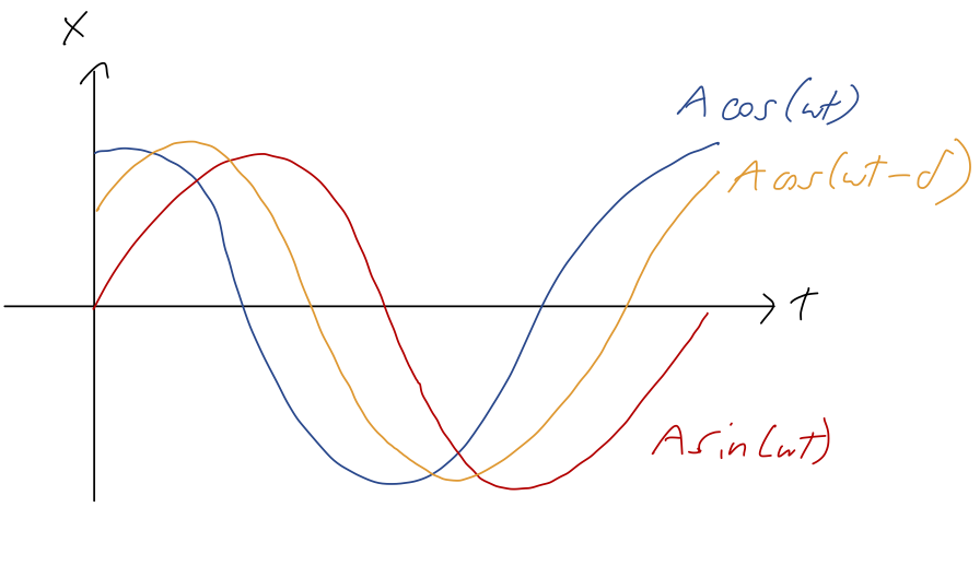
Instead of trying to find A directly, we’ll just rewrite our general solution in a different form. We know that trig identities let us combine sums of sine and cosine into a single trig function. Thus, the general solution must also be writable in the form x(t) = A \cos (\omega t - \delta) where now A and \delta are the arbitrary constants. In this form, it’s easy to see that A is exactly the amplitude, since the maximum of a single trig function is at \pm 1. We could relate A and \delta back to B_1 and B_2 using trig identities (look in Taylor), but instead we can just re-apply the initial conditions to this form: x_0 = x(0) = A \cos (-\delta) = A \cos \delta \\ v_0 = \dot{x}(0) = -\omega A \sin(-\delta) = \omega A \sin \delta
using trig identities to simplify. (We used -\delta instead of +\delta inside our general solution to ensure that there are no minus signs in these equations, in fact.) To compare a little more closely between forms, we see that if we start from rest and at positive x_0, we must have \delta = 0 and so x(t) = A \cos (\omega t) = x_0 \cos (\omega t). On the other hand, if we start at x=0 but with a positive initial speed v_0, we must have \delta = \pi/2 to match on, and so x(t) = A \cos \left(\omega t - \frac{\pi}{2}\right) = A \sin (\omega t) = \frac{v_0}{\omega} \sin (\omega t). In between the pure-cosine and pure-sine cases, for \delta between 0 and \pi/2, we have that both position and speed are non-zero at t=0. We can visualize the resulting motion as simply a phase-shifted version of the simple cases, with the phase shift \delta determining the offset between the initial time and the time where x=A:
Earlier, we found that the amplitude is related to the total energy as E = \frac{1}{2} kA^2. We can verify this against our solutions with an A in them: if we start at x=A from rest, then E = U_0 = \frac{1}{2} kx(0)^2 = \frac{1}{2} k A^2 and if we start at x=0 (so U=0) at speed v_0, then E = T_0 = \frac{1}{2} mv_0^2 = \frac{1}{2} kA^2 \\ A = \sqrt{\frac{m}{k}} v_0 = \frac{v_0}{\omega} which matches what we found above comparing our two solution forms. In fact, it’s easy to show using the phase-shifted cosine solution that E = \frac{1}{2}kA^2 always - I won’t go through the derivation, but it’s in Taylor.
Here, you should complete Tutorial 5A on “Simple Harmonic Motion”. (Tutorials are not included with these lecture notes; if you’re in the class, you will find them on Canvas.)
We’re not quite done yet: there is actually yet another way to write the general solution, which will just look like a rearrangement for now but will be extremely useful when we add extra forces to the problem. But to understand it, we need to take a brief math detour into the complex numbers.
6.2 Complex numbers
This is one of those topics that I suspect many of you have seen before, but you might be rusty on the details. So I will go quickly over the basics; if you haven’t seen this recently, make sure to review it elsewhere as well (the optional/recommended book by Boas is a good resource.)
Complex numbers are an important and useful extension of the real numbers. In particular, they can be thought of as an extension which allows us to take the square root of a negative number. We define the imaginary unit as the number which squares to -1, i^2 = -1. (Note that some books - mostly in engineering, particularly electrical engineering - will call the imaginary unit j instead, presumably because they want to reserve i for electric current.) This definition allows us to identify the square root of a negative number by including i, for example the combination 8i will square to (8i)^2 = (64) (-1) = -64 so \sqrt{-64} = 8i.
Actually, we should be careful: notice that -8i also squares to -64. Just as with the real numbers, there are two square roots for every number: +8i is the principal root of -64, the one with the positive sign that we take by default as a convention.
This ambiguity extends to i itself: some books will start with the definition \sqrt{-1} = i, but we could also have taken -i as the square root of -1 and everything would work the same. Defining i using square roots is also dangerous, because it leads you to things like this “proof”: 1 = \sqrt{1} = \sqrt{(-1) (-1)} = \sqrt{-1} \sqrt{-1} = i^2 = -1?? This is obviously wrong, because it uses a familiar property of square root that isn’t true for complex numbers: \sqrt{ab} \neq \sqrt{a} \sqrt{b} no longer works if any negatives are involved under the roots.
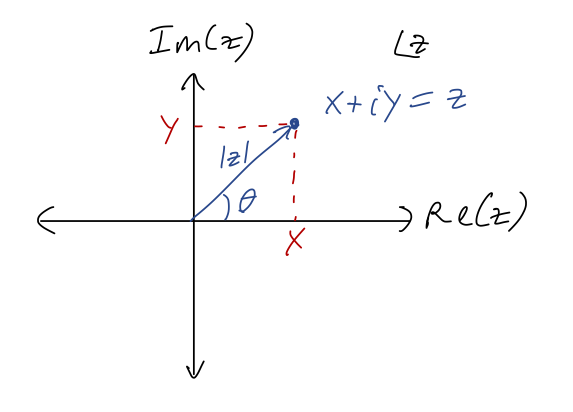
Since we’ve only added the special object i, the most general possible complex number is z = x + iy where x and y are both real. This observation leads to the fact that the complex numbers can be thought of as two copies of the real numbers. In fact, we can use this to graph complex numbers in the complex plane: if we define {\textrm{Re}}(z) = x \\ {\textrm{Im}}(z) = y as the real part and imaginary part of z, then we can draw any z as a point in a plane with coordinates (x,y) = ({\textrm{Re}}(z), {\textrm{Im}}(z)):
Obviously, numbers along the real axis here are real numbers; numbers on the vertical axis are called imaginary numbers or pure imaginary.
In complete analogy to polar coordinates, we define the magnitude or modulus of z to be |z| = \sqrt{x^2 + y^2} = \sqrt{{\textrm{Re}}(z)^2 + {\textrm{Im}}(z)^2}. We can also define an angle \theta, as pictured above, by taking \theta = \tan^{-1}(y/x) (being careful about quadrants.) This is very useful in a specific context - we’ll come back to it in a moment.
First, one more definition: for every z = x + iy, we define the complex conjugate z^\star to be z^\star = x - iy (More notation: in math books this is sometimes written \bar{z} instead of z^\star; physicists tend to prefer the star notation.) In terms of the complex plane, this is a mirror reflection across the x-axis. We note that zz^\star = (x+iy)(x-iy) = x^2 - i^2 y^2 = x^2 + y^2 so zz^\star = |z|^2 = |z^\star|^2 (the last one is true since (z^\star)^\star = z.)
Using the complex conjugate, we can write down explicit formulas for the real and imaginary parts: {\textrm{Re}} (z) = \frac{1}{2} (z + z^\star) \\ {\textrm{Im}} (z) = \frac{1}{2i} (z - z^\star). You can plug in z = x + iy and easily verify these formulas give you x and y respectively.
Multiplying and dividing complex numbers is best accomplished by doing algebra and using the definition of i. For example, (2+3i)(1-i) = 2 - 2i + 3i - 3i^2 \\ = 5 + i Division proceeds similarly, except that we should always use the complex conjugate to make the denominator real. For example, \frac{2+i}{3-i} = \frac{2+i}{3-i} \frac{3+i}{3+i} \\ = \frac{6 + 5i + i^2}{9 - i^2} \\ = \frac{6 + 5i - 1}{9 + 1} \\ = \frac{5+5i}{10} = \frac{1}{2} + \frac{i}{2}. The most important division rule to keep in mind is that dividing by i just gives an extra minus sign, e.g. \frac{2}{i} = \frac{2i}{i^2} = -2i.
Now, finally to the real reason we’re introducing complex numbers: an extremely useful equation called Euler’s formula. To find the formula, we start with the series expansion of the exponential function: e^x = 1 + x + \frac{x^2}{2!} + \frac{x^3}{3!} + \frac{x^4}{4!} + ... Series expansions are just as valid over the complex numbers as over the real numbers (with some caveats, but definitely and always true for the exponential.) What happens if we plug in an imaginary number instead of a real one? Let’s try x = i\theta, where \theta is real: e^{i\theta} = 1 + i\theta + \frac{(i\theta)^2}{2!} + \frac{(i\theta)^3}{3!} + \frac{(i\theta)^4}{4!} + ... Multiplying out all the factors of i and rearranging, we find this splits into two series, one with an i left over and one which is completely real: e^{i\theta} = \left(1 - \frac{\theta^2}{2!} + \frac{\theta^4}{4!} + ... \right) + i \left( \theta - \frac{\theta^3}{3!} + ... \right) Those other two series should look familiar: they are exactly the Taylor series for the trig functions \cos \theta and \sin \theta! Thus, we have:
For a real number \theta,
e^{i\theta} = \cos \theta + i \sin \theta.
This is an extremely useful and powerful formula, that makes complex numbers much easier to work with! Notice first that |e^{i\theta}| = \cos^2 \theta + \sin^2 \theta = 1. So e^{i\theta} is always on the unit circle - and as the notation suggests, the angle \theta is exactly the angle in the complex plane of this number. This leads to the polar notation for an arbitrary complex number, z = x + iy = |z| e^{i\theta}. The polar version is much easier to work with for multiplying and dividing complex numbers: z_1 z_2 = |z_1| |z_2| e^{i(\theta_1 + \theta_2)} \\ z_1 / z_2 = |z_1| / |z_2| e^{i(\theta_1 - \theta_2)} \\ z^\alpha = |z|^\alpha e^{i\alpha \theta} For that last one, we see that taking roots is especially nice in polar coordinates. For example, since i = e^{i\pi/2}, we have \sqrt{i} = (e^{i\pi/2})^{1/2} = e^{i\pi/4} = \frac{1}{\sqrt{2}} (1+i) which you can easily verify. (This is the principal root, actually; the other possible solution is at e^{5i \pi/4}, which is -1 times the number above.)
Here, you should complete Tutorial 5B on “Complex Numbers”. (Tutorials are not included with these lecture notes; if you’re in the class, you will find them on Canvas.)
Express the complex number \frac{1}{1-i} in polar notation |z|e^{i\theta}.
Answer:
There are two ways to solve this problem. We’ll start with Euler’s formula, which I promised would make things easier! Using 1-i = |z| (\cos(\theta) + i \sin (\theta)) we first see that we’re looking for an angle where \cos and \sin are equal in magnitude (which means \pi/4, 3\pi/4, 5\pi/4, or 7\pi/4.) Since \cos is positive while \sin is negative, this points us to quadrant IV, so \theta = 7\pi/4 - I’ll use \theta = -\pi/4 equivalently. Meanwhile, the complex magnitude is |z| = \sqrt{1^2 + (-1)^2} = \sqrt{2} so we have 1-i = \sqrt{2} e^{-i\pi/4}. If you prefer to just plug in to formulas, we can also get this with \tan^{-1}(y/x) = \theta, but we still have to be careful about quadrants. In fact, an even simpler way to find this result would probably have been to just draw a sketch in the complex plane.
Inverting this is easy: we get \frac{1}{1-i} = \frac{1}{\sqrt{2}} e^{i\pi/4} = \frac{1}{2} (1+i). You can easily verify from the second form here that multiplying this by (1-i) gives 1.
The second way to solve this problem without polar angles is to multiply through the numerator and denominator by the complex conjugate: \frac{1}{1-i} = \frac{1+i}{(1-i)(1+i)} This gives us a difference of squares in the denominator which will get rid of the imaginary part: \frac{1+i}{(1-i)(1+i)} = \frac{1+i}{1^2 - i^2} = \frac{1}{2} (1+i) This matches what we got above; we can also convert back to polar form with 1+i = \sqrt{2} e^{i\pi/4} recovering the answer in polar as well.
Back to Euler’s formula itself: we can invert the formula to find useful equations for \cos and \sin. I’ll leave it as an exercise to prove the following identities: \cos \theta = \frac{1}{2} (e^{i\theta} + e^{-i\theta}) \\ \sin \theta = \frac{-i}{2} (e^{i\theta} - e^{-i\theta}) (These are, incidentally, extremely useful in simplifying integrals that contain products of trig functions. We’ll see this in action later on!)
6.2.1 Complex solutions to the SHO
Back to the SHO equation, \ddot{x} = -\omega^2 x The minus sign in the equation is very important. We saw before that for equilibrium points that are unstable, the equation of motion we found near the equilibrium was \ddot{x} = +\omega^2 x. This equation has solutions that are exponential in t, moving rapidly away from equilibrium.
But now that we’ve introduced complex numbers, we can also write an exponential solution to the SHO equation. Notice that if we take x(t) = e^{i\omega t}, then \ddot{x} = \frac{d}{dt} (i \omega e^{i \omega t}) = (i \omega)^2 e^{i \omega t} = -\omega^2 e^{i\omega t} and so this satisfies the equation. So does the function e^{-i\omega t} - the extra minus sign cancels when we take two derivatives. These are independent functions, even though they look very similar; there is no constant we can multiply e^{i\omega t} by to get e^{-i \omega t}. Thus, another way to write the general solution is x(t) = \frac{C_1}{2} e^{i\omega t} + \frac{C_2}{2} e^{-i \omega t}. (The division by 1/2 is arbitrary since we don’t know the constants yet, but it will cancel off another 2 later to make our answer nicer.)
Now, this is a physics class (and we’re not doing quantum mechanics!), so obviously the position of our oscillator x(t) always has to be a real number. However, by introducing i we have found a solution for x(t) valid over the complex numbers. The only way that this can make sense is if choosing physical (i.e. real) initial conditions for x(0) and \dot{x}(0) gives us an answer that stays real for all time; otherwise, we’ve made a mistake somewhere.
Let’s see how this works by imposing those initial conditions: we have x(0) = x_0 = \frac{1}{2} (C_1 + C_2) \\ v(0) = v_0 = \frac{i\omega}{2} (C_1 - C_2) This obviously only makes sense if C_1 + C_2 is real and C_1 - C_2 is pure imaginary - which means the coefficients C_1 and C_2 have to be complex! (This isn’t a surprise, since we asked for a solution over complex numbers.) If we write C_1 = x + iy then the conditions above mean that we must have C_2 = x - iy so the real and imaginary parts cancel appropriately. In other words, we must have a general solution of the form x(t) = C_1 e^{i\omega t} + C_1^\star e^{-i\omega t}. This might look confusing, since we now seemingly have one arbitrary constant instead of the two we need. But it’s one arbitrary complex number, which is equivalent to two arbitrary reals. In fact, we can finish plugging in our initial conditions to find C_1 = x_0 - \frac{iv_0}{\omega} so both of our initial conditions are indeed separately contained in the single constant C_1.
Now, if we look at the latest form for x(t), we notice that the second term is exactly just the complex conjugate of the first term. Recalling the definition of the real part as {\textrm{Re}}(z) = \frac{1}{2} (z + z^\star), we can rewrite this more compactly as x(t) = {\textrm{Re}}\ (C_1 e^{i\omega t}). This is nice, because now x(t) is manifestly always real! (But remember that we did not just arbitrarily “take the real part” to enforce this; it came out of our initial conditions. It’s not correct to solve over the complex numbers and then just ignore half the solution!)
Here, you should complete Tutorial 5C on “Complex Solutions to the SHO”. (Tutorials are not included with these lecture notes; if you’re in the class, you will find them on Canvas.)
At this point, let’s try to compare back to our trig-function solutions; we know they’re hiding in there somehow, thanks to Euler’s formula.
Let’s verify that the real part written above gives back the previous general solution. The best way to do this is to expand our all the complex numbers into real and imaginary components, do some algebra, and then just read off what the real part of the product is. Let’s substitute in using both C_1 from above and Euler’s formula: x(t) = {\textrm{Re}}\ \left[ \left( x_0 - \frac{iv_0}{\omega} \right) \left( \cos (\omega t) + i \sin (\omega t) \right) \right] Multiplying through, x(t) = {\textrm{Re}}\ \left[ x_0 \cos(\omega t) + ix_0 \sin (\omega t) - \frac{iv_0}{\omega} \cos (\omega t) + \frac{v_0}{\omega} \sin (\omega t) \right] \\ = {\textrm{Re}}\ \left[ x_0 \cos (\omega t) + \frac{v_0}{\omega} \sin (\omega t) + i (...) \right] \\ = x_0 \cos (\omega t) + \frac{v_0}{\omega} \sin (\omega t) just ignoring the imaginary part. So indeed, this is exactly the same as our previous solution, just in a different form!
This is a nice confirmation, but the fact that C_1 is complex makes it a little non-obvious what the real and imaginary parts look like. We can fix that by rewriting it in polar notation. If I suggestively define C_1 = A e^{-i\delta}, then we have x(t) = {\textrm{Re}}\ (A e^{-i\delta} e^{i\omega t}) = A\ {\textrm{Re}}\ (e^{i(\omega t - \delta)}) pulling the real number A out of the real part. Now taking the real part of the combined complex exponential is easy: it’s just the cosine of the argument, x(t) = A \cos (\omega t - \delta), exactly matching the other form of the SHO solution we wrote down before. (Notice: no need for trig identities this time! Complex exponentials are a very powerful tool for simplfying expressions involving trig functions.)
One last thing to point out: although nothing I’ve written so far is incorrect, we should be a little bit careful when we want to write the velocity v_x(t) directly using the complex solution. We have: v_x(t) = \frac{dx}{dt} = \frac{d}{dt} {\textrm{Re}} (C_1 e^{i\omega t})
We can’t just push the derivative through the real part, or we’ll get the wrong answer! To find what the derivative does, we should expand out using the definition of Re: v_x(t) = \frac{d}{dt} \frac{1}{2} \left( C_1 e^{i\omega t} + C_1^\star e^{-i\omega t} \right) \\ = \frac{1}{2} C_1 i \omega e^{i\omega t} - \frac{1}{2} C_1^\star i \omega e^{-i\omega t} \\ = \frac{i \omega}{2} \left( C_1 e^{i\omega t} - C_1^\star e^{-i\omega t} \right) \\ = -\omega {\textrm{Im}} (C_1 e^{i\omega t}).
I’m going to more or less skip over the two-dimensional oscillator; as we emphasized before, one-dimensional motion is special in terms of what we can learn from considering energy conservation, and similarly the SHO is especially useful in one dimension. Of course, the idea of expanding around equilibrium points is very general, but it will not just give you the 2d or 3d SHO equation that Taylor studies in (5.3). In general, you will end up with a coupled harmonic oscillator, the subject of chapter 11.
We can see a little bit of why the 2d SHO is a narrow special case by just considering the seemingly simple example of a mass on a spring connected to the origin in two dimensions. If the equilibrium (unstretched) length of the spring is r_0, then \vec{F} = -k(r- r_0) \hat{r} or expanding in our two coordinates, using r = \sqrt{x^2 + y^2} and \hat{r} = \frac{1}{r} (x\hat{x} + y\hat{y}), m \ddot{x} = -kx (1 - \frac{r_0}{\sqrt{x^2 + y^2}}) \\ m \ddot{y} = -ky (1 - \frac{r_0}{\sqrt{x^2 + y^2}}) These equations of motion are much more complicated than the regular SHO, and in particular we see they are coupled: both x and y appear in both equations. The regular two-dimensional SHO appears when r_0 = 0, and we just get two nice uncoupled SHO equations; but as I said, this is a special case, so I’ll just let you read about it in Taylor.
Our complex solutions have already proved useful, but they will be even more helpful as we move beyond the simple harmonic oscillator to more interesting and complicated variations next.
6.3 The damped harmonic oscillator
For expanding around equilibrium, the SHO is all we need, and we’ve solved it thoroughly at this point. However, it turns out there’s a lot of interesting physics and math in variations of the harmonic oscillator that have nothing to do with equilibrium expansion or energy conservation.
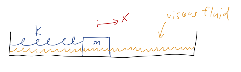
We’ll begin our study with the damped harmonic oscillator. Damping refers to energy loss, so the physical context of this example is a spring with some additional non-conservative force acting. Specifically, what people usually call “the damped harmonic oscillator” has a force which is linear in the speed, giving rise to the equation m \ddot{x} = - b\dot{x} - kx. The new force is the familiar linear drag force, so we can imagine this to be the equation describing a mass on a spring which is sliding through a high-viscosity fluid, like molasses:
As Taylor observes, another very important instance of this equation is the LRC circuit, which contains an inductor, a resistor, and a capacitor in series. The differential equation for the charge in such a circuit is L\ddot{Q} + R\dot{Q} + \frac{Q}{C} = 0. Since this is not a circuits class I won’t dwell on this example, but I point it out for those of you who might be more familiar with circuit equations.
Let’s rearrange the equation of motion slightly and divide out by the mass, as we did for the SHO: \ddot{x} + 2\beta \dot{x} + \omega_0^2 x = 0 where \beta = \frac{b}{2m},\ \ \omega_0 = \sqrt{\frac{k}{m}}, using the conventional notation for this problem. The frequency \omega_0 is called the natural frequency; as we can see, it is the frequency at which the system would oscillate if we removed the damping term by setting b=0. The other constant \beta is called the damping constant, and it is proportional to the strength of the drag force. \beta has the same units as \omega_0, i.e. frequency or 1/time.
6.3.1 Solving 2nd-order linear ODEs using operators
Once again, we have a linear, second-order, homogeneous ODE, so we just need to find two independent solutions to put together. Unfortunately, it’s a little harder to guess what the solutions will be just by inspection this time. Taylor uses the first method most physicists will reach for - guess and check, here guessing a complex exponential form. This sort of works, but in the special case \beta = \omega_0 (which we do want to cover) guess and check is much harder to use.
There is a more systematic way to find the answer, using the language of linear operators (as covered in Boas 8.5.) First of all, an operator is a generalized version of a function: it’s a map that takes an input to an output based on some specific rules. The derivative d/dt can be thought of as an operator, which takes an input function and gives us back an output function. The “linear” part refers to operators that follow two simple rules:
\frac{d}{dt} (f(t) + g(t)) = \frac{df}{dt} + \frac{dg}{dt}
\frac{d}{dt} (a f(t)) = a \frac{df}{dt}
We already know that these are both true for d/dt. What this means is that we can do algebra on the derivative operator itself. For example, using these properties we can write \frac{d^2f}{dt^2} + 3\frac{df}{dt} = 0 \Rightarrow \frac{d}{dt} \left( \frac{d}{dt} + 3 \right) f(t) = 0 or adopting the useful shorthand that D \equiv d/dt, D (D+3) f(t) = 0 = (D+3) D f(t).
On the last line, I re-ordered the two derivative terms. But this reordering is very useful, because it shows that there are two ways to satisfy the equation: both D f(t) = 0 and (D+3) f(t) = 0 will lead to solutions to the differential equation. Even better, the two solutions we get will be linearly independent (I won’t prove this, see Boas), which means that solving each of these simple first-order equations immediately gives us the general solution to the original equation!
This gives us a very useful method to solve a whole class of second-order linear ODEs:
Rewrite the ODE in the form (aD^2 + bD + c) f = 0.
Solve for the roots of the auxiliary equation, (aD^2 + bD + c) = 0 = (D - r_1) (D - r_2)
Obtain the general solution from the solutions of (D-r_1) f = 0 and (D - r_2) f = 0.
Here I’ve assumed a homogeneous ODE, i.e. the right-hand side is zero. We can use the same method for non-homogeneous equations, but there’s an extra step in that case: we have to add a particular solution, as we saw in the first-order case. Also, it’s very important above that the constants are constant - in other words, if D = d/dt, then a,b,c must all be independent of t or else the reordering trick doesn’t work (it’s easy to see that, for example, D (D+t) is not equal to (D+t) D.)
Now let’s use this method on the damped harmonic oscillator. Our ODE looks like \ddot{x} + 2\beta \dot{x} + \omega_0^2 x = 0 which we can rewrite as (D^2 + 2\beta D + \omega_0^2) x(t) = 0. To find the roots of the auxiliary equation, we can just use the quadratic formula: r_{\pm} = -\beta \pm \sqrt{\beta^2 - \omega_0^2}. The individual solutions, then, solve the first-order equations (D - r_{\pm}) x = 0, which we recognize as simple exponential solutions, x(t) \propto e^{r_{\pm} t}.
Thus, our general solution is: x(t) = C_1 e^{r_+ t} + C_2 e^{r_- t} \\ = C_1 e^{-\beta t + \sqrt{\beta^2 - \omega_0^2} t} + C_2 e^{-\beta t - \sqrt{\beta^2 - \omega_0^2} t} \\ = e^{-\beta t} \left( C_1 e^{\sqrt{\beta^2 - \omega_0^2} t} + C_2 e^{-\sqrt{\beta^2 - \omega_0^2}t} \right). (There is one subtlety here: if r_+ = r_-, then we have actually only found one solution. I’ll return to this case a little later.)
If we plug in \beta = 0 as a check, then we get \sqrt{-\omega_0^2} t = i\omega_0 t inside both of the exponentials in the second factor, giving back our undamped SHO solution as it should.
It should be obvious from looking at this that the relative size of \beta and \omega_0 will be very important in the qualitative behavior of these solutions: the exponentials inside the parentheses can be either real or imaginary as we change \beta relative to \omega_0. Let’s go through the possibilities.
6.3.2 Underdamped motion
Since we already know what happens at \beta = 0, let’s start with small \beta and turn the strength of the force up from there. (\beta is dimensionless, so by “small \beta” I of course mean “small \beta/\omega_0.”) In particular, as long as \beta < \omega_0, the combination \beta^2 - \omega_0^2 under the roots will always be negative. We define a new frequency \omega as follows: \sqrt{\beta^2 - \omega_0^2} = i \sqrt{\omega_0^2 - \beta^2} = i \omega_1. Why \omega_1? I am not sure, other than 1 is the number after 0! But I’ll stick with this notation because it’s what Taylor uses, and because we have to call this something other than \omega_0 (which we are already using) and \omega (which we will need for something else shortly.)
With this definition, we have for the overall solution x(t) = e^{-\beta t} \left(C_1 e^{i\omega_1 t} + C_2 e^{-i\omega_1 t} \right), or doing the same trick to combine the trig functions as before, x(t) = Ae^{-\beta t} \cos (\omega_1 t - \delta). So we once again have an oscillating solution, almost the same as the SHO, except the amplitude dies off exponentially as e^{-\beta t}. If we plot this, we can imagine an exponential “envelope” given by \pm Ae^{-\beta t}, with the actual solution oscillating back and forth between the sides of the envelope:
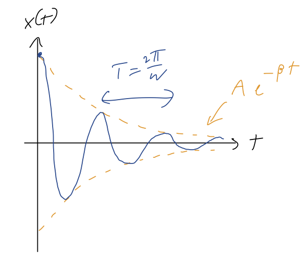
The solution above corresponds to releasing the oscillator at rest from some initial displacement. Note that this is no longer periodic, but the distance between maxima or minima within the envelope is still \tau = 2\pi / \omega_1. If \beta \ll \omega_0, then we notice that \omega_1 \approx \omega_0, so for very small damping the oscillation frequency is roughly the same as the natural oscillation. As the damping increases, the frequency of oscillation decreases (the peaks get further apart.)
By the way, notice what happens if we impose initial conditions on our simple harmonic oscillator solution: x(0) = A \cos(-\delta) \\ \dot{x}(0) = -A (\beta \cos (-\delta) + \omega_1 \sin(-\delta)) We can see right away that this is going to be trickier than the regular SHO solution; in particular, it is not true that \delta = 0 gives us the solution starting from rest here! Using some trig identities, this leads to the set of equations x(0) = A \cos \delta \\ \dot{x}(0) = -A \beta \cos \delta \left[1 - \frac{\omega_1}{\beta} \tan \delta \right]. This gets messy to solve, but for the specific case of starting from rest, \dot{x}(0) = 0 leads us to the simpler result 1 - \frac{\omega_1}{\beta} \tan \delta = 0 \Rightarrow \delta = \tan^{-1} \left( \frac{\omega_1}{\beta} \right) = \tan^{-1} \left( \frac{\sqrt{\omega_0^2 - \beta^2}}{\beta} \right) which we can plug in to for the phase shift, and then plug in to the first equation to find A. I won’t go further with this - you’d want to do it numerically for a given oscillator, the general case isn’t very enlightening. But I wanted to point out that A and \delta don’t have quite the same simple interpretations anymore for the damped oscillator.
6.3.3 Overdamped motion
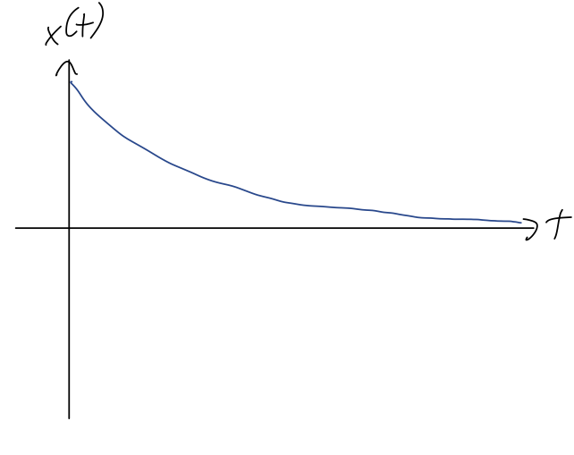
Let’s move on to the case where \beta > \omega_0 - exact equality is tricky, so we’ll do that last. In this case, all of the exponentials stay real, and we have x(t) = C_1 e^{-(\beta - \sqrt{\beta^2 - \omega_0^2}) t} + C_2 e^{-(\beta + \sqrt{\beta^2 - \omega_0^2}) t}. Since \sqrt{\beta^2 - \omega_0^2} < \beta given our assumptions, both terms decay exponentially in time, and there’s no oscillation at all. Here’s a sketch of this solution:
It’s instructive to factor out the first exponential term completely from our solution: x(t) = e^{-(\beta - \sqrt{\beta^2 - \omega_0^2}) t} \left( C_1 + C_2 e^{-2\sqrt{\beta^2 - \omega_0^2} t}\right). As t increases, the second term here is negligible for the long-term behavior of the system, unless we have C_1 = 0. Let’s match initial conditions to see what that would require: x_0 = x(0) = C_1 + C_2 \\ v_0 = \dot{x}(0) = -(\beta - \sqrt{\beta^2 - \omega_0^2}) C_1 - (\beta + \sqrt{\beta^2 - \omega_0^2}) C_2 We can solve this for C_1 = 0, and a bit of algebra reveals that it requires a specific relationship between v_0 and x_0, \frac{v_0}{x_0} = -(\beta + \sqrt{\beta^2 - \omega_0^2}). In particular, the minus sign tells us that this is only possible if v_0 and x_0 are in opposite directions. Aside from this rather special case, we can in general ignore the C_2 term completely at large t, finding that x(t) \rightarrow C_1 e^{-\alpha t} defining the decay parameter \alpha as the coefficient in the exponential decay of the max amplitude at large t, in this case \alpha = \beta - \sqrt{\beta^2 - \omega_0^2}. This solution exhibits some rather counterintuitive behavior: as we increase the strength of the damping force \beta, the decay parameter \alpha actually becomes smaller, approaching \alpha = 0 as \beta \rightarrow \infty! To make sense of this, let’s remember that the net force on our oscillator is F_{\textrm{net}} = F_{\textrm{drag}} + F_{\textrm{spring}} = -2m\beta \dot{x} - k x Both forces push our object back towards the origin. But if \beta is extremely large, then there is an enormous force even if we try to move at a relatively small speed, so it will take much longer in time for us to actually get to the origin. We still get there eventually, because the -kx spring force always keeps pulling us to the origin as long as x is non-zero.
6.3.4 Critical damping
Finally, we come back to the third possibility, which is \beta = \omega_0. If we go back to our original solution, this gives us x(t) = C_1 e^{-(\beta - \sqrt{\beta^2 - \omega_0^2}) t} + C_2 e^{-(\beta + \sqrt{\beta^2 - \omega_0^2}) t} \rightarrow C_1 e^{-\beta t} + C_2 e^{-\beta t}. Now we only have one solution, repeated twice! This means our solution is suddenly incomplete: we need two independent functions to add together to have a general solution. To find a second solution, since this is clearly a special case, let’s go back to the original differential equation and see what happens if \beta = \omega_0: \ddot{x} + 2 \beta \dot{x} + \beta^2 x = 0 Clearly e^{-\beta t} indeed works as a solution. To see the other one, let’s go back to our linear operator language and notice that the auxiliary equation in this case is easy to factorize: \left( \frac{d^2}{dt^2} + 2\beta \frac{d}{dt} + \beta^2 \right) x(t) = 0 becomes \left( D + \beta \right) \left( D + \beta \right) x(t) = 0. One way that this equation can be satisfied is just if \left( D + \beta \right) x(t) = 0, which matches on to our solution e^{-\beta t}. But the other possibility is that this combination isn’t zero: let’s call it \left( D + \beta \right) x(t) = u(t) \neq 0. Then we’re left with another first-order ODE, \left( D + \beta \right) u(t) = 0. So u(t) = C e^{-\beta t}, but now we have to work backwards a bit: \left( D + \beta \right) x(t) = C e^{-\beta t} We can use the general first-order solution in Boas to find the answer directly, but if you stare at this for a minute, you might think to try the following combination: if x(t) = C t e^{-\beta t} then \frac{dx}{dt} = C e^{-\beta t} - \beta C t e^{-\beta t} so the te^{-\beta t} will cancel out, matching the right-hand side. Thus, the general solution in this special case where \beta = \omega_0 is x(t) = C_1 e^{-\beta t} + C_2 t e^{-\beta t}. Once again, we see no oscillations - everything is pure exponential decay, but with an extra factor of t that only matters at small times. Once again as t becomes very large, the amplitude decays exponentially proportional to \beta.
6.3.5 Damped oscillator summary
Let’s summarize all of our solutions:
If \beta < \omega_0, the system is said to be underdamped. Our solution takes the form x(t) = Ae^{-\beta t} \cos (\omega_1 t - \delta), with oscillations at angular frequency \omega_1 = \sqrt{\omega_0^2 - \beta^2}, and the overall amplitude decaying with decay parameter \alpha = \beta.
If \beta = \omega_0, the system is critically damped. We have the funny solution we just found, x(t) = C_1 e^{-\beta t} + C_2 t e^{-\beta t}, with no oscillations and again the ampltiude at large times decaying exponentially with \alpha = \beta.
Finally, if \beta > \omega_0, the system is overdamped. In this case the general solution looks like x(t) = C_1 e^{-(\beta - \sqrt{\beta^2 - \omega_0^2}) t} + C_2 e^{-(\beta + \sqrt{\beta^2 - \omega_0^2}) t}. again pure exponential decay, but this time with decay parameter \alpha = \beta - \sqrt{\beta^2 - \omega_0^2}, which goes to zero as \beta gets larger and larger.
We can sketch the size of the decay parameter vs. the damping parameter \beta:
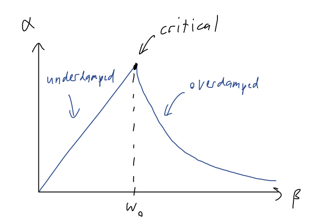
When designing a system that behaves like a damped oscillator, this tells us that it’s actually optimal to tune \beta (or \omega_0) so that the system is as close to critical as possible. A good example is shock absorbers in a car, which are designed to damp out the oscillations transferred from the road to the passengers.
6.3.6 Visualization using phase space
Let’s jump back for a moment to the simple harmonic oscillator (\beta = 0.) Given any solution for the position x(t), we also know the speed \dot{x}(t) of our oscillator at any given time. For example, using the phase-shift version of the solution: x(t) = A \cos (\omega t - \delta) \\ \Rightarrow \dot{x}(t) = -\omega A \sin (\omega t - \delta). Since we have a sine and a cosine, this is strongly reminiscent of polar coordinates with \phi = \omega t. In fact, we can make a nice plot by picking “coordinates” with \omega x on one axis and \dot{x} on the other:

This fictitious space, mixing position and speed with each other, is known as phase space. (Some references will just use x and \dot{x} as the axes, instead of \omega x and \dot{x}; since this is a fictitious space that we made up, the dimensions don’t have to match. But I’m going to keep the version with the \omega since it will simplify things a bit below.)
If we take a snapshot of our harmonic oscillator at any given moment t, recording x and \dot{x}, we obtain a single point in phase space. Letting t evolve for a given system then traces out a curve known as a phase portrait. Phase portraits are a useful way to visualize the behavior of a physical system.
Here, you should complete Tutorial 5D on “Phase space and harmonic motion”. (Tutorials are not included with these lecture notes; if you’re in the class, you will find them on Canvas.)
It’s useful to recall that the total energy of our harmonic oscillator is E = \frac{1}{2} m\dot{x}^2 + \frac{1}{2} kx^2 \\ = \frac{m}{2} \left( \dot{x}^2 + \omega^2 x^2 \right) using \omega^2 = k/m. This is just the equation of a circle in phase space the way we have defined the axes, with radius \sqrt{2E/m}. So another way to derive the “circular” motion in phase space is just that total energy E is constant for the simple harmonic oscillator!
As a comment: although I am starting with \omega x on the horizontal axis, this choice does have some drawbacks. For example, we can’t compare the phase portraits of two different oscillators easily, because we can only rescale by one frequency \omega. For more general applications of phase space, it is often better to just keep the axes as x vs. \dot{x}, in which case the energy conservation equation is written in the same way but interpreted slightly differently: 1 = \frac{x^2}{(2E/k)} + \frac{\dot{x}^2}{(2E/m)}. This is the equation of an ellipse, (x/a)^2 + (y/b)^2 = 1; the lengths of the semi-major axes are a=\sqrt{2E/k} and b=\sqrt{2E/m} = \omega \sqrt{2E/k} = \omega a.
Let’s continue on to the damped case. Since the phase-space orbit of the SHO is a circle (or ellipse, more generally) due to energy conservation, we expect that damping will drive our system towards the origin of phase space, (x, \dot{x}) = (0,0), as energy is removed and it comes to a stop. Starting with the underdamped case and taking a derivative, the speed is \dot{x}(t) = -\beta A e^{-\beta t} \cos (\omega_1 t - \delta) - \omega_1 A e^{-\beta t} \sin (\omega_1 t - \delta) or making the variable definition \phi = \omega_1 t - \delta, x(t) = Ae^{-\beta t} \cos \phi \\ \dot{x}(t) = -Ae^{-\beta t} (\beta \cos \phi + \omega_1 \sin \phi) This is already in a form that we can plug in to Mathematica to make a parametric plot using \phi, in order to visualize the phase-space trajectory (remember to substitute out t = (\phi + \delta) / \omega_1.) To go a little further by hand, let’s consider the case of small damping, \beta \ll \omega_0 (and thus \omega_1 \approx \omega_0). Then we can neglect the \cos \phi term in the speed, and we have simply: \omega_0 x(t) = \omega_0 Ae^{-\beta t} \cos \phi \\ \dot{x}(t) = -\omega_0 Ae^{\beta t} \sin \phi This is just the parametric equation for a circle, x = \rho \cos \phi and y = -\rho \sin \phi, except that the radius is decreasing exponentially as e^{-\beta t} instead of constant! So the phase portrait in this case, sketching \omega_0 x vs. \dot{x}, will look like a spiral:

Increasing the damping \beta will distort the spiral a bit as the term we neglected becomes important, but the qualitative motion is still the same. This also makes sense with conservation of energy; we recall that the distance to the origin in phase space is equal to the total energy of the oscillator. That’s still true here - but with the damping term, the total energy is falling to zero as our system evolves in time.
We could also do phase-space visualizations for the overdamped and critically damped cases. However, like the plots of x(t) in those cases, they’re not very interesting visually; the system is just pushed from its initial conditions directly towards the origin. (In general, as we increase \beta the spiraling behavior in the underdamped case will get faster, and there will be less spirals around the origin. Moving into overdamping is just the limit in which there are no spirals left - the phase space path never makes a complete circuit around by 2\pi.)