14 Addition of angular momentum
Despite their important differences, the spin and orbital angular momentum operators are fundamentally describing the same thing: what happens to our physical system under spatial rotations. Again, an analogy to classical mechanics is helpful: if we have a rigid rod at some position (x,y,z) in space, then spatial rotations will affect both the position of the rod, as well as its orientation (what direction the vector along the rod’s axis is pointing.)
In quantum mechanics, similarly, rotations will affect both spin and orbital angular momentum in the ways we have described thus far. However, this simultaneous rotation acts on two very different spaces: the infinite-dimensional position state, and the finite-dimensional space of spin states. We have a physical sense that these two spaces should be distinct in some sense, unless there is some interaction that couples them; the motion of the particle moving freely through space shouldn’t care whether it is internally spin-up or spin-down.
14.1 Quantum systems with orbital angular momentum and spin
We’ll use the formerly introduced notion of a direct product to describe this system, dividing the Hilbert space into position times spin, with eigenkets \ket{\vec{x}} \otimes \ket{s}. When we act with rotation by \phi around some axis \vec{n}, we can write the operator on the product space as \hat{\mathcal{D}}(R) = \exp \left( \frac{-i (\hat{\vec{L}} \cdot \vec{n}) \phi}{\hbar} \right) \otimes \exp \left( \frac{-i (\hat{\vec{S}} \cdot \vec{n}) \phi}{\hbar} \right).
This is nothing more than writing down how we already know rotations work on orbital angular momentum and on spin. Now, we can write this more compactly by defining a total angular momentum operator, which combines the angular momentum operators acting on the spin and orbital parts, as \hat{\vec{J}} = \hat{\vec{L}} \otimes \hat{1} + \hat{1} \otimes \hat{\vec{S}}. For simplicity, we’ll usually assume we know how to separate the subspaces and just write \hat{\vec{J}} = \hat{\vec{L}} + \hat{\vec{S}}; but for the first part of this discussion, I’m going to be careful and explicit with the product notation. If we write the total rotation operator in terms of \hat{\vec{J}}, it will just split back apart and we recover the same rotation matrix that \hat{\mathcal{D}}(R) we wrote above.
Why should we combine the two angular momentum operators like this? The answer comes from considering when rotations will be a good symmetry of the system - which, in quantum mechanics, is true when they preserve the Hamiltonian. A rotationally invariant \hat{H} satisfies \hat{\mathcal{D}}(R) \hat{H} \hat{\mathcal{D}}^{-1}(R) = \hat{H}. One way this can be satisfied is in a system that conserves both spin and orbital angular momentum separately, so [\hat{H}, \hat{\vec{L}}] = [\hat{H}, \hat{\vec{S}}] = 0. But it’s also possible, and even common, to find systems (like the hydrogen atom!) where only the total angular momentum is conserved, [\hat{H}, \hat{\vec{J}}] = 0, but \hat{\vec{L}} and \hat{\vec{S}} are not conserved on their own.
To understand how this works, let’s start by putting some of our math notation on firmer ground; we need a better understanding of how to put smaller Hilbert spaces together to form a larger space.
14.1.1 Direct sums and tensor products
I’m going to do a little mini-review here: if you’re still puzzled by what we’re doing, you should have a look at these nice lecture notes from Hitoshi Murayama about tensor products.
Suppose we have two vector spaces V_A and V_B, with dimensions m and n. They each have a set of basis vectors \{\hat{e}_1, ..., \hat{e}_m\} and \{\hat{f}_1, ..., \hat{f}_n\}. Suppose we want to combine them together to form a single vector space: how can we do it?
One possibility is to form the direct sum, V_A \oplus V_B. This creates a new (m+n)-dimensional vector space with basis simply equal to the union of the two original bases, i.e. \{\hat{e}_1, ..., \hat{e}_m, \hat{f}_1, ... \hat{f}_n \}. If \vec{v} is a vector in V_A and \vec{w} a vector in V_B, we can also define the vector direct sum v \oplus w in the obvious way: its m + n components are just given by stacking the components in each individual space. For example, if m=2 and n=3, then \vec{v} \oplus \vec{w} = \left( \begin{array}{c} v_1 \\ v_2 \\ w_1 \\ w_2 \\ w_3 \end{array} \right).
All of our original vectors are in the new direct-sum space, e.g. for every \vec{v} in V_A, we can write \vec{v} \oplus \vec{0} in V_A \oplus V_B.
If A is a matrix acting on vectors in V_A and B is a matrix acting on V_B, then we can combine them block-diagonally to obtain a matrix acting on V_A \oplus V_B: A \oplus B = \left( \begin{array}{cc} A_{m \times m} & 0_{m \times n} \\ 0_{n \times m} & B_{n \times n} \end{array} \right). This doesn’t imply that every matrix on the direct sum space can be written in this block-diagonal form, but we can make such a matrix from any matrices on the original spaces. When working with such composite matrices, the operations are very simple: we see that (A_1 \oplus B_1) (A_2 \oplus B_2) = (A_1 A_2) \oplus (B_1 B_2) \\ (A \oplus B) (\vec{v} \oplus \vec{w}) = (A\vec{v}) \oplus (B\vec{w}) i.e. all the operations just break apart into operations on our original spaces. This also applies to commutators: from above, we immediately have [(A_1 \oplus B_1), (A_2 \oplus B_2)] = [A_1, A_2] \oplus [B_1, B_2].
The other way we can form a new vector space from our original pair is by taking the direct product, V_A \otimes V_B (also known as the “tensor product”.) In the direct product, we define our new basis vectors by pairing together all possible combinations of the original basis, i.e. \{\hat{e}_i \otimes \hat{f}_j\},\ \ i = 1...m,\ \ j=1...n This gives a space of dimension mn. The “tensor” in the name is self-evident, since our basis vectors are now tensors - you can think of them as having two indices, i and j.
Let’s go back to our concrete example from above where m=2 and n=3. Now our direct product basis is six-dimensional: given two vectors \vec{v} and \vec{w}, their tensor product is \vec{v} \otimes \vec{w} = \left( \begin{array}{c} v_1 w_1 \\ v_1 w_2 \\ v_1 w_3 \\ v_2 w_1 \\ v_2 w_2 \\ v_2 w_3 \end{array} \right). For matrices, we can similarly form A \otimes B, but it’s not as simple as just stacking them together anymore. We define the direct product of matrices by requiring that its action on direct products of vectors decomposes over the original spaces, i.e. (A \otimes B) (\vec{v} \otimes \vec{w}) = (A\vec{v} \otimes B\vec{w}). The resulting matrix (which you may also hear referred to as the matrix outer product or Kronecker product) will usually be rather dense. It’s easiest to see how this works if one of the matrices is the identity, e.g. A \otimes I = \left( \begin{array}{cccccc} a_{11} & 0 & 0 & a_{12} & 0 & 0 \\ 0 & a_{11} & 0 & 0 & a_{12} & 0 \\ 0 & 0 & a_{11} & 0 & 0 & a_{12} \\ a_{21} & 0 & 0 & a_{22} & 0 & 0 \\ 0 & a_{21} & 0 & 0 & a_{22} & 0 \\ 0 & 0 & a_{21} & 0 & 0 & a_{22} \end{array} \right) You can verify that multiplying this out gives the expected result (A \otimes I) (\vec{v} \otimes \vec{w}) = (A\vec{v}) \otimes \vec{w}.
So in general, direct products are much more complicated to work with than direct sums; most natural matrices we build from individual spaces are not diagonal. On the other hand, direct sums give block diagonal subspaces that can easily be worked with separately.
Although the details are more complicated, the direct product still satisfies the important property that products of matrices break apart as expected: (A \otimes B) (C \otimes D) = (AC) \otimes (BD). Addition satisfies a distribution property, A \otimes B + A \otimes D = A \otimes (B+D) \\ A \otimes B + C \otimes B = (A + C) \otimes B, and scalar multiplication also works as you would expect, (cA) \otimes B = A \otimes (cB) = c(A \otimes B).
All of the above lets us write down a nice little identity for commutators of direct-product operators:
[(A_1 \otimes B_1), (A_2 \otimes B_2)] = \frac{1}{2} [\hat{A}_1, \hat{A}_2] \otimes \{\hat{B}_1, \hat{B}_2\} + \frac{1}{2} \{\hat{A}_1, \hat{A}_2\} \otimes [\hat{B}_1, \hat{B}_2].
(There’s a similar identity for anti-commutators, which you can find in the exercise below.)
Prove the identity above, using the given properties of direct products.
Answer:
We start with the identity we previously found for regular operators, \hat{A} \hat{B} = \frac{1}{2} \left( [\hat{A}, \hat{B}] + \{\hat{A}, \hat{B}\} \right) then we see that (\hat{A}_1 \hat{A}_2) \otimes \hat{B} = \frac{1}{2} [\hat{A}_1, \hat{A}_2] \otimes \hat{B} + \frac{1}{2} \{\hat{A}_1, \hat{A}_2\} \otimes \hat{B}
Let’s see what this implies for a commutator: [(A_1 \otimes B_1), (A_2 \otimes B_2)] = (A_1 \otimes B_1) (A_2 \otimes B_2) - (A_2 \otimes B_2) (A_1 \otimes B_1) \\ = (A_1 A_2 \otimes B_1 B_2) - (A_2 A_1 \otimes B_2 B_1) The first term can be broken into four pieces: A_1 A_2 \otimes B_1 B_2 = \frac{1}{2} [\hat{A}_1, \hat{A}_2] \otimes B_1 B_2 + \frac{1}{2} \{\hat{A}_1, \hat{A}_2\} \otimes B_1 B_2 \\ = \frac{1}{4} \left( [\hat{A}_1, \hat{A}_2] \otimes [\hat{B}_1, \hat{B}_2] + [\hat{A}_1, \hat{A}_2] \otimes \{\hat{B}_1, \hat{B}_2 \} \right. \\ \left. + \{\hat{A}_1, \hat{A}_2\} \otimes [\hat{B}_1, \hat{B}_2] + \{\hat{A}_1, \hat{A}_2\} \otimes \{\hat{B}_1, \hat{B}_2 \} \right) Back to the commutator, the second term is the same but with labels 1 and 2 swapped. This means that any term which is symmetric under 1 \leftrightarrow 2 will just cancel, while antisymmetric terms will add. As a result, we find the formula: [(A_1 \otimes B_1), (A_2 \otimes B_2)] = \frac{1}{2} [\hat{A}_1, \hat{A}_2] \otimes \{\hat{B}_1, \hat{B}_2\} + \frac{1}{2} \{\hat{A}_1, \hat{A}_2\} \otimes [\hat{B}_1, \hat{B}_2]. Since we relied on antisymmetry here, we can easily read off a corollary formula that we won’t need right away, but that might be useful someday: \{(A_1 \otimes B_1), (A_2 \otimes B_2) \} = \frac{1}{2} [\hat{A}_1, \hat{A}_2] \otimes [\hat{B}_1, \hat{B}_2] + \frac{1}{2} \{\hat{A}_1, \hat{A}_2\} \otimes \{\hat{B}_1, \hat{B}_2 \}.Now we have the tools to understand how Hamiltonians can conserve only total \hat{\vec{J}} but not the individual components \hat{\vec{L}} and \hat{\vec{S}}. Since we’re considering a Hilbert space consisting of a direct product of position and spin \ket{\vec{x}} \otimes \ket{s}, one possibility is that the Hamiltonian can likewise be written in terms of \hat{\vec{L}} and \hat{\vec{S}} operators, meaning that it breaks apart: \hat{H} = \hat{H}_L \otimes \hat{H}_S. Rotational invariance means that [\hat{H}, \hat{J}] = 0, as we discussed above. Now we can use our commutator identity: 0 = [\hat{H}, \hat{\vec{J}}] = [\hat{H}_L \otimes \hat{H}_S, \hat{\vec{L}} \otimes \hat{1} + \hat{1} \otimes \hat{\vec{S}}] \\ = \frac{1}{2} [\hat{H}_L, \hat{\vec{L}}] \otimes \{\hat{H}_S, \hat{1}\} + \frac{1}{2} \{\hat{H}_L, \hat{1}\} \otimes [\hat{H}_S, \hat{\vec{S}}] where I’ve discarded two other terms that contain a commutator with \hat{1} that vanishes. This will be zero as long as both individual angular momenta are conserved, i.e. if [\hat{H}_L, \hat{\vec{L}}] = [\hat{H}_S, \hat{\vec{S}}] = 0 then the whole thing is invariant under rotations and \hat{\vec{J}} is conserved too, trivially.
Having written things out in this way, we can see that the condition of commuting with both pieces of \hat{\vec{J}} doesn’t have to be true in reverse, since the other possibility is that the two terms cancel each other: [\hat{H}_L, \hat{\vec{L}}] \otimes \hat{H}_S = -\hat{H}_L \otimes [\hat{H}_S, \hat{\vec{S}}].
This, however, is a curiosity as far as I can tell: I don’t know of any concrete Hamiltonians that satisfy the condition above without both sides just being zero. It seems difficult to achieve without just breaking Lorentz invariance explicitly, but maybe one of you will find it useful someday…or maybe you can prove that this doesn’t lead anywhere useful.
The other possibility, which is in fact very common, is that we have a Hamiltonian that doesn’t split apart nicely into components as above. In the present case, it will fail to split in the presence of a spin-orbit coupling term, usually written as \hat{\vec{L}} \cdot \hat{\vec{S}}. Being more careful about the direct-product notation, we know that this should really be written as (\hat{\vec{L}} \otimes \hat{1}) \cdot (\hat{1} \otimes \hat{\vec{S}}) = \hat{\vec{L}} \otimes \hat{\vec{S}} = \hat{L}_x \otimes \hat{S}_x + \hat{L}_y \otimes \hat{S}_y + \hat{L}_z \otimes \hat{S}_z. This, plainly, can’t be separated into \hat{H}_L \otimes \hat{H}_S, since the dot product joins the two together.
Why should such a term exist in our Hamiltonian? Since spins of charged particles act as magnetic moments, a spin-orbit term can be derived for hydrogen as an interaction of the electron’s spin with the electric field of the proton. More generally, we can argue in the other direction: while we know that rotational invariance should be a good symmetry of our Hamiltonian, there’s no reason it has to hold for individual parts of the Hamiltonian - that is, the statement “the world is invariant under rotations” only requires [\hat{H}, \hat{\vec{J}}] = 0, so symmetry gives us no reason to expect there won’t be a spin-orbit term. (I like the succinct way that David Tong puts this in his quantum notes, paraphrased: “there is no law of conservation of spin.”)
14.2 Addition of angular momentum
Let’s now go through a somewhat more general treatment for addition of angular momentum. This will cover the case above, relevant for atoms, but also common cases like having two spins coupled together.
Suppose we have a system with two angular momentum operators, \hat{\vec{J}}_1 and \hat{\vec{J}}_2, acting on different subspaces. Individually, these operators satisfy the usual commutation relations, [\hat{J}_{1i}, \hat{J}_{1j}] = i\hbar \epsilon_{ijk} \hat{J}_{1k}, and the same for the components of \hat{\vec{J}}_2. Since they act on different subspaces of our Hilbert space, the operators commute with each other on the joint Hilbert space: [\hat{J}_{1i}, \hat{J}_{2j}] = [\hat{J}_{1i} \otimes \hat{1}, \hat{1} \otimes \hat{J}_{2j}] = 0. An arbitrary rotation generated by these two angular momentum operators acts separately on the two subspaces, but with the same axis of rotation \vec{n} and same spatial angle \phi: \hat{\mathcal{D}}(R) = \hat{\mathcal{D}}_1(R) \otimes \hat{\mathcal{D}}_2(R) = \exp \left( \frac{-i (\hat{\vec{J}}_1 \cdot \vec{n}) \phi}{\hbar} \right) \otimes \exp \left( \frac{-i (\hat{\vec{J}}_2 \cdot \vec{n}) \phi}{\hbar} \right) Now, we can define a total angular-momentum operator, \hat{\vec{J}} = \hat{\vec{J}}_1 + \hat{\vec{J}}_2 where from here on I will stop writing out the direct products, and just implicitly keep track of how things act on different subspaces. (Strictly speaking, I should have written the above as \hat{\vec{J}} = \hat{\vec{J}}_1 \otimes \hat{1} + \hat{1} \otimes \hat{\vec{J}}_2, for example.) Because \hat{\vec{J}}_1 and \hat{\vec{J}}_2 independently satisfy the angular momentum commutation relations and they commute with each other, it’s easy to see that total \hat{\vec{J}} is also an angular momentum operator: [\hat{J}_i, \hat{J}_j] = i\hbar \epsilon_{ijk} \hat{J}_k This makes physical sense; by way of the rotation formula I wrote above, we can think of \hat{\vec{J}} as being the generator of rotations for both subspaces 1 and 2 at once.
What do the eigenkets of this combined system look like? We already know that for an individual angular momentum operator, we typically use \hat{\vec{J}}{}^2 and \hat{J}_z as a CSCO, labelling our eigenkets with their respective quantum numbers \ket{jm}. Clearly, one possible choice for this system is just to use this basis for both subspaces, i.e. we take the CSCO \textrm{CSCO 1:}\ \ \{ \hat{\vec{J}}_1{}^2, \hat{\vec{J}}_2{}^2, \hat{J}_{1,z}, \hat{J}_{2,z} \}, and the eigenkets are then labelled \ket{j_1 j_2; m_1 m_2}. This basis is known as the product basis, since the eigenkets are simply direct products of eigenkets for the individual angular momentum operators. This is always a valid way to label the angular-momentum eigenkets, but if the Hamiltonian contains the term \hat{\vec{J}}_1 \cdot \hat{\vec{J}}_2 (like the spin-orbit coupling for example), then we can’t include the Hamiltonian in this CSCO, and solving for the time-evolution will be complicated in this basis.
Can we find a second CSCO that can include more general Hamiltonians that have the operator \hat{\vec{J}}_1 \cdot \hat{\vec{J}}_2 in them? A useful starting point is to notice that this operator satisfies a nice identity: \hat{\vec{J}}{}^2 = (\hat{\vec{J}}_1 + \hat{\vec{J}}_2)^2 \\ = \hat{\vec{J}}_1{}^2 + \hat{\vec{J}}_2{}^2 + 2 \hat{\vec{J}}_1 \cdot \hat{\vec{J}}_2 \\ \Rightarrow \hat{\vec{J}}_1 \cdot \hat{\vec{J}}_2 = \frac{1}{2} \left( \hat{\vec{J}}{}^2 - \hat{\vec{J}}_1{}^2 - \hat{\vec{J}}_2{}^2 \right). This suggests starting with the three operators \hat{\vec{J}}{}^2, \hat{\vec{J}}_1{}^2, \hat{\vec{J}}_2{}^2 for our new CSCO; from this identity it’s easy to show they all commute with each other, and with the dot product \hat{\vec{J}}_1 \cdot \hat{\vec{J}}_2. We just need one more operator to get a complete set, since we had four operators in the other one; an obvious choice is \hat{J}_z, the z-component of the total angular momentum, which is easily verified to commute with all of the squared operators above. So we have our second CSCO: \textrm{CSCO 2:}\ \ \{ \hat{\vec{J}}{}^2, \hat{J}_z, \hat{\vec{J}}_1{}^2, \hat{\vec{J}}_2{}^2 \}. Using this different set of commuting operators amounts to a change of basis; in this basis, we label the eigenkets as \ket{j_1 j_2; j m}. The basis of eigenstates for CSCO 2 is generally known as the total angular momentum basis. Two of the labels are the same; we’ve traded m_1 and m_2 for j and m. To be explicit, the action of the operators in our second CSCO is given by: \hat{\vec{J}}_1{}^2 \ket{j_1 j_2; j m} = \hbar^2 j_1 (j_1+1) \ket{j_1 j_2; jm} \\ \hat{\vec{J}}_2{}^2 \ket{j_1 j_2; j m} = \hbar^2 j_2 (j_2 + 1) \ket{j_1 j_2; jm} \\ \hat{\vec{J}}{}^2 \ket{j_1 j_2; j m} = \hbar^2 j (j+1) \ket{j_1 j_2; jm} \\ \hat{J}_z \ket{j_1 j_2; j m} = \hbar m \ket{j_1 j_2; j m}. This is a much more useful basis for cases where the Hamiltonian contains dot products of angular momenta, by construction. More concretely, we can see the same thing is true after the fact by thinking about what \hat{\vec{J}}_1 \cdot \hat{\vec{J}}_2 looks like in both bases. In CSCO 2, the dot-product operator is diagonal by construction. On the other hand, in CSCO 1 we can derive the identity \hat{\vec{J}}_1 \cdot \hat{\vec{J}}_2 = \hat{J}_{1z} \hat{J}_{2z} + \frac{1}{2} (\hat{J}_{1+} \hat{J}_{2-} + \hat{J}_{1-} \hat{J}_{2+}). which is manifestly not diagonal, due to the presence of the ladder operators.
14.2.1 Eigenvalues in the total angular momentum basis
We can gain some useful insights by acting with particular combinations of operators. For example, we have the identity (\hat{J}_z - \hat{J}_{1z} - \hat{J}_{2z}) \ket{j_1 j_2; j m} = 0, which holds for any ket since the combination of operators here gives the null operator. If we multiply on the left with a state in the “product basis”, we have \bra{j_1 j_2; m_1 m_2} (\hat{J}_z - \hat{J}_{1z} - \hat{J}_{2z}) \ket{j_1 j_2; j m} \\ = (m - m_1 - m_2) \left\langle j_1 j_2; m_1 m_2 | j_1 j_2; j m \right\rangle = 0. Thus, the Clebsch-Gordan coefficients always vanish unless the eigenvalues satisfy the condition m = m_1 + m_2. A somewhat more difficult property to prove is the restriction on the eigenvalue j: |j_1 - j_2| \leq j \leq j_1 + j_2. If we think of \hat{\vec{J}} as a vector sum of the individual total angular momentum operators, then this makes perfect sense, but these are operators and not just normal vectors. The proof of this relation is recursive and not very enlightening, but it’s in appendix C of Sakurai if you’re interested.
While not a rigorous derivation, we can convince ourselves this has to be true just by counting up all of the eigenstates; we know that the dimension of our Hilbert space has to be the same when we change basis, so we should get the same answer. In the product basis, we know that there are (2j_i + 1) possible m_i eigenvalues, so the number of states is N = (2j_1 + 1)(2j_2 + 1). In the total angular momentum basis, we have (2j+1) states for each value of j allowed: N = \sum_{j=j_{min}}^{j_{max}} (2j+1) = j_{max} (j_{max} + 1) - j_{min} (j_{min} - 1) + (j_{max} - j_{min} + 1) \\ = (j_{max} + j_{min} + 1) (j_{max} - j_{min} + 1) which is clearly equal if we make the choices for j_{min} and j_{max} given above.
Before we go further with generalities, it’s useful to see the a simple (and useful!) example: the combination of spin and angular momentum for a spin-1/2 particle. We’ll follow aspect of this example through the rest of this chapter.
14.3 Example: energy splittings for 2p hydrogen
As our first application of this machinery, let’s study the energy levels of hydrogen for the 2p orbital (this is p-wave so l=1, and of course s=1/2). As I mentioned, the textbook solution for hydrogen solves only in terms of orbital angular momentum and ignores the spin of the electron. The first correction to consider is the spin-orbit coupling, \hat{H}_{so} = f(r) \hat{\vec{S}} \cdot \hat{\vec{L}}. where our two angular momentum operators are the electron spin, \hat{\vec{S}}, and its orbital angular momentum, \hat{\vec{L}}. You can look up what f(r) actually is in a textbook - it’s a combination of a bunch of constants and a 1/r^3 dependence - but for this example it doesn’t really matter for how we treat the spin-orbit interaction (except that it will reappear in an integral at the end.)
In principle, the spin-orbit coupling modifies the Schrödinger equation itself, so we’d have to (re-)solve the hydrogen atom at this point. But the spin-orbit coupling is rather small, so I will instead invoke a result from perturbation theory: we can approximate the energy shift by calculating the expectation value of the perturbation Hamiltonian in terms of the old eigenstates, E_{so} \approx \bra{j,m} \hat{H}_{so} \ket{j,m}. We’ll prove this result later on, but for now just take my word for it.
Since we’ve specified a p-wave orbital, we have l=1 and of course s=1/2. There are six possible states \ket{l, s; m_l, m_s} that we can write down in the product basis: \ket{1, \tfrac{1}{2}; 1, \tfrac{1}{2}},\ \ \ \ket{1, \tfrac{1}{2}; 1, -\tfrac{1}{2}}, \\ \ket{1, \tfrac{1}{2}; 0, \tfrac{1}{2}},\ \ \ \ket{1, \tfrac{1}{2}; 0, -\tfrac{1}{2}}, \\ \ket{1, \tfrac{1}{2}; -1, \tfrac{1}{2}},\ \ \ \ket{1, \tfrac{1}{2}; -1, -\tfrac{1}{2}}. Now, we can just apply the operator \hat{\vec{S}} \cdot \hat{\vec{L}} to these states directly; they’re not eigenstates of that operator (since it contains the x and y components of both angular momenta), but we know how to evaluate them. But since it isn’t diagonal (it contains ladder operators as noted above), it will be much simpler in the total angular momentum basis, since \hat{\vec{S}} \cdot \hat{\vec{L}} = (\hat{\vec{S}} + \hat{\vec{L}})^2 - \hat{\vec{S}}{}^2 - \hat{\vec{L}}{}^2 \\ = \frac{1}{2} (\hat{\vec{J}}{}^2 - \hat{\vec{L}}{}^2 - \hat{\vec{S}}{}^2). Let’s enumerate the six states in the new basis: the condition on j from above is 1/2 \leq j \leq 3/2, while we also have m = m_l + m_s. Since m_s is always a half-integer, m also has to be a half integer, which means j=1 won’t work. So the new basis states must be (just writing as \ket{j,m}): \ket{\tfrac{1}{2}, \tfrac{1}{2}},\ \ \ \ket{\tfrac{1}{2}, -\tfrac{1}{2}}, \\ \ket{\tfrac{3}{2}, \tfrac{3}{2}},\ \ \ \ket{\tfrac{3}{2}, -\tfrac{3}{2}}, \\ \ket{\tfrac{3}{2}, \tfrac{1}{2}},\ \ \ \ket{\tfrac{3}{2}, -\tfrac{1}{2}}. \\ Again, this is a change of basis, so the fact that we have the same number of basis states is a good check that we’ve done things correctly. Here I’m keeping the total angular momentum eigenvalues to label the product-basis states, but dropping them in the total basis states, which will help us keep track of which is which.
The action of the spin-orbit coupling on total angular momentum basis states is nice and simple: \hat{H}_{so} \ket{j, m} = \frac{1}{2} \hbar^2 f(r) (j(j+1) - l(l+1) - s(s+1)) \ket{j, m}. This depends only on j and not m, so we only have two distinct spin-orbit eigenvalues: \hat{H}_{so} \ket{\tfrac{1}{2}, m} = -\hbar^2 f(r) \ket{\tfrac{1}{2}, m}, \\ \hat{H}_{so} \ket{\tfrac{3}{2}, m} = \frac{1}{2} \hbar^2 f(r) \ket{\tfrac{3}{2}, m}.
There is still some radial dependence to deal with, but that means just have to average over the radial wavefunction as part of the expectation value: E_{so,j} = \int_0^\infty dr\ r^2 |R_{nl}(r)|^2 f(r)\ \bra{j, m} \hat{\vec{S}} \cdot \hat{\vec{L}} \ket{j,m}, where R_{nl}(r) are the standard radial wavefunctions for hydrogen. I’ll skip the actual details of this integral, but the result for 2p hydrogen turns out to be quite small, with the spin-orbit splitting on the order of 5 \times 10^{-5} eV. Even without the integral, we have obtained the qualitative result that the 2p energy level splits apart into two energy levels with j=1/2 and j=3/2; furthermore, the j=1/2 splitting is negative, so it is the lower energy level.
With the inclusion of orbital angular momentum, it’s no longer sufficient for us to use the ordinary spectroscopic notation (s,p,d,f,...) that we introduced before. For example, the spin-1/2 electron in an l=1 orbital has two distinct energy levels, corresponding to j=1/2 and j=3/2. To deal with systems containing combinations of spin and angular momentum, we introduce the modified spectroscopic notation, which looks like this: {}^{2S+1} L_J Here L is the orbital angular momentum quantum number, which we now write as a capital letter: l=0 becomes S, l=1 is P, and so on. S is the spin quantum number, so 2S+1 labels the number of degenerate spin states. The two states we have in the current example are thus {}^{2}P_{1/2} and {}^{2}P_{3/2}.
A state with no angular momentum and no spin would be {}^{1}S_0. This isn’t as trivial as it looks; in fact, such a spectroscopic label occurs very frequently in atoms with multiple electrons. The ground state of helium, and indeed of each of the noble gases, is labeled {}^{1}S_0.
If we consider this effect together with the 2s energy level (which has no spin-orbit term), we could sketch an energy splitting diagram like the following:
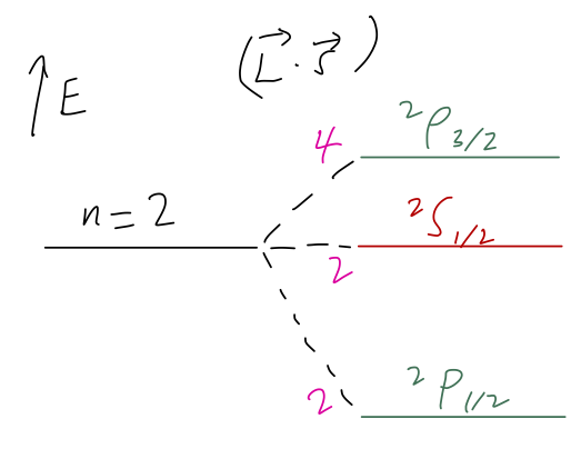
(Here I’ve labelled the degeneracy of each state in magenta along the splitting lines.) I should point out that this is qualitatively right, but for the wrong reasons; in the real world there are other effects in hydrogen of the same order of magnitude that contribute to the splittings between these three spectroscopic levels. We may see them in detail at the end of the semester. (Actually, the {}^2S_{1/2} state is much closer to the {}^2P_{1/2} state, due to some of these other effects.)
14.4 Clebsch-Gordan coefficients
Since the difference between our choices of CSCO is a change of basis, we know that we can write down a unitary transformation relating one basis to another, just by inserting a complete set of states: \ket{j_1 j_2; j m} = \sum_{m_1} \sum_{m_2} \ket{j_1 j_2; m_1 m_2} \left\langle j_1 j_2; m_1 m_2 | j_1 j_2; j m \right\rangle. The components of the transformation matrix, i.e. the inner products appearing above, are known as Clebsch-Gordan coefficients, and they are of enormous importance whenever we want to study systems with multiple angular momentum operators.
To motivate why Clebsch-Gordan coefficients are important, let’s continue with our example of 2p hydrogen. Suppose that we place our hydrogen atom in a very weak magnetic field. This gives rise to an additional perturbation on top of the spin-orbit coupling, of the following form:
\hat{H}_B = \mu_B B (\hat{L}_z + 2 \hat{S}_z).
This cannot be easily written in terms of the total angular momentum. If we have both this and the spin-orbit interaction, we need the Clebsch-Gordan coefficients to work in both bases at once.
Let’s begin working out the change of basis. To do so, I will demonstrate a general procedure for finding the C-G coefficients (although this is not an efficient procedure, especially for higher angular momentum; if you are dealing professionally with Clebsch-Gordan coefficients, you will probably use pre-calculated tables or computer packages.)
We begin “at the top”, with the state with maximum m, \ket{\tfrac{3}{2}, \tfrac{3}{2}}. Since there is only one product-basis state satisfying m_l + m_s = 3/2, the sum \ket{j_1 j_2; j m} = \sum_{m_1} \sum_{m_2} \ket{j_1 j_2; m_1 m_2} \left\langle j_1 j_2; m_1 m_2 | j_1 j_2; j m \right\rangle. has only one term: \ket{\tfrac{3}{2}, \tfrac{3}{2}} = \ket{1, \tfrac{1}{2}; 1, \tfrac{1}{2}} \left\langle 1, \tfrac{1}{2}; 1, \tfrac{1}{2} | \tfrac{3}{2},\tfrac{3}{2} \right\rangle. Since we assume the original state is already normalized, the Clebsch-Gordan coefficient appearing here must simply be 1.
Moving on to \ket{\tfrac{3}{2}, \tfrac{1}{2}}, there are two states in the original basis that will contribute, so we can’t make such a simple argument. However, since we already have one state in the new basis, we can just use the ladder operators to derive other states. The ladder operators in the total angular momentum basis are just \hat{J}_{\pm} = \hat{L}_{\pm} + \hat{S}_{\pm} This is a good time to remind ourselves that the ladder operators act like so: \hat{J}_{\pm} \ket{j, m} = \hbar \sqrt{(j \mp m) (j \pm m + 1)} \ket{j, m \pm 1}. Now, acting on the total-basis state, we have \hat{J}_- \ket{\tfrac{3}{2}, \tfrac{3}{2}} = \sqrt{3} \hbar \ket{\tfrac{3}{2}, \tfrac{1}{2}}. But from the definition above, we can also write \hat{J}_- \ket{\tfrac{3}{2}, \tfrac{3}{2}} = (\hat{L}_- + \hat{S}_-) \ket{1, \tfrac{1}{2}; 1, \tfrac{1}{2}} \\ = \hbar \sqrt{2} \ket{1,\tfrac{1}{2}; 0, \tfrac{1}{2}} + \hbar \ket{1, \tfrac{1}{2}; 1, -\tfrac{1}{2}}. \\ Thus, the total-basis state is given in terms of the product basis by \ket{\tfrac{3}{2}, \tfrac{1}{2}} = \sqrt{\frac{2}{3}} \ket{1, \tfrac{1}{2}; 0, \tfrac{1}{2}} + \sqrt{\frac{1}{3}} \ket{1, \tfrac{1}{2}; 1, -\tfrac{1}{2}}. As a check, we notice that this state is properly normalized, since the squared coefficients add to 1. To get \ket{\tfrac{3}{2}, -\tfrac{1}{2}}, we can just apply the lowering operator again, and then again to get \ket{\tfrac{3}{2}, -\tfrac{3}{2}}, but let me come back to those; there’s a nice symmetry-based way to get them instead of just grinding through ladder operators.
This leaves us with two states to find; the pair of j=1/2 states. They will each overlap with two of the product-basis states, so we don’t have a nice starting point for the use of ladder operators anymore. However, we can still use the ladder operators to make progress. If we try to raise the state \ket{\tfrac{1}{2}, \tfrac{1}{2}}, we know we should get zero, so: \hat{J}_+ \ket{\tfrac{1}{2}, \tfrac{1}{2}} = 0 = (\hat{L}_+ + \hat{S}_+) \left( \alpha \ket{1, \tfrac{1}{2}; 1, -\tfrac{1}{2}} + \beta \ket{1, \tfrac{1}{2}; 0, \tfrac{1}{2}} \right) \\ = \hbar \alpha \ket{1, \tfrac{1}{2}; 1, \tfrac{1}{2}} + \sqrt{2} \hbar \beta \ket{1, \tfrac{1}{2}; 1, \tfrac{1}{2}}. So \alpha + \sqrt{2} \beta = 0, and the state must also be properly normalized, so \alpha^2 + \beta^2 = 1. This is all we need to solve for the coefficients: we can rewrite the first equation in the form \alpha^2 - 2\beta^2 = 0, and then the solution is easy: \ket{\tfrac{1}{2}, \tfrac{1}{2}} = \sqrt{\frac{2}{3}} \ket{1, \tfrac{1}{2}; 1, -\tfrac{1}{2}} - \sqrt{\frac{1}{3}} \ket{1, \tfrac{1}{2}; 0, \tfrac{1}{2}}. Note that the sign ensures that this state is orthogonal to the similar-looking \ket{\tfrac{3}{2}, \tfrac{1}{2}} state; in fact, we could have solved for these coefficients just by requiring orthogonality in this case. The last state \ket{\tfrac{1}{2}, -\tfrac{1}{2}} can then be found using the lowering operator on \ket{\tfrac{1}{2}, \tfrac{1}{2}} once more.
Note that there is an overall sign ambiguity above; we could have instead chosen \alpha to be negative and \beta positive. This is secretly present even before we get to this point; even insisting that our Clebsch-Gordan coefficients all be real, we could have taken (-1) instead of (+1) times the product-basis states for the m=\pm 3/2 states. The standard sign convention for the C-G coefficients, and the one we will follow, is that the overlap between the highest components of \hat{\vec{J}}_1 and \hat{\vec{J}} is always positive, i.e. \left\langle j_1 j_2; j j | j_1 j_2; j_1 m_2 \right\rangle > 0. In our 2p hydrogen example, this gives the conditions \left\langle \tfrac{3}{2}, \tfrac{3}{2} | 1, \tfrac{1}{2}; 1, \tfrac{1}{2} \right\rangle > 0,\\ \left\langle \tfrac{1}{2},\tfrac{1}{2} | 1, \tfrac{1}{2}; 1, -\tfrac{1}{2} \right\rangle > 0.
From here, applying lowering operators as we did above fixes the signs of all of the other states - and, incidentally, forces all the C-G coefficients to be real as well. It’s possible to see this explicitly by writing down a recursion relation that relates the C-G coefficients to each other, but I’ll keep that as an aside, since again when you use these objects in practice, you’re generally better off looking them up in a table.
Here, we’ll derive the general recursion relation for C-G coefficients. All we’re going to do is write out the same raising and lowering operator equation, but now for a totally general combination of states. Start by applying the ladder operators in the total basis: \hat{J}_{\pm} \ket{j_1, j_2; j, m} = \hbar \sqrt{(j \mp m)(j \pm m + 1)} \ket{j_1, j_2; j, m \pm 1}. On the other side, we write out the state in the product basis: \hat{J}_{\pm} (\ket{j_1, j_2; j, m} = (\hat{J}_{1, \pm} + \hat{J}_{2, \pm}) \sum_{m_1', m_2'} \ket{j_1, j_2; m_1', m_2'} \left\langle j_1, j_2; m_1', m_2' | j_1, j_2; j, m \right\rangle \\ = \hbar \sum_{m_1', m_2'} \left[ \sqrt{j_1 \mp m_1')(j_1 \pm m_1' + 1)} \ket{j_1, j_2; m_1' \pm 1, m_2'} \right. \\ \left. + \sqrt{(j_2 \mp m_2')(j_2 \pm m_2' + 1)} \ket{j_1, j_2; m_1', m_2' \pm 1}\right] \left\langle j_1, j_2; m_1', m_2' | j_1, j_2; j, m \right\rangle. This is a big, messy sum, but of course many of the terms are automatically zero. If we’d like to isolate a particular Clebsch-Gordan coefficient, we multiply both sides on the left by \bra{j_1, j_2; m_1, m_2}, and the sums on the right collapse, leaving only the terms satisfying either m_1' = m_1 \mp 1,\ \ m_2' = m_2 or m_1' = m_1,\ \ m_2' = m_2 \mp 1. The result is the recursion identity: \sqrt{(j \mp m)(j \pm m + 1)} \left\langle j_1, j_2; m_1, m_2 | j, m \pm 1 \right\rangle \\ = \sqrt{(j_1 \pm m_1)(j_1 \mp m_1 + 1)} \left\langle j_1, j_2; m_1 \mp 1, m_2 | j, m \right\rangle + \\ \sqrt{(j_2 \pm m_2)(j_2 \mp m_2 + 1)} \left\langle j_1, j_2; m_1, m_2 \mp 1 | j,m \right\rangle, where you should be careful with the signs! Now, if we set m=j and apply the raising operator, the left-hand side vanishes, and we find the relation \left\langle j_1, j_2; m_1 -1, m_2 | j, j \right\rangle = -\sqrt{\frac{(j_2 + m_2)(j_2 - m_2 +1)}{(j_1 + m_1)(j_1 - m_1 + 1)}} \left\langle j_1, j_2; m_1, m_2 - 1 | j, j \right\rangle. Once again, our phase convention is to take the sign of the coefficient with highest m for the first angular momentum, i.e. m_1 = j_1 and m_2 = j - j_2, to be positive. Applying the above formula recursively then gives us the sign of other C-G coefficients, and ensured that they’re all real once we’ve set the first coefficient to 1.
Although we’ll skip the detailed formula in the box above, there are some symmetry relations that it is essential to know in order to work with tabulated C-G coefficients. One subtlety of this phase convention is that it matters which angular momentum we call “first” and which one is “second”. If we swap them around, then the Clebsch-Gordan coefficients pick up another sign according to the relation \left\langle j_1 j_2; jm | j_1 j_2; m_1 m_2 \right\rangle = (-1)^{j-j_1-j_2} \left\langle j_2 j_1; jm | j_2 j_1; m_2 m_1 \right\rangle. Second, there is a relationship between C-G coefficients with the sign of m flipped: \left\langle j_1, j_2; j, -m | j_1, j_2; -m_1, -m_2 \right\rangle = (-1)^{j-j_1-j_2} \left\langle j_1, j_2; j, m | j_1, j_2; m_1, m_2 \right\rangle. I won’t prove this one in detail, but the argument involves starting with the lowest state \ket{j, -j} and using raising operators; as always the sign arises from our phase convention involving the “highest” state \ket{j, j}. Because of this symmetry, you will almost always see tables of C-G coefficients printed only for m > 0, and you’ll need this identity to get the rest.
Let’s recollect and finish what we found above. For the three states with m \geq 0, we have \ket{\tfrac{3}{2}, \tfrac{3}{2}} = \ket{1, \tfrac{1}{2}; 1, \tfrac{1}{2}} \\ \ket{\tfrac{3}{2}, \tfrac{1}{2}} = \sqrt{\frac{2}{3}} \ket{1, \tfrac{1}{2}; 0, \tfrac{1}{2}} + \sqrt{\frac{1}{3}} \ket{1, \tfrac{1}{2}; 1, -\tfrac{1}{2}} \\ \ket{\tfrac{1}{2}, \tfrac{1}{2}} = \sqrt{\frac{2}{3}} \ket{1, \tfrac{1}{2}; 1, -\tfrac{1}{2}} - \sqrt{\frac{1}{3}} \ket{1, \tfrac{1}{2}; 0, \tfrac{1}{2}}. The other three are given by the symmetry formula above, where we can flip all of the signs m, m_1, m_2 and pick up an overall sign (-1)^{j-j_1-j_2} = (-1)^{j-3/2}. From this, we read off the results: \ket{\tfrac{3}{2}, -\tfrac{1}{2}} = \sqrt{\frac{2}{3}} \ket{1, \tfrac{1}{2}; 0, -\tfrac{1}{2}} + \sqrt{\frac{1}{3}} \ket{1, \tfrac{1}{2}; -1, \tfrac{1}{2}} \\ \ket{\tfrac{1}{2}, -\tfrac{1}{2}} = \sqrt{\frac{1}{3}} \ket{1, \tfrac{1}{2}; 0, -\tfrac{1}{2}} -\sqrt{\frac{2}{3}} \ket{1, \tfrac{1}{2}; -1, \tfrac{1}{2}}, and \ket{\tfrac{3}{2}, \tfrac{3}{2}} = \ket{1, \tfrac{1}{2}; -1, -\tfrac{1}{2}}; no sign as expected, since this is a single state and the coefficient should just be 1.
We can write all of these coefficients more compactly as a matrix (after all, this is a unitary transformation:)
This matrix is block diagonal, with the blocks of size at most 2, due to the fact that one of the angular momenta we’re adding is spin-1/2, with only two possible states; the maximum number of solutions to m_l + m_s = m is thus two. If we add higher spins together, the blocks will be larger. All of the states are orthogonal in either basis, as they must be since we wanted to find an orthonormal basis. Again, if you look up a reference table, you’ll often just see the top left 3x3 block printed and you’ll need to use symmetry to get the rest. Although, some references are nice and give you everything: here is a link to my favorite reference table, from the Particle Data Group, which also includes some helpful identities on the page.
14.4.1 2p hydrogen in a weak magnetic field
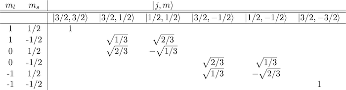
Now we return to 2p hydrogen with a small applied magnetic field: \hat{H}_B = \mu_B B (\hat{L}_z + 2 \hat{S}_z) Once again, I’ll invoke the result from perturbation theory that for sufficiently small B, we have for the energy shift E_{B,j,m} \approx \bra{j,m} \mu_B B (\hat{L}_z + 2 \hat{S}_z) \ket{j,m}. For the highest j=3/2 state, rewriting in the product basis is easy: E_{B,3/2,3/2} \approx \mu_B B \bra{1,1/2; 1,1/2} (\hat{L}_z + 2\hat{S}_z) \ket{1,1/2; 1,1/2} \\ = 2\hbar \mu_B B. The next lower state is harder, but not by much: E_{B,3/2,1/2} \approx \mu_B B \left( \frac{2}{3} \bra{1,1/2; 0,1/2} \hat{L}_z + 2\hat{S}_z \ket{1,1/2; 0,1/2} \right. \\ \left.+ \frac{1}{3} \bra{1,1/2;1,-1/2} \hat{L}_z + 2\hat{S}_z \ket{1,1/2; 1,-1/2} \right) \\ = \frac{2}{3} \hbar \mu_B B. We can keep going like this; I’ll let you work out the remaining energies yourself. The general result (for the 2p state only) turns out to be, compactly, E_{B,3/2,m} = \frac{4}{3} m \hbar \mu_B B, \\ E_{B,1/2,m} = \frac{2}{3} m \hbar \mu_B B. With the spin-orbit term, the spectral line associated with the 2p orbital of hydrogen splits according to j into two states; the addition of a small magnetic field breaks any remaining symmetry and splits all six states apart. And thanks to the formalism we’ve developed, we were able to easily calculate both terms, even though we had to work in two different bases to do so. Hopefully now you can appreciate the power of the Clebsch-Gordan coefficients!
We can sum up our result with the following sketch, assuming B is small enough that the magnetic splitting is smaller than the spin-orbit effect:
Here, you should complete Tutorial 6 on “Addition of spin-1/2 systems”. (Tutorials are not included with these lecture notes; if you’re in the class, you will find them on Canvas.)
14.5 Total angular momentum and reducible representations
When changing to the total angular momentum basis, our space has split into two separate spaces with total j=3/2 and j=1/2. The raising and lowering operators \hat{J}_{\pm} do not connect these two spaces together; we can think of now having two complete Hilbert spaces in terms of \hat{\vec{J}} that don’t overlap. This is in contrast to the original product basis, where we had to specify both m_l and m_s. In mathematical terms, our change of basis has decomposed a direct product (in which we require information from both the left and right spaces in order to describe a particular state) to a direct sum (in which the states can be in either the left or right space.)
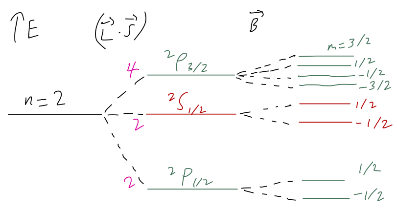
This can provide a drastic and useful simplification for many calculations involving angular momentum. For example, we know that the rotation matrix in the presence of both spin and angular momentum takes the form \hat{\mathcal{D}}(R) = \exp \left( \frac{-i (\hat{\vec{L}} \cdot \vec{n}) \phi}{\hbar} \right) \otimes \exp \left( \frac{-i (\hat{\vec{S}} \cdot \vec{n}) \phi}{\hbar} \right) = \exp \left( \frac{-i (\hat{\vec{J}} \cdot \vec{n}) \phi}{\hbar} \right). To really understand what we’re gaining in the total angular momentum basis, we have to think about what these actually look like as matrices if we write them out. In our original basis \ket{\ell s; m_\ell m_s}, if we try to rotate by some arbitrary angle, the matrix \bra{\ell s; m_\ell' m_s'} \hat{\mathcal{D}}(R) \ket{\ell s; m_\ell m_s} will be dense; all of the 36 entries will be non-zero. On the other hand, in the total angular momentum basis, we have the matrix \bra{j', m'} \exp \left( \frac{-i (\hat{\vec{J}} \cdot \vec{n}) \phi}{\hbar} \right) \ket{j, m}. Now imagine inserting the operator \hat{\vec{J}}^2 inside the matrix element; it will give \hbar^2 j(j+1) (...) acting to the right, and \hbar^2 j'(j'+1) (...) acting to the left. Since [\hat{\vec{J}}^2, \hat{\vec{J}}] = 0, these have to be equal, which means that either j=j', or the matrix element is zero! This means that rotations leave j unchanged, only mixing \hat{J}_z eigenstates together. In other words, the rotation matrix in total angular momentum basis becomes block diagonal:
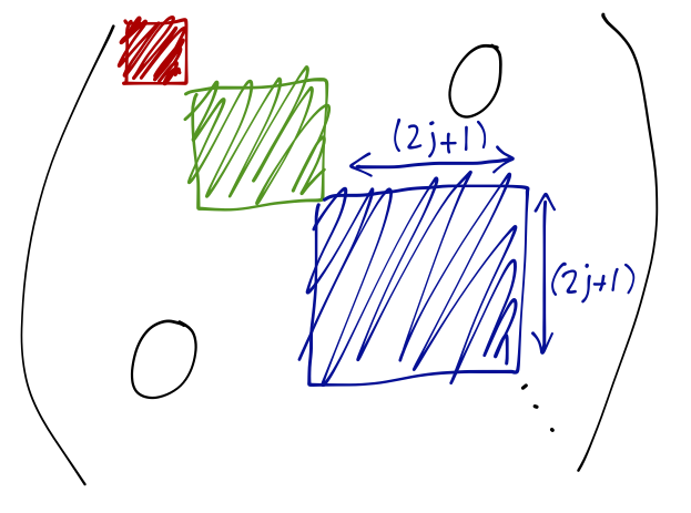
Each of the blocks rotates independently, as a single irreducible representation of the rotation group. The (2j+1) \times (2j+1) matrix that appears in each block is known as the Wigner D-matrix, {\mathcal{D}}_{m'm}^{(j)}(R) = \bra{j,m'} \exp \left( \frac{-i (\hat{\vec{J}} \cdot \vec{n}) \phi}{\hbar} \right) \ket{j,m} When we apply a rotation to our quantum system, the Wigner D-matrix tells us the amplitude for a rotated angular momentum eigenstate \ket{j,m} to be found in another angular momentum eigenstate \ket{j,m'}; by Born’s rule the probability of measuring \hat{J}_z' = m' after rotation is precisely |{\mathcal{D}}_{m'm}^{(j)}(R)|^2.
At this point, we can connect back to some math terminology, hopefully with a better intuition for what it means. The rotation matrix in the original product basis is generally dense (all entries are filled), but when we change to the total angular momentum basis, we find that it decomposes into a set of block-diagonal pieces that don’t transform into each other under rotation at all. The original matrix, which is a representation of the rotation group, is said to be reducible. The subsets of fixed j under the total angular momentum basis, on the other hand, are irreducible representations of rotation; they can’t be decomposed further. The problem of taking product representations and finding how they decompose into direct sums of irreducible representations is called tensor decomposition (or Clebsch-Gordan decomposition), and the good news for us is that the problem has been solved completely by mathematicians.
Let \mathbf{j} denote the representation of SO(3) (the rotation group) with angular momentum quantum number j and dimension d = 2j+1. The direct product of two such representations is decomposed as follows:
\mathbf{j_1} \otimes \mathbf{j_2} = \mathbf{|j_1 - j_2|} \oplus \mathbf{(|j_1 - j_2| + 1)} \oplus ... \oplus \mathbf{(j_1 + j_2)}.
This more sophisticated formula about representations gives us a quick and easy way to remember the selection rules for j when combining two angular momenta that we already found above; the results of our concrete Clebsch-Gordan solution also provide a more concrete way to reproduce this abstract formula.
Let’s apply this to our running example for 2p hydrogen to make sense of the notation. For that example we are combining orbital angular momentum with \ell = 1 and spin with s = 1/2; in the representation-theory notation, we have \mathbf{1} \otimes \mathbf{\tfrac{1}{2}} = \mathbf{\tfrac{3}{2}} \oplus \mathbf{\tfrac{1}{2}}. This matches the explicit change of basis we found above. Note also that we can check decompositions like this easily by using the dimensions. The dimension of a direct-product space is the product of the dimensions of the parts, so we get d = 3 \cdot 2 = 6 from the left-hand side above. On the right-hand side, we have a 4-dimensional representation and a 2-dimensional representation, giving us a total of 6 matching the left.
In this case, the results are pretty simple, but it can be more useful to do this quick cross-check once we get to higher spins. For example, using our tensor decomposition formula above we know that if we combine two spin-1 systems, the result is \mathbf{1} \otimes \mathbf{1} = \mathbf{2} \oplus \mathbf{1} \oplus \mathbf{0} or in terms of dimensions, 3 \times 3 = 5 + 3 + 1, which checks out.