21 Degenerate-state perturbation theory
Now that we’ve covered the basic formalism for time-independent perturbation theory, let’s tackle the problem of degeneracy. As we have seen, our formulas break down badly in the presence of degenerate unperturbed energy eigenstates. From the formalism we derived previously, we saw that our perturbation theory can be thought of as a series expansion in the ratio \frac{W_{nk}}{E_n^{(0)} - E_k^{(0)}}, where the labels n,k run over all distinct energy eigenstates and n \neq k. If we have an exact degeneracy, that is, if E_n^{(0)} = E_k^{(0)}, then this is obviously just nonsense. But even without an exact degeneracy, even just in the limit where the energies of two states become close together, this is clearly no longer small enough to expand in regardless of the size of our perturbative small parameter \lambda. However, this formula also suggests an obvious solution; we distinguished clearly in our derivation between the diagonal and off-diagonal matrix elements of W. If we can diagonalize W over the space of (near-)degenerate kets, then we will be able to proceed with our perturbative expansion as normal for the rest.
21.1 Two-state example
Let’s get a better feeling for what is happening by considering a simple two-state example. Suppose we have only two unperturbed states \ket{i^{(0)}} and \ket{j^{(0)}} which are degenerate, both with energy E_0. In the space spanned by these two states, we can write the full Hamiltonian (for these two states) as \hat{H} = \left(\begin{array}{cc} E_0 + \lambda W_{ii} & \lambda W_{ij} \\ \lambda W_{ji} & E_0 + \lambda W_{jj} \end{array}\right) We know nothing about the specific form of the perturbation, in particular it may be the case that W_{ii} \neq W_{jj}; what matters is that the energy levels are degenerate with \lambda=0. Since this is just a two-state system, we know how to solve the full Hamiltonian: recalling our general solution from Section 4.3, the energy eigenvalues are E_{\pm} = E_0 + \frac{\lambda}{2} (W_{ii} + W_{jj}) \pm \lambda \sqrt{\left( \frac{W_{ii} - W_{jj}}{2}\right)^2 + |W_{ij}|^2}. No trouble here; the energies split apart smoothly as \lambda is turned on. However, the eigenstates are a different matter. For the lower energy eigenstate \ket{E_-}, the solution is (assuming W is purely real) \ket{E_-} = \left( \begin{array}{c} -\sin (\theta/2) \\ \cos (\theta/2) \end{array}\right), where the mixing angle is equal to \tan 2\theta = \frac{|W_{ij}|}{W_{ii} - W_{jj}}. The dependence on \lambda cancels out entirely! So for any \lambda > 0, we have a discontinuous jump from the unperturbed eigenstates to the perturbed ones; there’s no way to write the state with the perturbation switched on as an order \lambda correction to the original state.
Now we come to the point: this discontinuity is not physical in any way, and we can get rid of it if we’re careful! First, notice that with \lambda = 0, we can write the Hamiltonian of this two state system as just \hat{H}_0 = \left(\begin{array}{cc} E_0 & 0 \\ 0 & E_0 \end{array}\right) This matrix is proportional to the identity, due to the degeneracy of the states \ket{i^{(0)}} and \ket{j^{(0)}}. But this means that there is an ambiguity as to what we call the energy eigenstates; any linear combination a \ket{i^{(0)}} + b \ket{j^{(0)}} is also an eigenstate with energy E_0. The perturbation \hat{W} breaks the ambiguity, by selecting a particular direction in terms of the \lambda-independent mixing angle \theta above.
So, the fix here is straightforward: we apply the \lambda-independent (but W-dependent) rotation first, while \lambda is still zero; then nothing strange happens as the perturbation is turned on. In fact, applying this rotation is precisely just diagonalizing the perturbation matrix \hat{W}. In the rotated basis, we’re just left with \hat{H} = \left(\begin{array}{cc} E_0 + \lambda W'_{i'i'} & 0 \\ 0 & E_0 + \lambda W_{j'j'} \end{array}\right) and now we’re actually just done, since we have diagonalized the full \hat{H}, which means we know its eigenstates and eigenvalues. (Typically, this two-by-two space will be a small subspace of a bigger problem, and we still have to use perturbation theory for the rest of the Hamiltonian.)
21.1.1 General procedure for degenerate PT
Since this is a critically important idea, let’s repeat it in a slightly different way. One of the keys to applying time-independent perturbation theory is that the effect of the perturbation is small, which means that all of our energy eigenstates after perturbation are equal to the \hat{H}_0 eigenstates plus a small correction, \ket{n} = \ket{n^{(0)}} + \lambda \ket{\delta_n}. In the degenerate case, the choice of \ket{n^{(0)}} itself becomes ambiguous until we switch \lambda on. To do our calculation correctly, we thus have to work backwards: we need to find the unique directions in the degenerate subspace which our perturbation \hat{W} picks out as eigenstates, and then find the \lambda \rightarrow 0 limit of those to identify the “correct” choices of unperturbed energy eigenstates.
In general, these states will be part of a larger Hamiltonian: \left( \begin{array}{cccc} E_0^{(0)} + \lambda \hat{W}_{ii} & \lambda W_{ij} & \lambda W_{ik} & ... \\ \lambda W_{ji} & E_0^{(0)} + \lambda \hat{W}_{jj} & \lambda W_{jk} & ... \\ \lambda W_{ki} & \lambda W_{kj} & E_k^{(0)} + \lambda \hat{W}_{kk} & ... \\ ... & ... & ... & ... \end{array}\right) We can diagonalize by rotating \ket{i} and \ket{j} to \ket{i'} and \ket{j'}, which changes the matrix in the corresponding columns and rows: \left( \begin{array}{cccc} E_0^{(0)} + \lambda E_{i'}^{(1)} & 0 & \lambda W_{i'k} & ... \\ 0 & E_0^{(0)} + \lambda E_{i'}^{(1)} & \lambda W_{j'k} & ... \\ \lambda W_{ki'} & \lambda W_{kj'} & E_k + \lambda \hat{W}_{kk} & ... \\ ... & ... &... & ... \\ \end{array} \right) With this rotation, the degeneracy is removed; our perturbation-theory formulas will be valid. All we have to do is make sure we apply everything using the new, rotated basis.
I should comment that “degenerate state perturbation theory” is actually something of an oxymoron. There’s no deep new formalism we had to derive here; the point is quite simply that perturbation theory doesn’t work on degenerate states. Remember that what we’re trying to do is find approximate solutions for the eigenvectors and eigenvalues of the full Hamiltonian \hat{H} = \hat{H}_0 + \lambda \hat{W}. All we’ve done here is recognized that this won’t work on a degenerate subspace, done the complete diagonalization within that subspace, and then used perturbation theory to study what happens to the rest of the states.
In particular, if we had a Hamiltonian which was completely degenerate, then we could only solve the full diagonalization problem, and then there would be nothing left to treat perturbatively! (Of course, high degrees of degeneracy usually indicate that there is a lot of symmetry in our system, in which case we have many other tools we can use to solve.)
21.2 Tips, tricks, and pitfalls in degenerate-state perturbation theory
The basic idea here is quite simple, but the reason degenerate-state perturbation theory is a completely separate chapter in my notes is that there are some subtle problems that can show up in the context of degeneracy and perturbation theory if we’re not careful, and there are also some useful tricks and methods that go beyond the simple idea of “diagonalize away the degeneracy” which are worth getting into a little bit.
21.2.1 Reminders about eigenstate and energy corrections
When we carry out our diagonalization procedure, we’re partly solving the problem we started with, namely finding the eigenstates and eigenvalues of the full \hat{H} = \hat{H}_0 + \lambda \hat{W}. This just means we have to be extra careful about keeping track of how the corrections appear.
First, we should always keep in mind that usually, the “diagonalized” states are still corrected at first order in \lambda. Notice that in our matrix above, \ket{i'} and \ket{j'} are not eigenstates of the full Hamiltonian; although we’ve diagonalized \hat{H}_0 + \lambda \hat{W} in their subspace, they still overlap with other non-degenerate states. If we write out the equation for the corrected states at first order, we see for example \ket{i'^{(1)}} = \sum_{k \neq i'} \ket{k^{(0)}} \frac{W_{ki'}}{E_{i'}^{(0)} - E_k^{(0)}} Our diagonalization removes the pathological W_{ij} term from the sum, but everything else remains, so we do expect to find order-\lambda corrections in general.
Second, the “diagonalized” energies are still corrected at first order in \lambda. Let’s write out the formula for the perturbative energy to second order: E_{i'} = E_{0}^{(0)} + \lambda W_{i'i'} + \lambda^2 \sum_{k \neq i'} \frac{|W_{i'k}|^2}{E_{i'}^{(0)} - E_k^{(0)}} + ... It just so happens that the first-order correction \lambda W_{i'i'} is usually computed as a byproduct of the diagonalization of the subspace, as we saw in our explicit two-state example from before; this is because the first-order correction only depends on the diagonal element W_{i'i'}. However, at second order, corrections from coupling of the perturbation to states outside the degenerate subspace show up again.
There is one term in the perturbative expansion which will not obviously blow up in the presence of degeneracy, namely the first-order energy correction, proportional to W_{ii}. Make sure you’re not studying a system with degenerate states if you’re only calculating first-order energy corrections! If there is a degeneracy and you don’t deal with it, your calculation will give you a “first-order” result in an expansion which is infinity at the next order - not very useful!
In fact, we have an example already written out here: go back up to the two-state example and think about what blindly applying the first-order formula E_i^{(1)} = W_{ii} would give you, versus what the full solution gives you at order \lambda.
Here, you should complete Tutorial 10 on “Degenerate-state perturbation theory”. (Tutorials are not included with these lecture notes; if you’re in the class, you will find them on Canvas.)
21.2.2 Near-degenerate perturbation theory
The states don’t have to be exactly degenerate for us to apply this method; they also don’t have to be exactly degenerate to cause problems in perturbation theory, since as we previously observed, convergence of the perturbative expansion requires \frac{\lambda |W_{ij}|}{E_i^{(0)} - E_j^{(0)}} \ll 1. If any two energies are extremely close to one another, then even if \lambda and \hat{W} are small the expansion will be poor. The good news is that if we have a near-degeneracy, we can do an approximate diagonalization of the corresponding subspace to greatly improve our perturbative series.
Suppose that we have two states \ket{E_m^{(0)}} and \ket{E_n^{(0)}} whose corresponding energies are nearly degenerate. We can then write E_m^{(0)} = \bar{E} - \epsilon, \\ E_n^{(0)} = \bar{E} + \epsilon, defining the average energy \bar{E} and the (half) difference \epsilon between the two energy values. By assumption, if they are nearly degenerate then we have \epsilon \ll \bar{E}.
Now, if these two states were exactly degenerate, then the state \ket{\psi} = \cos \theta \ket{E_m^{(0)}} - \sin \theta \ket{E_n^{(0)}} would still be an eigenstate of \hat{H}_0 for any mixing angle \theta. This is not true in the present case, but since the levels are nearly degenerate, we can rewrite the above as \hat{H}_0 \ket{\psi} = \cos \theta E_m^{(0)} \ket{E_m^{(0)}} - \sin \theta E_n^{(0)} \ket{E_n^{(0)}} \\ = \bar{E} \left[ \cos \theta \ket{E_m^{(0)}} - \sin \theta \ket{E_n^{(0)}} \right] + \epsilon \left[ \cos \theta \ket{E_m^{(0)}} + \sin \theta \ket{E_n^{(0)}} \right] where I’ve taken \bar{E} to be the average of the two energy values, and \epsilon to be their difference. So the rotated state \ket{\psi} is almost an eigenstate of \hat{H_0}, up to a small correction proportional to \epsilon.
This suggests how to proceed: we rewrite our Hamiltonian as \hat{H} = \hat{H}_0 + \lambda \hat{W} = \hat{H}_0' + \lambda \hat{W}' where \hat{H}_0' = \hat{H}_0 + \sum_{k=i,j} (\bar{E} - E_k^{(0)}) \ket{E_k^{(0)}}\bra{E_k^{(0)}} \\ \lambda \hat{W}' = \lambda \hat{W} + \sum_{k=i,j} (E_k^{(0)} - \bar{E}) \ket{E_k^{(0)}}\bra{E_k^{(0)}}. We’re just adding and subtracting the same term, of course, so \hat{H} is unchanged. After redefinition, \hat{H}_0' contains exactly degenerate states with energy \bar{E}, and our perturbation has picked up two additional terms proportional to the small parameter \epsilon. From here, we can proceed with exactly-degenerate perturbation theory. (You might worry about altering \hat{H}_0, but since the form of our small correction is exactly diagonal in the \ket{E_k^{(0)}} basis, they are still eigenstate of \hat{H}_0' and we can rely on everything we know about solving the unperturbed system.)
21.2.3 Higher-order degeneracies
If the off-diagonal terms W_{ij} vanish in a degenerate subspace, then our diagonalization procedure itself becomes ambiguous, and we are back to the problem we started with that a discontinuity will appear between the perturbed and unperturbed states. In this situation, the higher-order terms in \lambda arising from interaction with the other states have to break the degeneracy.
Dealing with higher-order degeneracy can get very confusing in practice, since the details are subtle (in Sakurai, the discussion is given in the form of a homework problem “for the experts”.) I won’t go through all of the details here, but to at least understand what the procedure is for dealing with such a case, it’s simplest to revisit the formal solution and see how it needs to be repaired for the case of degeneracy. Our starting point is the rearranged equation (E_n^{(0)} - \hat{H}_0) \ket{n} = (\lambda \hat{W} - \Delta_n) \ket{n}. To formally solve for \ket{n} before, we encountered the inverse operator (E_n^{(0)} - \hat{H}_0)^{-1}, and to make sure that it existed we defined the projection operator \hat{\phi}_n to select out the eigenstate \ket{n^{(0)}} which makes the inverse blow up. Now that we have a degeneracy, we can approach the solution in the same way, but we have to write a bigger projector operator.
Suppose that we have a set of generate states \ket{n_i^{(0)}}, with i = 1, ..., d, all with the same energy E_D^{(0)}. These states span a degenerate subspace of our Hilbert space \mathcal{D} \subset \mathcal{H}. Let’s define a projector \hat{\mathcal{P}} \equiv \sum_{j \in \mathcal{D}} \ket{n_j^{(0)}} \bra{n_j^{(0)}} and then the complementary projector is \hat{Q} \equiv 1 - \hat{\mathcal{P}} = \sum_{k \notin \mathcal{D}} \ket{k^{(0)}} \bra{k^{(0)}}.
Now, what we want to do is isolate the degenerate subspace part of \ket{n} from the rest of it. We can always divide up as follows: \ket{n} = \hat{P} \ket{n} + (1-\hat{P}) \ket{n} \equiv \ket{n_P} + \ket{n_Q}. Now we go back to the starting equation and start applying projectors. First, we have \hat{P} (E_n^{(0)} - \hat{H}_0) \ket{n} = \hat{P} (\lambda \hat{W} - \Delta_n) \ket{n} The left-hand side is exactly zero, acting to the left with \hat{H}_0 on the projector, so this becomes 0 = \hat{P} (\lambda \hat{W} - \Delta_n) (\ket{n_P} + \ket{n_Q}) \\ \Delta_n \ket{n_P} = \lambda \hat{P} \hat{W} \ket{n_P} + \lambda \hat{P} \hat{W} \ket{n_Q}. Now let’s look at the other projection: \hat{Q} (E_n^{(0)} - \hat{H}_0) \ket{n} = \hat{Q} (\lambda \hat{W} - \Delta_n) \ket{n} \\ (E_n^{(0)} - \hat{H}_0) \ket{n_Q} = \hat{Q} (\lambda \hat{W} - \Delta_n) (\ket{n_P} + \ket{n_Q}) \\ \Rightarrow \ket{n_Q} = \frac{\hat{Q}}{E_n^{(0)} - \hat{H}_0} (\lambda \hat{W} - \Delta_n) (\ket{n_P} + \ket{n_Q}). This equation, combined with the one above for \ket{n_P}, gives us a linear system of equations for the components \ket{n_P} and \ket{n_Q}. Although I won’t try to do it formally, it should be clear that we can always plug this equation into the last one and eliminate \ket{n_Q} to rewrite the equation for \ket{n_P} in the form \hat{\Delta}_n \ket{n_P} = \hat{H}_{\rm eff} \ket{n_P}. In other words, the components of \ket{n} within the degenerate subspace satisfy an eigenvalue equation for an operator known as the effective Hamiltonian, \hat{H}_{\rm eff}. The effective Hamiltonian gets more and more complicated as we go to higher orders, but if we work order by order in \lambda it’s straightforward to work out. As a first test, let’s start at lowest order. Since \ket{n_Q} itself is of order \lambda while \ket{n_P} is \mathcal{O}(1), to lowest order we just have \lambda E_n^{(1)} \ket{n_P} = \lambda \hat{P} \hat{W} \ket{n_P} + \mathcal{O}(\lambda^2) from which we read off that \hat{H}_{\rm eff}^{(1)} = \lambda \hat{P} \hat{W} \hat{P} (where it is typically written using projectors on both sides to emphasize that we’re solving only in the degenerate subspace.) This also tells us what we found above more directly, which is that the eigenvalues resulting from diagonalizing \hat{W} in the degenerate subspace are exactly the first-order energy corrections.
Since we’re set up the formalism clearly, it’s very easy now to see what happens at higher order. If we continue to order \lambda^2, then we have to keep the first term in the \ket{n_Q} equation we found, which leads to \lambda^2 E_n^{(2)} \ket{n_P} = \lambda^2 \hat{P} \hat{W} \frac{\hat{Q}}{E_n^{(0)} - \hat{H}_0} \hat{W} \ket{n_P} or \hat{H}_{\rm eff}^{(2)} = \lambda^2 \hat{P} \hat{W} \frac{\hat{Q}}{E_n^{(0)} - \hat{H}_0} \hat{W} \hat{P}. This expression matches the result given in Gottfried and Yan’s textbook (equation 274), where you can find further discussion.
In general, the punchline of this whole discussion is that to avoid anything discontinuous happening as \lambda \rightarrow 0, the degenerate states \ket{n_P^{(0)}} have to be rotated so that they are eigenvectors of whatever the lowest-order nonzero piece of \hat{H}_{\rm eff} is. Under normal circumstances, this is \hat{P} \hat{W} \hat{P}, the part of \hat{W} itself that is in our degenerate subspace. But if that is zero, we compute the second-order effective Hamiltonian and diagonalize that instead to find the correct rotation.
Consider the following Hamiltonian, a variation on the one we studied on the tutorial above: \hat{H} = \left( \begin{array}{ccc} E_0 & 0 & \lambda a \\ 0 & E_0 & \lambda a \\ \lambda a^\star & \lambda a^\star & E_1 \end{array}\right) with basis states \{\ket{i}, \ket{j}, \ket{k}\} in order. Calculate the first-order corrected eigenstates, and compare to the results of exactly diagonalizing the matrix.
Answer:
Answer to be filled in, but essentially the same system is studied in Gottfried and Yan so you can find the answer there in the meantime.21.2.4 Symmetries and degeneracy
Sometimes, even going to second order in perturbation theory isn’t good enough, or third order; it is in fact possible for the perturbation to fail to lift the degeneracy between energy eigenstates to all orders in perturbation theory. This is actually good news and not bad; the vanishing of perturbative corrections to all orders typically signals the presence of an underlying symmetry.
Remember that our basic problem with degenerate states was that a discontinuous jump could appear when we switch on \lambda, since there are many ways to write our unpertubed basis in the degenerate subspace. But if there is another operator \hat{A} so that [\hat{A}, \hat{H}] = 0, then there is no ambiguity between perturbed and unperturbed states; we can label the perturbed energy eigenstates with the eigenvalues of \hat{A}.
This will save us a lot of trouble in the hydrogen atom; for example, if we consider any perturbation which commutes with \hat{L}_z of the electron, then we can use m_l to label the perturbed eigenstates, and the perturbation will already be diagonal and unambiguous.
Another way to state what is happening here is: in cases where all off-diagonal matrix-elements vanish due to a symmetry, we are protected from any perturbative corrections appearing, and simple diagonalization in our degenerate subspace ends up becoming an exact solution of that part of the system.
Now that we’re fully equipped to handle problems with degeneracy, we’re ready to tackle some examples. A particularly interesting physical system with degeneracies is the hydrogen atom. Before we get into the perturbation theory, let’s do a quick review of the basic hydrogen solutions.
21.3 Review of the hydrogen atom solution
As discussed previously, I don’t include a solution of the hydrogen atom in these notes; it’s a common enough textbook example, as well as a very special case. If you really want to see the details of the solution, I recommend chapter 13 of Shankar. I will be drawing on a lot of notation and results from back in Chapter 12 below, so if you don’t recognize something go back and look at those materials again.
Since hydrogen is one of the few cases where we can find an analytic solution in quantum mechanics, there is a lot of interesting physics that relies on using the hydrogen atom as \hat{H}_0, so let’s review the key results. It’s useful to slightly generalize and consider the solution for a “hydrogenic” atom, i.e. a bound state of a single electron (charge -e) with a nucleus of total charge +Ze. The corresponding Coulomb potential is V(r) = -\frac{Ze^2}{r}. This is a central and spherically symmetric potential, which we solve in three dimensions. Following the formalism we developed previously for such systems, we know that energy eigenfunctions (solutions to the time-independent Schrödinger equation) will decompose into radial and angular components, \psi_{nlm}(r, \theta, \phi) = R_{nl}(r) Y_l^m(\theta, \phi). We see that the energy eigenstates can be written as \ket{nlm}, where l and m are the quantum numbers associated with angular momentum operators \hat{L}^2 and \hat{L}_z respectively. The other quantum number n is known as the principal quantum number, and it is what determines the energy eigenvalues, E_n = -\frac{1}{2} mc^2 \frac{Z^2 \alpha^2}{n^2}, where we have defined the fine-structure constant \alpha \equiv \frac{e^2}{\hbar c}. These are all negative, as you would expect for an electron in a bound state under the Coulomb potential (which is also strictly negative for all r.) For hydrogen’s ground state with Z=n=1, the resulting energy is -13.6 eV.
Aside from the usual restrictions l \geq 0 and |m| \leq l which are generic for angular momentum operators, the hydrogen solutions also satisfy the conditions n \geq 1;\ \ \ l < n. This means that the ground state n=1 is unique with l=0 (in spectroscopic notation, the 1s state.) For n=2, we have both l=0 (2s) and l=1 (2p) states, four distinct \ket{2lm} states in total, leaving us with a four-fold degeneracy.
The radial solutions can be written in terms of confluent hypergeometric functions F(a;c;\rho), which reduce in certain cases to the associated Laguerre polynomials L_p^q(\rho). The fully general formula, following Sakurai’s notation, is R_{nl}(r) = \frac{1}{(2l+1)!} \left( \frac{2Zr}{na_0}\right)^l e^{-Zr / (na_0)} \\ \times \sqrt{ \left( \frac{2Z}{na_0} \right)^3 \frac{(n+l)!}{2n(n-l-1)!} } F\left(-n+l+1; 2l+2; \frac{2Zr}{na_0} \right) and here it is again conveniently in Mathematica code:
R[n_, l_] := 1/(2*l + 1)!*((2*Z*r)/(n*a0))^l*Exp[(-Z*r)/(n*a0)]*
Sqrt[((2*Z)/(n*a0))^3*(n + l)!/(2 n*(n - l - 1)!)]*
Hypergeometric1F1[-n + l + 1, 2 l + 2, (2*Z*r)/(n*a0)];
The ground-state solution n=1, l=0 is simple enough to write in terms of elementary functions, and is worth having available: R_{10}(r) = 2 \sqrt{\frac{Z^3}{a_0^3}} e^{-Zr/a_0}. Don’t forget that this is only the radial part of the wavefunction: if we want to write the total wavefunction \psi_{100}(r,\theta, \phi), we multiply by the spherical harmonic Y_0^0 = 1/\sqrt{4\pi}. A unique feature of the ground-state wavefunction, as well as all higher l=0 wavefunctions, is that they don’t vanish at the origin, R_{n0}(0) \neq 0. Higher-l wavefunctions all vanish at the origin, with the electron being “pushed away” by the centrifugal barrier as we saw in general before.
In addition to Z and quantum numbers, these solutions depend on the quantity a_0, which is known as the Bohr radius. In terms of more fundamental quantities, the Bohr radius is given by a_0 = \frac{\hbar^2}{m_e e^2}. The value of the ground-state n=1 energy, given as 13.6 eV above, is sometimes used as a unit of energy known as the Rydberg, with symbol “Ry”: in terms of other quantities defined so far, 1\ {\rm Ry} = 13.6\ {\rm eV} = \frac{m_e e^4}{2\hbar^2} = \frac{e^2}{2a_0}.
21.3.1 Example: nucleus finite-size correction
Let’s warm up with a simple non-degenerate perturbation theory example by considering the correction to the ground state energy coming from the finite size of the nucleus. The Coulomb potential we wrote above assumes the nucleus is a point charge, but of course if we look closely enough, we will find that it has some non-zero extent. Treating the nucleus as a uniform ball of charge with finite radius r_0, then the potential is corrected to V(r) = \begin{cases} -\frac{Ze^2}{r}, & r \geq r_0; \\ \frac{Ze^2}{2r_0} \left[ \left( \frac{r}{r_0}\right)^2 - 3 \right], & r \leq r_0. \end{cases} We can thus rewrite our Hamiltonian as \hat{H} = \hat{H}_0 + \lambda \hat{W}, where \hat{W} = \begin{cases} 0, & r \geq r_0; \\ \frac{Ze^2}{2r_0} \left[ \left( \frac{r}{r_0}\right)^2 - 3 + \frac{2r_0}{r} \right], & r \leq r_0. \end{cases} where this time I am using \lambda=1 purely as an auxiliary constant and just ignoring it. Why is it valid to treat this correction perturbatively if \lambda = 1? We know that the nucleus is very small, and so we expect that the overlap of the electron wavefunction with the region we’re changing the potential in is quite small. We will find that the matrix elements of \hat{W} depend on the ratio r_0 / a_0. The small size of this ratio validates our perturbative expansion; for hydrogen, a_0 \sim 10^{-10} m, while the charge radius of the proton is closer to 10^{-15} m.
(If you aren’t happy with playing fast and loose with the perturbative expansion like this, then you can define \lambda \equiv r_0 / a_0 and factor it out of the perturbation to make it more explicit. The final results will be the same.)
To compute the energy shift due to this finite-size effect, we have to integrate using hydrogenic wavefunctions. Looking at the ground state \ket{nlm} = \ket{100}, we have for the first-order energy correction E_{100}^{(1)} = \bra{100} \hat{W} \ket{100} \\ = \int_0^{r_0} dr\ r^2 |R_{10}(r)|^2 \frac{Ze^2}{2r_0} \left[ \left( \frac{r}{r_0} \right)^2 - 3 + \frac{2r_0}{r} \right] \\ = \frac{2Z^4e^2}{r_0 a_0^3} \int_0^{r_0} dr\ r^2 \left[ \left( \frac{r}{r_0} \right)^2 - 3 + \frac{2r_0}{r} \right] e^{-2r/a_0} (ignoring the angular integration which is handled by the normalization of the spherical harmonics.) This is a straightforward integral, which you can do in Mathematica or with integral tables. The result, as promised, depends on the small ratio r_0 / a_0. Although taken at face value, the energy shift will contain higher powers of r_0 / a_0, we know that we’re only working at first order here we should really only keep the first term in a series expansion; doing so gives the result E_{100}^{(1)} = \frac{2Z^4 e^2 r_0^2}{5 a_0^3} = \frac{4}{5} Z^4 \left( \frac{r_0}{a_0}\right)^2\ {\rm Ry}. The correction is therefore of order (r_0 / a_0)^2, i.e. a 10^{-10} effect for the hydrogen atom; very small indeed!
This is, in fact, the largest correction factor out of all of the states of hydrogen; we know that for higher n or higher l, the wavefunction of the electron will be localized further away from the origin, and they will turn out to be suppressed by further powers of (r_0 / a_0). On the other hand, the correction grows rapidly as the charge of the nucleus increases, and this isn’t even including the fact that the nuclear radius r_0 also increases for higher-Z atoms as the nucleus contains more and more protons. So in sufficiently precise atomic physics experiments with larger nuclei, this is not always negligible.
Replacing the electron with a muon, the electron’s heavier cousin, can also lead to appreciable effects by greatly reducing the orbital radius; in fact, looking for the small finite-size correction to the energy spectrum of muonic hydrogen is one approach to measuring the radius of the proton experimentally.
21.4 Hydrogen in electromagnetic fields
We now have the tools necessary to study the response of a hydrogenic atom to being placed into a background electric or magnetic field. Electric fields are somewhat more straightforward; they will add a linear perturbation to the electron’s potential, breaking the rotational invariance and causing the degenerate \ket{lm} energy levels to split apart. Magnetic fields also cause energy levels to split apart, but they couple to both the orbital motion and to the spin of the electron, so the way that the energy splittings appear is a bit more complicated.
With both an applied electric and magnetic field, taken to be weak and uniform background fields, the hydrogenic Hamiltonian is modified to: \hat{H} = -\frac{Ze^2}{r} + e \vec{E} \cdot \hat{\vec{r}} + \frac{e}{2m} \vec{B} \cdot (\hat{\vec{L}} + 2\hat{\vec{S}}).
The words “weak and uniform” are very important in the above Hamiltonian. First of all, even in constant background fields there is a quadratic term proportional to |B|^2; we ignore that simply because we assume that doing perturbation theory, the B-field is weak enough that it will be negligible. We also assume that the electromagnetic fields are constant in space, meaning their gradients are negligible over the scale of an atom - this is often a reasonable assumption, but there can be situations where the field gradient terms matter. Finally, we also assume the fields are uniform in time (i.e. constant). The case of time-dependent electromagnetic fields is very important to study (the main application being to a light wave impinging on an atom), but we aren’t prepared to look at it yet.
Further details (including dealing with time-dependent electromagnetic fields) can be found in David Tong’s notes on atoms in electromagnetic fields.
It’s easy to get badly confused about minus signs running around in these sorts of calculations, since we have plugged in the electron charge q=-e, which is negative. For the electric field, a good way to check the sign is to let \vec{E} = |\mathbf{E}| \hat{z}, so that the potential is tilted upwards for positive z and down for negative z; this tends to accelerate the electron in the direction of negative z, opposite the field direction. This is the correct direction of motion, since the force \vec{F} = q\vec{E} points opposite the electric field for a negative charge. (This does not match the copy of Sakurai on my desk, equation (5.2.17); I suspect there is a mistake, although the physics we’re about to study doesn’t really change significantly, just the identification of which states pick up positive or negative corrections in some cases.)
21.4.1 Applied electric fields (ground state)
Let’s begin with the case where there is just a uniform background electric field oriented in the z direction, \vec{E} = |\textbf{E}| \hat{z}. The corresponding perturbation to the Hamiltonian is then, from above, \hat{W} = e|\textbf{E}| \hat{z}. Here the perturbation is \vec{E} itself, which we assume that we’re controlling with a dial in our laboratory so that it remains “small”, in the sense that matrix elements involving \vec{E} will give small energy corrections relative to the existing energy splittings of our atom. (This means we don’t have to bother with a dimensionless \lambda at all, although if you want to be more neat about units, you could introduce it and write something like |\textbf{E}| = \lambda |\textbf{E}_0|, where maybe |\textbf{E}_0| is the full-strength magnetic field in your lab for example.)
There is a subtlety to this particular perturbation; because it is linear in z, we find \hat{W} \rightarrow -\infty as z \rightarrow -\infty. This means that technically, it’s possible for our formerly bound electron to escape the hydrogen atom completely due to the applied field. We can ignore this complication, partly because in reality the electric field doesn’t actually have infinite extent and in the region where it is present, it won’t be strong enough for appreciable tunnelling to happen if |\mathbf{E}| is small enough.
We don’t have to ignore this effect either - another application of perturbation theory here that could be interesting is calculating the lifetime of the electron states with non-zero |\mathbf{E}|. But the effect is only really significant for highly excited electronic orbitals, anyway.
In general, the treatment of an electric-field perturbation on the hydrogen atom requires degenerate-state perturbation theory, since all of the hydrogen energy levels are n^2-fold degenerate. But the 1s ground state is the sole exception, since it is non-degenerate (ignoring the electron spin), which means we can treat the ground-state correction as a non-degenerate problem.
To write this without the notation becoming too cumbersome, let’s label all of the unperturbed hydrogen energy levels with a single integer label \ket{k^(0)}, with \ket{1^{(0)}} \equiv \ket{100} denoting the ground state. To second order, the correction to the ground-state energy is given by \Delta E = +e |\mathbf{E}| z_{11} + e^2 |\mathbf{E}|^2 \sum_{k \neq 1} \frac{|z_{1k}|^2}{E_1^{(0)} - E_k^{(0)}}.
The first term above, z_{11} = \bra{100} \hat{z} \ket{100}, is easily seen to vanish identically; although the electric field breaks parity, the original Hamiltonian is parity invariant, and so the ground state \ket{1^{(0)}} is a parity eigenstate. Since the operator \hat{z} is itself odd, it’s easy to see that \left\langle \hat{z} \right\rangle = 0. Physically, this corresponds to the fact that the spherically-symmetric hydrogen atom does not have an electric dipole moment, as we argued before.
However, as we mentioned the electric field itself breaks parity, causing polarization of the charge distribution. This effect results in an energy shift which depends quadratically on the electric field, since the induced dipole moment is itself proportional to |\mathbf{E}|: \Delta E = -\frac{1}{2} \alpha_E |\mathbf{E}|^2. The coefficient \alpha_E is the electric polarizability, which we’ve encountered before briefly in the ammonia maser example. We can read the polarizability of the atomic ground state off from the expansion above: \alpha_E = -2e^2 \sum_{k>1} \frac{ |\bra{k^{(0)}} \hat{z} \ket{1^{(0)}}|^2 }{E_1^{(0)} - E_k^{(0)}}. (Incidentally, the set of higher states \ket{k^{(0)}} includes all of the unbound states of the electron as well. If we really wanted to treat things rigorously here, we would have to write this as a sum plus an integral.)
Instead of trying to evaluate this precisely, let’s resort to some tricks to get a reasonable estimate. Since we’re considering the ground state, notice that we have an upper bound on the sum, \sum_{k>1} \frac{ |\bra{k^{(0)}} \hat{z} \ket{1^{(0)}}|^2 }{E_1^{(0)} - E_k^{(0)}} < \frac{1}{E_1^{(0)} - E_2^{(0)}} \sum_{k>1} |\bra{k^{(0)}} \hat{z} \ket{1^{(0)}}|^2 since all of the other energy differences are larger than the one we’ve factored out. But notice that this second sum is much easier to evaluate: we can write \sum_{k>1} |\bra{k^{(0)}} \hat{z} \ket{1^{(0)}}|^2 = \sum_{\textrm{all}\ k} |\bra{k^{(0)}} \hat{z} \ket{1^{(0)}}|^2 \\ = \left\langle \hat{z}^2 \right\rangle where we’ve just used completeness in the last step. Now we invoke rotational invariance: for the ground state, we must have \left\langle \hat{z}^2 \right\rangle = \left\langle \hat{x}^2 \right\rangle = \left\langle \hat{y}^2 \right\rangle = \frac{1}{3} \left\langle \hat{r}^2 \right\rangle. This last expectation value we can evaluate directly from the wavefunction: \left\langle \hat{r}^2 \right\rangle = \int_0^{\infty} dr\ r^2 |R_{10}(r)|^2 r^2 \\ = \int_0^{\infty} dr\ \frac{4r^4}{a_0^3} e^{-2r/a_0} \\ = \frac{a_0^2}{8} \int_0^{\infty} d\rho\ \rho^4 e^{-\rho}. We can evaluate this integral by integrating by parts repeatedly, taking derivatives of the polynomial term; the boundary terms at 0 and \infty always vanish, until we end up with \left\langle \hat{r}^2 \right\rangle = \frac{a_0^2}{8} \int_0^{\infty} d\rho\ (24 e^{-\rho}) = 3a_0^2, and so \left\langle \hat{z}^2 \right\rangle = a_0^2. (Note: the corresponding formula in Sakurai has a typo.) Writing E_1^{(0)} - E_2^{(0)} = -\frac{3}{4}\ {\rm Ry} = -\frac{3e^2}{8a_0}, we can combine our results to find \alpha_E < \frac{16a_0}{3} (a_0^2) \approx 5.3 a_0^3. We can also find a lower bound on \alpha_E just by evaluating the first term in the sum, since all of the terms are positive-definite. This is readily done by computing the overlap \bra{210} \hat{z} \ket{100} (the other three n=2 states all give zero); you should find, putting in the constants, the bound \alpha_E \gtrsim 3.0 a_0^3.
Although these bounds are relatively simple to find, it is in fact possible to carry out the complete sum/integral; this is far too elaborate to go through here, but the exact result for hydrogen turns out to be \alpha_E = 4.5 a_0^3, which agrees well with experimental determinations. (This is far larger than the polarizability of a uniform classically charged sphere, which would be just a_0^3.)
Our Hamiltonian here describes just the orbital electron in isolation, subject to the electric field of the proton at the center of the atom. However, it’s useful to remember that we’re describing a hydrogen atom, which is a neutral object; with zero charge, the hydrogen atom doesn’t couple directly to the electric field applied to it. But despite having no net charge, the hydrogen atom isn’t just a neutral sphere; in general, since its components are charged, it will have an electric dipole moment \vec{d}, which in a background electric field gives an energy contribution of \Delta E = -\vec{d} \cdot \vec{E}. For excited electron orbitals, the electron’s orbit is not perfectly spherical, and there will generally be a non-zero dipole moment, giving a linear contributon in |\vec{E}| to its energy. But in the ground state (and in all s-wave states), the orbital is perfectly spherical, so rotational symmetry forbids the presence of a non-zero dipole moment.
However, the hydrogen atom doesn’t consist of fixed components; in the presence of an electric field, the proton will feel a force along the direction of \vec{E}, while the electron will be pulled in the opposite direction. This induces a dipole moment, by deforming the charge distribution along the direction of the electric field, and the resulting dipole moment then couples to the electric field. This gives rise to a quadratic correction in |\vec{E}|, as we found above.
I’ll note in passing that historically, this energy splitting is known as the “quadratic Stark effect”, while the “linear Stark effect” is a linear response to an applied background electric field that we’re about to study.
21.4.2 Applied electric fields (excited states)
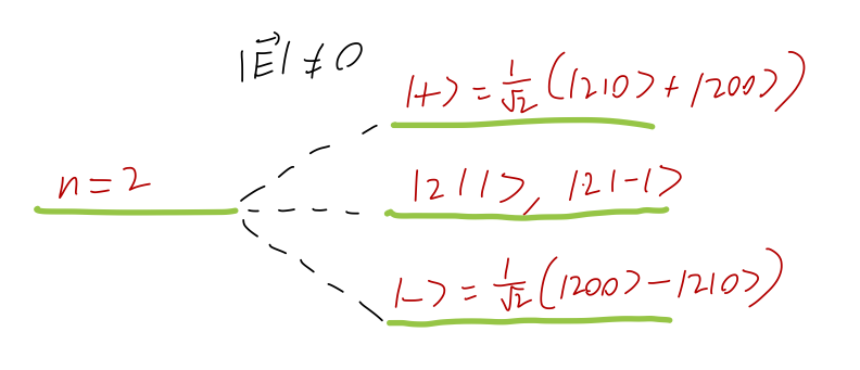
Let’s continue with the same perturbation \hat{W} = e |\mathbf{E}| \hat{z}. and move on to see what happens to the n=2 states. Here we find four states that are degenerate: the l=1 triplet (aka 2p) and the l=0 singlet (2s). Once again, parity simplifies the discussion: since \bra{nl'm'} \hat{z} \ket{nlm} \rightarrow -(-1)^{l'-l} \bra{nl'm'} \hat{z} \ket{nlm} under a parity transformation, the perturbation will only have non-vanishing matrix elements between l=0 and l=1 states. We also recognize \hat{z} as the q=0 component of the spherical position tensor \hat{r}_q^{(1)}, which means that we must also have m=m'. Based on these two selection rules, for the n=2 energy level there is only one non-vanishing matrix element: \hat{W} = \left( \begin{array}{cccc} 0 & \bra{200} \hat{W} \ket{210} & 0 & 0 \\ \bra{210} \hat{W} \ket{200} & 0 & 0 & 0 \\ 0 & 0 & 0 & 0 \\ 0 & 0 & 0 & 0 \end{array} \right) with the column vectors taken to be \ket{200}, \ket{210}, \ket{21(-1)}, \ket{211} in order. This is a degenerate-state perturbation theory problem - all four states have unperturbed energy E_2 - so we have to diagonalize in the m=0 states. Since the matrix is so simple, we see immediately that the correct eigenkets are \ket{\pm} = \frac{1}{\sqrt{2}} (\ket{200} \pm \ket{210}), and the first-order energy corrections are given by the resulting diagonal entries \Delta_{\pm}^{(1)} = \pm \bra{200} \hat{W} \ket{210} = \pm e |\mathbf{E}| \bra{200} \hat{z} \ket{210}. As we saw before, there’s no easy way to evaluate general matrix elements of \hat{z} between hydrogen levels; we’ll use the explicit formulas here. We can rewrite z = r \cos \theta, and as always the integral splits into an angular part and a radial part. For the angular integral, we have \int d\Omega (Y_1^0)^\star(\theta, \phi) \cos \theta Y_0^0(\theta, \phi). Inspecting the definitions of the harmonics, we see that Y_1^0 is proportional to \cos \theta; in fact, Y_1^0(\theta, \phi) = \sqrt{3} \cos \theta Y_0^0(\theta, \phi), which allows us to use the orthogonality of the spherical harmonics to evaluate the integral: \int (...) = \frac{1}{\sqrt{3}}. For the radial integral, you’ll have to go back and look up the form of the wavefunctions; I’ll just tell you that the result is -3 \sqrt{3} a_0. Combining, we have that \Delta_{\pm}^{(1)} = \mp 3 e a_0 |\mathbf{E}| . A diagram showing the splitting of the n=2 energy level due to the electric field is applied is shown below.
By the way, this was really a problem in nearly degenerate perturbation theory; the \ket{200} and \ket{210} states don’t have the same energy in reality, due to other effects we’ve ignored. In fact, they’re not even energy eigenstates; we know that the spin-orbit coupling splits \ket{210} into two energy levels, {}^2P_{1/2} and {}^2P_{3/2}. Our calculation is only valid in the limit that |\mathbf{E}| is large compared to these effects (but still small enough compared to the orbital energy differences in hydrogen that we can use perturbation theory.)
21.4.3 Applied magnetic fields
Now let’s turn to the effects of an applied magnetic field on hydrogen. The perturbing Hamiltonian is now \hat{W}_B = \frac{eB}{2m_e c} (\hat{L}_z + 2 \hat{S}_z) This time, we obviously need to include the spin of the electron as well, so we label our eigenstates by \ket{n,l,m,m_s}. If this perturbation was the only interaction, then we would be able to stay in this basis and calculate; the perturbation above is already diagonal in the given basis. However, we know that the spin-orbit coupling \hat{\vec{S}} \cdot \hat{\vec{L}} splits the energy levels of hydrogen based on their total angular momentum \hat{\vec{J}} = \hat{\vec{L}} + \hat{\vec{S}} eigenvalues (as we discussed for 2p hydrogen back in Section 14.3, and will discuss in general shortly.) Assuming that our magnetic field is truly small, even compared to the spin-orbit energy corrections, we must change basis: \ket{nlm_l m_s} \rightarrow \ket{nljm} Studying this case in general requires some more machinery related to rotational symmetry (namely, the Wigner-Eckart theorem), so we’ll defer studying the very weak-field case. Instead, we’ll assume that B is large enough that the spin-orbit coupling is negligible, but not so large that perturbation theory is unreliable. In this limit, the resulting energy splittings are known as the Paschen-Back effect.
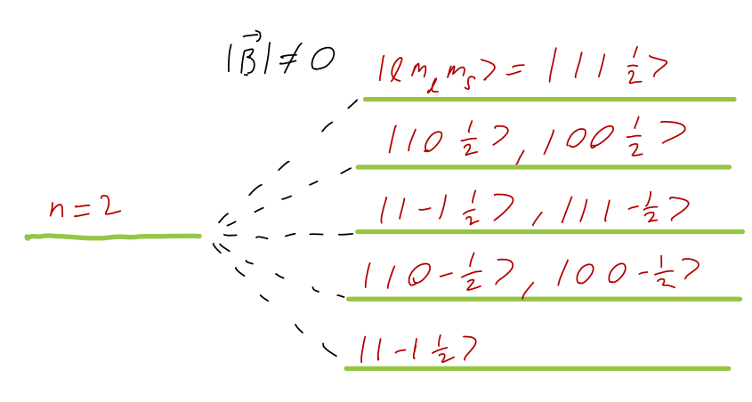
With the spin-orbit term neglected, we’re free to work in the \ket{n l m_l m_s} basis. This is great news since our perturbation is already diagonal for these states: we find immediately that \Delta E = \bra{nlm_l m_s} \hat{W}_B \ket{nlm_l m_s} = \frac{eB\hbar}{2m_e c} (m_l + 2m_s).
If we go back to think about the n=2 energy level, then m_l = \{-1, 0, 1\} and m_s = \pm \tfrac{1}{2} splits the overall state into five different levels: