2 Hilbert spaces and postulates of QM
Now that we’ve established what features are needed in quantum mechanics - namely, interference effects and complex-valued physical quantities - we’ll learn a bit about the mathematics of Hilbert spaces, which will give us the language we need to understand these effects. Once we have this, we can write down a set of foundational postulates for quantum mechanics.
My presentation of Hilbert spaces will be fairly practical and physics-oriented. If you have a strong math background and are interested in a more rigorous treatment, I direct you to this nice set of lecture notes from N.P. Landsman. The textbook “Analysis” by Elliott Lieb and Michael Loss was also recommended to me by a previous student.
2.1 Hilbert spaces
Let’s start with a definition:
A Hilbert space \mathcal{H} is a vector space which has two additional properties:
- It has an inner product, which is a map that takes two vectors and gives us a scalar (a real or complex number.)
- All Cauchy sequences are convergent. (This isn’t a math class, so we won’t dwell on this property, but roughly, it guarantees that there are no “gaps” in our space.)
Regular and familiar vector spaces, like \mathbb{R}^3 (the space of coordinate vectors), are also Hilbert spaces. The extra formalism sitting underneath Hilbert space lets us comfortably deal with spaces with any number of dimensions, including infinite dimensions, which we will need when we talk about continuous variables like position and momentum.
Let’s define our notation. We will use the “bra-ket” notation introduced by Paul Dirac. Vectors in the Hilbert space \mathcal{H} will be written as kets, \ket{\alpha} \in \mathcal{H}. I may use the words “vector” and “ket” interchangeably, but I’ll try to stick to “ket”. Adding two kets gives another ket and works normally (if you’re more mathematically inclined, it is commutative and associative.) Like any other vector space, Hilbert space also includes the product of a number c (also known as a scalar) with a ket, which gives another ket satisfying the following rules: (c_1 + c_2) \ket{\alpha} = c_1 \ket{\alpha} + c_2 \ket{\alpha} \\ c_1 (c_2 \ket{\alpha}) = (c_1 c_2) \ket{\alpha} \\ c (\ket{\alpha} + \ket{\beta}) = c \ket{\alpha} + c \ket{\beta} \\ 1 \ket{\alpha} = \ket{\alpha} For quantum mechanics, we will deal exclusively with complex Hilbert spaces, so c will be complex (c \in \mathbb{C}.)
We define a special ket called the null ket \ket{\emptyset}, which has the properties \ket{\alpha} + \ket{\emptyset} = \ket{\alpha}\\ 0 \ket{\alpha} = \ket{\emptyset} Notice that thanks to the scalar multiplication rule, it’s easy to see that any ket \ket{\alpha} has a corresponding inverse \ket{-\alpha}, so that \ket{\alpha} + \ket{-\alpha} = \ket{\emptyset}; and from our scalar product rules, \ket{-\alpha} = -\ket{\alpha}. All of this is more or less what you should expect, but since we’re in new territory (with new notation) it’s good to write all of this out.
Although we need a null ket for everything to be well-defined, since it’s just equal to 0 times any ket, I’ll typically just write “0” even for quantities that should be kets for simplicity. This is also to avoid confusion with kets that we want to label as \ket{0} which are just the ground state of some system and are not null.
Any set of vectors \{\ket{\lambda_i}\} is said to be linearly independent if the equation c_1 \ket{\lambda_1} + c_2 \ket{\lambda_2} + ... + c_n \ket{\lambda_n} = 0 has no solution, except the trivial \{c_i = 0\}. I will state without proof that for an N-dimensional Hilbert space, we can find a set of N such vectors which constitute a basis, and any vector at all can be written as a sum of the basis vectors, \ket{\alpha} = \sum_{i=1}^N \alpha_i \ket{\lambda_i} for some set of complex coefficients \alpha_i. Note that I’m implcitly assuming finite dimension here, but in fact we can easily extend the idea of a basis to an infinite-dimensional \mathcal{H} - we’ll come back to this later.
2.1.1 The inner product
Our defining property to have a Hilbert space was the inner product. An inner product is a map which takes two vectors (kets) and returns a scalar (complex number): (,): \mathcal{H} \times \mathcal{H} \rightarrow \mathbb{C} This is where we introduce the other half of our new notation: we define an object called a bra, which is written as a backwards-facing ket like so: \bra{\alpha}. We need the new notation because the order of the two vectors in the product is important!
Some references (including Sakurai) will talk about the “bra space” as a “dual vector space” to our original Hilbert space, and there’s nothing wrong with such a description, but don’t get misled into thinking there’s some big, important difference between “bra space” and “ket space”. There’s really just one Hilbert space \mathcal{H} that we’re interested in, and bras are a notational convenience. In fact, we have a one-to-one map (the book calls this a “dual correspondence”) from kets to bras and vice-versa: \ket{\alpha} \leftrightarrow \bra{\alpha} \\ c_\alpha \ket{\alpha} + c_\beta \ket{\beta} \leftrightarrow c_\alpha^\star \bra{\alpha} + c_\beta^\star \bra{\beta}. Notice that the duality is not quite linear; the dual to (scalar times ket) is a bra times the complex conjugate of the scalar. This is, again, a notational convenience, but one you should remember!
The upshot of all this notation is that we can rewrite the inner product of two kets as a product of a bra and a ket: (\ket{\alpha}, \ket{\beta}) \equiv \left\langle \alpha | \beta \right\rangle. In this notation, the inner product has the following properties:
- Linearity (in the bras):
- (c\bra{\alpha}) \ket{\beta} = c \left\langle \alpha | \beta \right\rangle, and
- (\bra{\alpha_1} + \bra{\alpha_2}) \ket{\beta} = \left\langle \alpha_1 | \beta \right\rangle + \left\langle \alpha_2 | \beta \right\rangle
- Linearity (in the kets):
- \bra{\alpha} (c \ket{\beta}) = c \left\langle \alpha | \beta \right\rangle, and
- \bra{\alpha} (\ket{\beta_1} + \ket{\beta_2}) = \left\langle \alpha | \beta_1 \right\rangle + \left\langle \alpha | \beta_2 \right\rangle
- Conjugate symmetry: \left\langle \alpha | \beta \right\rangle = \left\langle \beta | \alpha \right\rangle^\star
- Positive semi-definiteness: \left\langle \alpha | \alpha \right\rangle \geq 0.
Now you can see the two advantages of the bra-ket notation as we’ve defined it. First, because of property 3 the order of the vectors matters in the scalar product, unlike the ordinary vector dot product; dividing our vectors into bras and kets helps us to keep track of the ordering. Second, including the complex conjugate in the duality transformation means that we have both linearity properties 1 and 2 simultaneously; if we just worked with kets, the inner product would be linear in one argument and anti-linear (requiring a complex conjugation) in the other.
Hopefully you’re not too confused by the notation at this point! A shorthand way to remember the difference between bras and kets is just to think of the bra as the conjugate transpose of the ket vector.
A few more things about the inner product. First, we say that two kets \ket{\alpha} and \ket{\beta} are orthogonal if their inner product is zero, \left\langle \alpha | \beta \right\rangle = \left\langle \beta | \alpha \right\rangle = 0 \Rightarrow \ket{\alpha} \perp \ket{\beta}.
Since \left\langle \alpha | \alpha \right\rangle is both real and positive (convince yourself from properties 3 and 4!), we can always take the square root of this product, which we call the norm of the ket: ||\alpha|| \equiv \sqrt{\left\langle \alpha | \alpha \right\rangle}. (The double straight lines is standard mathematical notation for the norm, which I’ll use when it’s convenient.) We can use the norm to define a normalized ket, which we’ll denote with a tilde, by \ket{\tilde{\alpha}} \equiv \frac{1}{||\alpha||} \ket{\alpha}, so that \left\langle \tilde{\alpha} | \tilde{\alpha} \right\rangle = 1. (The only ket we can’t normalize is the null ket \ket{\emptyset}, which also happens to be the only ket with zero norm.)
Normalized states are more than a convenience; they will, in fact, be the only allowed physical states in a quantum system. The reason is that if we work exclusively with normalized states, then the inner product becomes a map into the unit disk, and the absolute value of the inner product maps into the unit interval [0,1]. This will (eventually) allow us to construct probabilities using the inner product.
Ordinary coordinate space \mathbb{R}^3 is a Hilbert space; its inner product is just the dot product \vec{a} \cdot \vec{b}, and the norm is just the length of the vector. (Note that because this is a real space, there’s no difference between bras and kets, and the order in the inner product doesn’t matter.)
You can convince yourself that all of the abstract properties we’ve defined above hold for this space.
What about an infinite-dimensional Hilbert space, which we know we’ll need to describe quantum wave mechanics? A simple example is given by the classical, vibrating string of length L. Although the string has finite length, to describe its position we need an infinite set of numbers y(x) on the interval from x=0 to x=L.
If we take our string and secure it between two walls with the boundary conditions y(0) = y(L) = 0, then we know that its configuration y(x) can be expanded as a Fourier series containing only sines: y(x) = \sum_{n=1}^{\infty} c_n \sin \left( \frac{n\pi x}{L} \right). This is nothing but a Hilbert space: the basis kets are given by the infinite set of functions \ket{n} = \sin (n\pi x /L). We can define an inner product in terms of integration: \left\langle f | g \right\rangle \equiv \frac{2}{L} \int dx\ f(x) g(x). With this definition, the sine functions aren’t just any basis, they are an orthonormal basis: \left\langle m | n \right\rangle = \delta_{mn}. (If you haven’t seen it before, \delta_{mn} is the Kronecker delta, a special symbol which is equal to 1 when m=n and 0 otherwise.)
Stepping back to the more abstract level, there are some useful identities that we can prove using only the general properties of Hilbert spaces we’ve defined above. One which we will find particularly useful is the Cauchy-Schwarz inequality:,
Any two non-null kets \ket{\alpha}, \ket{\beta} in Hilbert space satisfy the following inequality: \left\langle \alpha | \alpha \right\rangle \left\langle \beta | \beta \right\rangle \geq |\left\langle \alpha | \beta \right\rangle|^2 with equality if and only if \ket{\alpha} and \ket{\beta} are linearly dependent (i.e. proportional to each other.)
The proof is left as an exercise - with some guidance, in the form of a tutorial assignment.
Here, you should complete Tutorial 1 on “Hilbert Spaces and Cauchy-Schwarz”. (Tutorials are not included with these lecture notes; if you’re in the class, you will find them on Canvas.)
2.2 Operators
Hilbert space, on its own, is in fact pretty boring from a mathematical point of view! It can be proved that the only number you really need to describe a Hilbert space is its dimension; all finite-dimensional Hilbert spaces of the same dimension are isomorphic, and so are all of the infinite-dimensional ones (roughly.) What will be interesting is the evolution of Hilbert space, how vectors change into other vectors.
From undergraduate QM, we know that measurement or time-evolution involve operations which change the wavefunction. To deal with this in our present notation, we need to introduce operators, objects which map kets into different kets in the same Hilbert space,
\hat{O}: \mathcal{H} \rightarrow \mathcal{H}.
A general operator is denoted by a hat and usually with a capital letter, i.e. \hat{A},\hat{B},\hat{C}; the action of an operator on a ket is denoted \hat{X} \ket{\alpha}. (You won’t find the hats in Sakurai, but it’s standard notation in most other references.)
Operators can be added together or multiplied by scalars to produce other operators, with the same rules we had for kets.
For those of you who like mathematical rigor, here are the properties that operators satisfy:
- Equality: \hat{A} = \hat{B} if \hat{A}\ket{\alpha} = \hat{B}\ket{\alpha} for all \ket{\alpha}.
- Null operator: There exists a special operator \hat{0} so that \hat{0} \ket{\alpha} = \ket{\emptyset} for all \ket{\alpha}.
- Identity: There exists another special operator \hat{1}, satisfying \hat{1} \ket{\alpha} = \ket{\alpha} for all \ket{\alpha}.
- Addition: \hat{A}+\hat{B} is another operator satisfying \hat{A}+\hat{B}=\hat{B}+\hat{A} and \hat{A}+(\hat{B}+\hat{C}) = (\hat{A}+\hat{B})+\hat{C}.
- Scalar multiplication: c\hat{A} is an operator satisfying (c\hat{A}) \ket{\alpha} = \hat{A} (c \ket{\alpha}).
- Multiplication: \hat{A}\hat{B} is an operator, where (\hat{A}\hat{B}) \ket{\alpha} = \hat{A} (\hat{B} \ket{\alpha}).
A linear operator can be distributed over linear combinations of kets, i.e. \hat{A} (c_\alpha \ket{\alpha} + c_\beta \ket{\beta}) = c_\alpha \hat{A} \ket{\alpha} + c_\beta \hat{A} \ket{\beta}. Almost every operator we will encounter in this class is linear; you can assume linearity unless told otherwise. Once again, if we specialize back to the familiar example of \mathbb{R}^3 as our Hilbert space, linear operators are nothing more than 3 \times 3 matrices.
We can also multiply operators to get another operator; operator multiplication just means applying them one after the other, i.e. (\hat{A} \hat{B}) \ket{\alpha} = \hat{A} (\hat{B} \ket{\alpha}). Just like matrices, notice that in general, the order of the operators matters when we multiply them: \hat{X}\hat{Y} \neq \hat{Y}\hat{X}. The difference between the two orderings has a special symbol called the commutator: [\hat{A},\hat{B}] \equiv \hat{A}\hat{B} - \hat{B}\hat{A}. Two operators \hat{A},\hat{B} are said to commute if [\hat{A},\hat{B}]=0 (and then we can put them in any order.) Commutators will be appearing a lot in quantum mechanics, so it’s worth a short detour into some of their properties. It’s not too difficult to prove the following identities, which are very useful to keep handy:
\begin{aligned} [\hat{A},\hat{A}] &= 0 \\ [\hat{A},\hat{B}] &= -[\hat{B},\hat{A}] \\ [\hat{A}+\hat{B}, \hat{C}] &= [\hat{A},\hat{C}] + [\hat{B},\hat{C}] \\ [\hat{A}, \hat{B}\hat{C}] &= [\hat{A},\hat{B}]\hat{C} + \hat{B}[\hat{A},\hat{C}] \\ [\hat{A}\hat{B}, \hat{C}] &= \hat{A}[\hat{B},\hat{C}] + [\hat{A},\hat{C}]\hat{B} \\ [\hat{A},[\hat{B},\hat{C}]] + [\hat{B},[\hat{C},\hat{A}]] + [\hat{C},[\hat{A},\hat{B}]] &= 0 \end{aligned}
This last equation is called the Jacobi identity (the rest of them are too obvious to be named after anyone, it seems.)
Aside from the commutator, there are a few other useful operations and terms to define for operators:
Anti-commutator: Although less useful than the commutator, it is sometimes useful to consider the anti-commutator, which is defined with a plus sign instead: \{\hat{A}, \hat{B}\} \equiv \hat{A} \hat{B} + \hat{B} \hat{A}.
Inverse: \hat{A}{}^{-1} is the inverse of \hat{A}. The inverse undoes the original operation and gives us back the original ket: \hat{A}{}^{-1} \hat{A} \ket{\alpha} = \hat{I} \ket{\alpha} It’s straightforward to show that if it exists, the inverse of \hat{A} is unique, and it is both a left and right inverse, i.e. \hat{A} \hat{A}{}^{-1} = \hat{A}{}^{-1} \hat{A} = \hat{I}. The inverse has a couple of useful properties that you should keep in mind for manipulating products of operators: you can easily verify that
(c\hat{A})^{-1} = \frac{1}{c} \hat{A}^{-1} \\ (\hat{A} \hat{B})^{-1} = \hat{B}^{-1} \hat{A}^{-1}.
Adjoint: \hat{A}{}^\dagger is the adjoint of \hat{A}. The adjoint is defined through the inner product: (\ket{\alpha}, \hat{A} \ket{\beta}) = (\hat{A}{}^\dagger \ket{\alpha}, \ket{\beta}). In words, the adjoint acts on bras the same way the original operator acts on kets. In bra-ket notation, this looks a little confusing since operators as we’ve defined them act to the right (i.e. always map kets to kets.) If we know that \hat{A} \ket{\alpha} = \ket{\beta}, then the corresponding bra is \bra{\beta} = \bra{\alpha} \hat{A}{}^\dagger, now with the adjoint operator “acting to the left” on the bra.
In more standard bra-ket notation, you can sandwich the adjoint between two kets to make sense of it, relying on the conjugate symmetry from above: \bra{\alpha} \hat{A}^\dagger \ket{\beta} = \bra{\beta} \hat{A} \ket{\alpha}^\star.
If we are working with the finite-dimensional Hilbert space \mathbb{C}^n, where \hat{A} is an n \times n matrix, then we see that its adjoint is exactly the conjugate transpose matrix: (A^\dagger)_{ij} = A_{ji}^\star.The adjoint has the following properties when combined with some of the operations above: (c\hat{A})^\dagger = c^\star \hat{A}{}^\dagger \\ (\hat{A}+\hat{B})^\dagger = \hat{A}{}^\dagger + \hat{B}{}^\dagger \\ (\hat{A}\hat{B})^\dagger = \hat{B}{}^\dagger \hat{A}{}^\dagger
Hermitian: An operator \hat{A} is Hermitian if it is equal to its own adjoint (a.k.a. “self-adjoint”): \hat{A}^\dagger = \hat{A}. Hermitian operators correspond to physical observables, for reasons we will see shortly.
Unitary: An operator \hat{A} is unitary if its adjoint is also its inverse: \hat{U}{}^\dagger = \hat{U}{}^{-1}. Such operators are called unitary. A unitary operator acts like a rotation in our Hilbert space, in particular preserving lengths (norms); if \ket{\beta} = \hat{U} \ket{\alpha}, then \left\langle \alpha | \alpha \right\rangle = \left\langle \beta | \beta \right\rangle. It won’t surprise you that unitary operators will be at the center of how we change coordinate systems, but I’ll defer that discussion for now.
2.2.1 Eigenkets and eigenvalues
As you’ll recall from linear algebra, we can gain an enormous amount of insight into a matrix by studying its eigenvectors and eigenvalues, and our present situation is no different. We identify the eigenkets of operator \hat{A} as those kets which are left invariant up to a scalar multiplication: \hat{A} \ket{a} = a \ket{a}. The scalar a is the eigenvalue associated with eigenket \ket{a}: it’s often conventional to use the eigenvalue as a label for the eigenket.
Now we’re in a position to see why Hermitian operators are so interesting. Suppose A is Hermitian, and we have identified two (non-zero) eigenstates \ket{a_1} and \ket{a_2}. Then we can construct two inner products that are equal: \bra{a_1} \hat{A} \ket{a_2} = \bra{a_2} \hat{A} \ket{a_1}^\star applying conjugate symmetry of the inner product and the definition of the adjoint. Since we’re working with eigenstates of \hat{A}, this becomes a_2 \left\langle a_1 | a_2 \right\rangle = a_1^\star \left\langle a_2 | a_1 \right\rangle^\star \\ (a_2 - a_1^\star) \left\langle a_1 | a_2 \right\rangle = 0. First, notice that if we choose \ket{a_2} = \ket{a_1}, we immediately have (a_1 - a_1^\star) \left\langle a_1 | a_1 \right\rangle = \textrm{Im}(a_1) ||a_1||^2 = 0. Since by assumption \ket{a_1} has non-zero norm, we immediately see that all eigenvalues of a Hermitian operator are real.
Now, we go back and assume a_1 \neq a_2; then the only way to satisfy the equation is for the inner product to vanish, which means that \ket{a_1} and \ket{a_2} are orthogonal. So we’ve also proved that all eigenvectors of a Hermitian operator with distinct eigenvalues are orthogonal.
(You may ask: what about operators with multiple eigenkets that yield the same eigenvalue? In this case, the states which share an eigenvalue are said to be degenerate. The proof requires a little more work, but it’s still possible to construct a complete set of eigenvectors which are mutually orthogonal. We’ll return to deal with degenerate systems later on.)
2.2.2 Basis kets and matrix representation
Let’s return to the idea of a basis, which I introduced briefly above. A basis is a set of linearly independent kets with the same dimension as the Hilbert space itself. (Infinite bases are a little trickier to think about, but most everything I say about bases will apply to them too.) If \{\ket{e_n}\} is a basis, then any ket in the Hilbert space can be written as a linear combination of the basis kets, \ket{\alpha} = \sum_n \alpha_n \ket{e_n}. In fact, for a Hilbert space we can always find an orthonormal basis, that is, a set of basis kets which are mutually orthogonal and have norm 1. If we suppose that \{\ket{e_n}\} is such a basis, then we can take the inner product of the expansion with another basis ket: \left\langle e_m | \alpha \right\rangle = \sum_n \alpha_n \left\langle e_m | e_n \right\rangle = \alpha_m. We can rewrite \ket{\alpha} suggestively: \ket{\alpha} = \sum_n \left( \ket{e_n} \bra{e_n}\right) \ket{\alpha}. In other words, the projection of \ket{\alpha} onto one of the basis vectors \ket{e_n} is given by acting on \ket{\alpha} with the object \Lambda_n = \ket{e_n} \bra{e_n}. This is a special operator, known as the projection operator along ket \ket{e_n}. It’s also a particular example of a new type of product, called the outer product, which like the inner product is composed of a bra and a ket, but now in reverse order. For a general outer product \ket{\alpha} \bra{\beta}, if we multiply by a ket \ket{\gamma} on the right, then we find another ket times a constant: \ket{\alpha} \left\langle \beta | \gamma \right\rangle = c \ket{\alpha}. Similarly, multiplying by a bra on the left gives us another bra (times a constant.) So we recognize that the outer product is always an operator.
Going back to our expansion of the ket \ket{\alpha} above, we can read off an extremely useful identity: the sum of all projection operators in the basis just gives back the original ket, which gives us an extremely useful relation:
Given an orthonormal basis \{ \ket{e_n} \}, the basis states satisfy the relation \sum_n \ket{e_n} \bra{e_n} = \hat{1}.
Use of this relation to replace the identity operator \hat{1} with a sum over the basis states is known as “inserting a complete set of states”.
Circle this in your notes, you’ll use it a lot! Just keep in mind that the key word is complete - remember that this relation only holds if the \{\ket{e_n}\} form a basis!
Working in terms of a basis, we can take the idea of representing Hilbert space as an ordinary set of vectors and matrices more seriously. For a Hilbert space of finite dimension N, we can represent any state \ket{\psi} as a column vector over a chosen set of basis vectors \ket{e_n}: \ket{\psi} = \sum_n \psi_n \ket{e_n} = \left(\begin{array}{c} \psi_1 \\ \psi_2 \\ \psi_3 \\ ... \\ \psi_N \end{array} \right) The associated bra \bra{\psi} is just the conjugate transpose, i.e. a row vector whose entries are the complex conjugates of the \psi_n’s, \bra{\psi} = \sum_n \psi_n^\star \bra{e_n} = \left(\psi_1^\star \psi_2^\star ... \psi_N^\star \right). With this notation, you can verify that the ordinary vector product gives us the correct inner product: \left\langle \chi | \psi \right\rangle = \sum_{i} \chi_i^\star \psi_i = \left(\chi_1^\star \chi_2^\star ... \chi_N^\star \right) \left(\begin{array}{c} \psi_1 \\ \psi_2 \\ \psi_3 \\ ... \\ \psi_N \end{array} \right). (Note that \chi_i are the elements of the ket \ket{\chi}, hence the complex conjugation.) Multiplying column times row in the usual vector outer product also gives us what we expect: (\ket{\psi}\bra{\chi})_{ij} = \psi_i \chi^\star_j = \left(\begin{array}{c} \psi_1 \\ \psi_2 \\ \psi_3 \\ ... \\ \psi_N \end{array} \right) \left(\chi_1^\star \chi_2^\star ... \chi_N^\star \right). The result of this outer product is an N \times N matrix; for example, the projector onto the first basis state is \ket{e_1}\bra{e_1} = \left(\begin{array}{c} 1 \\ 0 \\ 0 \\ ... \end{array} \right) \left( 1 0 0 ... \right) = \left(\begin{array}{cccc} 1 & 0 & ... & 0 \\ 0 & 0 & ... & 0 \\ 0 & 0 & ... & 0 \\ 0 & 0 & ... & 0 \end{array} \right) It won’t surprise you to learn that any operator \hat{X} can be similarly represented as an N \times N matrix. To derive the form of the matrix, we “insert a complete set of states” twice: \hat{X} = \sum_m \sum_n \ket{e_m} \bra{e_m} \hat{X} \ket{e_n} \bra{e_n} Each combination of basis vectors \ket{e_m} \bra{e_n} will fill one of the N^2 components, with m labelling the row and n the column, so that we can represent \hat{X} as the matrix \hat{X} \rightarrow \left( \begin{array}{ccc} \bra{e_1} \hat{X} \ket{e_1} & \bra{e_1} \hat{X} \ket{e_2} & ... \\ \bra{e_2} \hat{X} \ket{e_1} & \bra{e_2} \hat{X} \ket{e_2} & ... \\ ...& ... & ... \end{array}\right)
Notice that I used an arrow and not an equals sign, to remind us that the form of this matrix depends not only on the operator \hat{X}, but on the basis \{\ket{e_n}\} that we work in. The entries of the matrix \bra{e_m} \hat{X} \ket{e_n} are known as matrix elements.
If we use the eigenvectors of a Hermitian operator \hat{X} as our basis, it’s easy to see that the matrix representing \hat{X} itself is diagonal, and its entries are the eigenvalues. When we return to coordinate rotations and changes of basis, we’ll see how powerful this observation can be (diagonal matrices are nice things.)
Based on our definitions above, there is a relation between the matrix elements of \hat{X} and its adjoint \hat{X}{}^\dagger: \bra{e_m} \hat{X} \ket{e_n} = \bra{e_n} \hat{X}{}^\dagger \ket{e_m}^\star. In other words, the matrix representing \hat{X}{}^\dagger is the conjugate transpose of the matrix representing \hat{X}. It’s also easy to show that the matrix representation of a product of operators \hat{X} \hat{Y} can be found by applying the usual matrix multiplication to the representations of \hat{X} and \hat{Y}.
2.3 Postulates of quantum mechanics
Now that we have some mathematical machinery set up, let’s introduce the postulates of quantum mechanics. These are the foundational principles that will finally let us talk about physics. In fact, the first postulate is exactly that we will be working in Hilbert spaces:
The state of a physical system is represented by a normalized ket in a Hilbert space \mathcal{H}.
To make this concrete, let’s go back to the Stern-Gerlach experiment:
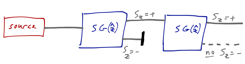
Since there are two discrete outputs from the \hat{z}-direction SG analyzer, we can label them as \ket{\uparrow} for S_z = +\hbar/2 and \ket{\downarrow} for S_z = -\hbar/2. (We could have used other labels, but the up/down arrow notation is fairly standard for two-state systems, so I’ll try to use it consistently.) Any input beam gives one of these two outputs, which means that we can write any state as a sum over them: \ket{\psi} = \alpha \ket{\uparrow} + \beta \ket{\downarrow} By the first postulate this state must be normalized, which means \left\langle \psi | \psi \right\rangle = |\alpha|^2 + |\beta|^2 = 1. We can also write \ket{\psi} as a column vector, which will be convenient: \ket{\psi} = \left( \begin{array}{c} \alpha \\ \beta \end{array} \right).
Alright, now that we know how to describe a physical state, what can we do with it?
All physical observables correspond to Hermitian operators.
When we pass our beam through the Stern-Gerlach analyzer, by splitting the beam, we can measure the spin S_z by simply looking at which of the two outputs the atoms come out of. This means that S_z is an observable - we can measure it! - so there is a corresponding Hermitian operator \hat{S_z}. (We’ll see exactly what it looks like below.)
Not all operators we will encounter are Hermitian, of course. In the context of the two-state system (of which S-G is a prototypical exampe), there is a pair of particularly useful operators \hat{S_+} = \ket{\uparrow} \bra{\downarrow} = \left( \begin{array}{cc} 0 & 1 \\ 0 & 0 \end{array} \right) \\ \hat{S_-} = \ket{\downarrow} \bra{\uparrow} = \left( \begin{array}{cc} 0 & 0 \\ 1 & 0 \end{array} \right).
These are called raising and lowering operators, respectively; the raising operator converts the state \ket{\downarrow} into \ket{\uparrow}, and vice-versa for the lowering operator. They are not Hermitian, and hence do not correspond to any physical observable; but they happen to be useful mathematical objects when studying with the two-state system, or especially when we return to spin and angular momentum in general.
When an observable \hat{A} is measured, the outcome is always an eigenvalue a of \hat{A}. After measurement, the state collapses into the corresponding eigenstate, \ket{\psi} \rightarrow \ket{a}.
The reason that we require Hermitian operators is because as we proved above, they have real eigenvalues, which (by postulate 3) correspond to the real numbers that come out of our experiments.
Coming back to \hat{S_z}, we know that there were two possible outcomes of the experiment, S_z = \pm \hbar/2, corresponding to the two eigenstates we’re using as our basis, \ket{\uparrow} and \ket{\downarrow}. In matrix form, then, we can write the corresponding operator as \hat{S_z} = \frac{\hbar}{2} \left( \begin{array}{cc} 1 & 0 \\ 0 & -1 \end{array} \right). Our chosen basis states \ket{\uparrow} and \ket{\downarrow} are the eigenvectors of this Hermitian operator; as a result, they form an orthonormal basis. Another way to see the structure of this matrix is to write it explicitly as a set of matrix elements: \hat{S_z} = \left( \begin{array}{cc} \bra{\uparrow} \hat{S_z} \ket{\uparrow} & \bra{\uparrow} \hat{S_z} \ket{\downarrow} \\ \bra{\downarrow} \hat{S_z} \ket{\uparrow} & \bra{\downarrow} \hat{S_z} \ket{\downarrow} \end{array} \right)
We know from experiment that if we begin with a pure output from a \hat{z}-direction analyzer, the next time we measure we’re guaranteed to get the same outcome, either \pm \hbar/2. Thus, the “collapse” of postulate 3 does nothing (if we’re already in an eigenstate), and we have \hat{S_z} \ket{\pm} = \pm \frac{\hbar}{2} \ket{\pm}. That gives the diagonal entries, and the orthogonality of eigenvectors \ket{\uparrow} and \ket{\downarrow} with each other gives the off-diagonal entries.
One important point was buried in that last argument: under certain circumstances, we were guaranteed to get a certain output. However, we know that quantum mechanics is probabilistic; for each individual atom passing through the \hat{S_z} measurement apparatus, we don’t generally know if we will record spin-up or spin-down. (Implicit in postulate 3 is the fact that we can’t predict which eigenvalue of \hat{A} will be measured as the outcome.) However, we can predict the probability of each measurement:
If a system is in state \ket{\psi}, then the probability of outcome \ket{a} from a measurement is \text{pr}(a) = |\left\langle a | \psi \right\rangle|^2.
As an important corrolary of Born’s rule, we should certainly insist that the total probability of all possible outcomes is equal to 1, or 1 = \sum_i |\left\langle a_i | \psi \right\rangle|^2 = \bra{\psi} \left( \sum_i \ket{a_i} \left\langle a_i | \psi \right\rangle \right) = \left\langle \psi | \psi \right\rangle. This is why we required that all physical states should be normalized above (or, if we don’t include it in postulate 1, we find that it is enforced on us here.)
If we repeat a measurement many times, the average value of the measurement is given by the expectation value: \left\langle \hat{A} \right\rangle = \sum_i \text{pr}(a_i) a_i \\ = \sum_i |\left\langle a_i | \psi \right\rangle|^2 a_i \\ = \sum_i \left\langle \psi | a_i \right\rangle a_i \left\langle a_i | \psi \right\rangle \\ = \sum_i \bra{\psi} \hat{A} \ket{a_i} \left\langle a_i | \psi \right\rangle \\ = \bra{\psi} \hat{A} \ket{\psi}. The spread in these measurements (the width of the distribution) is also interesting, and is determined by the variance \left\langle \hat{A}{}^2 \right\rangle - \left\langle \hat{A} \right\rangle{}^2, which we can evaluate similarly by sandwiching with the state vector \ket{\psi}.
The states of a quantum mechanical system evolve in time according to the Schrödinger equation, i\hbar \frac{\partial}{\partial t} \ket{\psi(t)} = \hat{H} \ket{\psi(t)},
where \hat{H} is the Hamiltonian operator.
For completeness, I am stating the time evolution postulate here, but we need to define the Hamiltonian operator to understand it. We will come back to this a little bit later. (The asterisk is due to some subtleties about how time evolution is defined, which again, we’ll come back to.)
Finally, some references include a sixth postulate known as the symmetrization postulate, which has to do with the behavior of identical particles, depending on whether they are fermions or bosons (which leads to famous results such as the Pauli exclusion principle.) We will come back to identical particles much later in the class. In my notes, I am not including this as a sixth postulate, because in relativistic quantum mechanics (i.e. quantum field theory), symmetrization can be derived from a deeper result known as the spin-statistics theorem.