15 Entanglement
Now we’re ready to tackle another important complication that lets us apply quantum mechanics to more realistic systems: extending our formalism to the presence of multiple particles at the same time. This will lead to all sorts of interesting quantum effects.
If we have two particles A and B, described independently by Hilbert spaces \mathcal{H}_A and \mathcal{H}_B, the obvious way to describe both at once is just to work in a combined space described by the direct product, \mathcal{H} = \mathcal{H}_A \otimes \mathcal{H}_B. This is indeed the correct way to construct a Hilbert space for our two-particle system, with a natural basis provided by the direct product as well, \ket{a_i} \otimes \ket{b_j}. However, several interesting complications will emerge from fleshing out the details of this basic idea. One of the more interesting complications starts with the simple observation that there exist many states within the space \mathcal{H}_A \otimes \mathcal{H}_B that cannot be described simply as a direct product of states taken from each space \ket{\psi_A} \otimes \ket{\psi_B}. These states are said to be entangled, or to exhibit entanglement.
A quantum state \ket{\psi} is said to be entangled if it is a state in a direct-product Hilbert space, e.g. \mathcal{H}_A \otimes \mathcal{H}_B, that cannot be written as a direct product of states from the individual Hilbert spaces,
\ket{\psi} \neq \ket{\psi_A} \otimes \ket{\psi_B}.
Let’s start with the simplest possible example: we take our two states to be spin-1/2 particles, so that each Hilbert space is two-dimensional, spanned by the spin states \ket{\uparrow} \equiv \ket{s=1/2, m=+1/2} and \ket{\downarrow} \equiv \ket{s=1/2, m=-1/2}. This means that our combined space is four dimensional, with basis \ket{\uparrow}_A \ket{\uparrow}_B, \ket{\uparrow}_A \ket{\downarrow}_B, \ket{\downarrow}_A \ket{\uparrow}_B, \ket{\downarrow}_A \ket{\downarrow}_B. (Direct products between the A and B states are implied from here on.) None of these states are entangled; by construction, they are all simple direct products. Other linear combinations of these states can be seen explicitly to not be entangled; for example, the combination \ket{\chi} = \frac{1}{\sqrt{2}} \left( \ket{\uparrow}_A \ket{\downarrow}_B + \ket{\downarrow}_A \ket{\downarrow}_B \right) can be factorized into \ket{\chi} = \frac{1}{\sqrt{2}} \left( \ket{\uparrow}_A + \ket{\downarrow}_A \right) \ket{\downarrow}_B = \ket{S_x = \uparrow}_A \ket{\downarrow}_B. However, there is a simple and famous state that is entangled: \ket{\psi_{EPR}} = \frac{1}{\sqrt{2}} \left( \ket{\uparrow}_A \ket{\downarrow}_B - \ket{\downarrow}_A \ket{\uparrow}_B \right). This is the EPR pair, named after a famous paper by Einstein, Podolsky, and Rosen which we’ll discuss below. This state is also known as a Bell state, after J.S. Bell, whose work we will also discuss below. This state cannot be written in any way as a direct product of states existing in the separate subspaces \mathcal{H}_A and \mathcal{H}_B. It is difficult to prove a negative, but we will see later explicit techniques that allow us to check whether a given quantum state is entangled or not.
Before we get to the formalism, an informal way to see if entanglement is present is to ask the question: if we make a measurement restricted only to subspace A, does the outcome of that measurement influence what happens when we subsequently make a measurement in subspace B? If the state has no entanglement, then by definition it can be factorized into some \ket{\phi}_A \otimes \ket{\psi}_B, which tells us that measurements on one space do not affect the other space; while a measurement will collapse \ket{\phi}_A to something, the part of the state living in the B subspace \ket{\psi}_B remains unaffected.
You can easily convince yourself that for the state \ket{\chi} above, the order of measurement (A first, or B first) doesn’t matter at all. On the contrary, it’s easy to see that if we measure \hat{S}_{z,A} on the EPR pair, as soon as we know the outcome, then the outcome of the corresponding \hat{S}_{z,B} measurement is guaranteed, since the remaining part of the EPR pair state is now an eigenstate of \hat{S}_{z,B}. This is the essence of entanglement.
Before we continue, let’s go back to our formalism for how measurements work, which so far has been a little too simplified to capture the physics we want to get into here.
15.1 Patching the measurement postulate
When we stated the measurement postulate way back at the beginning of these notes, we stated that after measurement, the state simply becomes the eigenstate corresponding to the measurement. However, now that we have two particles this doesn’t quite makes sense: we can’t say “the state \ket{\psi_{EPR}} collapses to \ket{\uparrow}_A”, because \ket{\uparrow}_A doesn’t live in the joint Hilbert space \mathcal{H}_A \otimes \mathcal{H}_B.
The more precise and general way to state the collapse part of the measurement postulate is as follows:
When an observable \hat{A} is measured, the outcome is always an eigenvalue a of \hat{A}. After measurement, the state is projected onto the corresponding subspace described by that eigenvalue,
\ket{\psi} \rightarrow \frac{1}{\sqrt{\bra{\psi} \hat{P}_a \ket{\psi}}} \hat{P}_a \ket{\psi},
where we divide by the additional factor \sqrt{\bra{\psi} \hat{P}_a \ket{\psi}} to maintain the normalization of the state. This is known as a projective measurement. Note that by Born’s rule, \bra{\psi} \hat{P}_a \ket{\psi} = p(a), the probability of measuring outcome a.
This version of the postulate uses the idea of a projection operator, \hat{P}_a, which we need to define. If the eigenvalue a corresponds to a unique single state \ket{a}, then the projection operator is simply the outer product of that state with itself:
\hat{P}_a = \ket{a}\bra{a}, and we recover the simpler version of the measurement postulate with collapse to a single state.
The situation changes if there is degeneracy, meaning that there are multiple eigenstates with the same eigenvalue. In this case, instead of just a single state there is a degenerate subspace of dimension greater than 1 corresponding to such an eigenvalue. The projection operator then maps us into that subspace: \hat{P}_a = \sum_{i=1}^N \ket{a}_i \bra{a}_i, where the size of the subspace is N, and the \ket{a}_i are a set of N orthonormal basis vectors that we’ve chosen to span this subspace. This basis is not uniquely determined by the eigenvector problem, since linear combinations of \ket{a}_i are still eigenvectors of \hat{A}. Even so, the state we get after projecting is still unique - it doesn’t depend on how we choose our basis (indeed, we already think of a general quantum state \ket{\psi} as something that exists independent of basis choice.)
In our previous discussions, particularly relating to complete sets of commuting operators (CSCOs), we noted that the presence of degeneracy often signals that there is some additional measurement we can do to break the degeneracy. However, even if we know a CSCO for a given system we’re not always necessarily taking all possible measurements at once, and that means that we can end up measuring quantities that don’t completely fix the quantum state to a single basis vector. A CSCO just tells us that we can perform a series of measurements that will collapse our state to a single basis ket.
We’ve encountered a few cases with degeneracies in previous chapters, but now that we’re interested in multi-particle systems degeneracies are much more common. In fact, this is directly relevant for the case we were just discussing with the EPR pair and “measurement on spin A”. If we measure \hat{S}_{z,A}, the complete measurement operator on the joint Hilbert space is in fact \hat{S}_{z,A} \otimes \hat{1}_B, that is, it is combined with the identity operator for spin B - which is always very degenerate, since all states have eigenvalue 1 for the identity.
15.1.1 Example - degenerate measurement in two-spin system
Consider a pair of spins with s=1/2, labelled \hat{\vec{S}}_A and \hat{\vec{S}}_B. We measure the total spin-squared operator \hat{\vec{S}}^2, where \hat{\vec{S}} = \hat{\vec{S}}_A + \hat{\vec{S}}_B. In the product basis \ket{m_1 m_2}, the four basis states are \ket{\uparrow \uparrow}, \ket{\uparrow \downarrow}, \ket{\downarrow \uparrow}, \ket{\downarrow \downarrow} while we know that our measurement is best described in the total basis \ket{s,m}, with \ket{1,1} = \ket{\uparrow \uparrow} \\ \ket{1,0} = \frac{1}{\sqrt{2}} (\ket{\uparrow \downarrow} + \ket{\downarrow \uparrow}) \\ \ket{1,-1} = \ket{\downarrow \downarrow} \\ \ket{0,0} = \frac{1}{\sqrt{2}} (\ket{\uparrow \downarrow} - \ket{\downarrow \uparrow}).
The two possible measurement outcomes for \hat{\vec{S}}^2 are s=0 or s=1, either one giving \hbar^2 s(s+1) - but we’re more interested in the eigenvalue s itself. If the measurement outcome is s=0, then there is no degeneracy and any quantum state will collapse into \ket{0,0}: s=0 \Rightarrow \ket{\psi} \rightarrow \ket{0,0} = \frac{1}{\sqrt{2}} (\ket{\uparrow \downarrow} - \ket{\downarrow \uparrow}). (By the way, the \ket{0,0} state is precisely the EPR state we just introduced, so here is a concrete way to prepare such a state for a pair of spin-1/2s!) On the other hand, if we measure s=1 then there is a three-way degeneracy. Since we’ve already built a basis, the corresponding projection operator is simply the sum over the individual projectors for each basis vector: \hat{P}_{s=1} = \ket{1,1}\bra{1,1} + \ket{1,0}\bra{1,0} + \ket{1,-1}\bra{1,-1}, and then s=1 \Rightarrow \ket{\psi} \rightarrow \frac{1}{\sqrt{p(s=1)}} \hat{P}_{s=1} \ket{\psi}.
With all of that set up, let’s think about a couple of measurements and how things will collapse afterwards. There are lots of simple examples: for example, if our initial state is \ket{\psi_0} = \ket{\uparrow \downarrow} = \frac{1}{\sqrt{2}} (\ket{1,0} + \ket{0,0}), then measuring \left\langle \hat{\vec{S}^2} \right\rangle will give us either s=0 or s=1 with 50% probability, collapsing the state into either \ket{0,0} or \ket{1,0}. Applying the projector explicitly, we have s=1 \Rightarrow \ket{\psi_0} \rightarrow \frac{1}{\sqrt{1/2}} \left( \ket{1,1} \left\langle 1,1 | \psi_0 \right\rangle + \ket{1,0} \left\langle 1,0 | \psi_0 \right\rangle + \ket{1,-1} \left\langle 1,-1 | \psi_0 \right\rangle \right) \\ = \sqrt{2} \left( \frac{1}{\sqrt{2}} \ket{1,0} \right) = \ket{1,0}.
A more interesting example is the state \ket{\psi_1} = \frac{1}{\sqrt{2}} \left(\ket{\uparrow \downarrow} + \ket{\downarrow \downarrow} \right) \\ = \frac{1}{2} \left( \ket{1,0} + \ket{0,0} + \sqrt{2} \ket{1,-1} \right).
Now the projector onto the s=1 subspace gives us \hat{P}_{s=1} \ket{\psi_1} = \frac{1}{2} \ket{1,0} + \frac{1}{\sqrt{2}} \ket{1,-1}, with a corresponding measurement probability of p(s=1) = \bra{\psi_1} \hat{P}_{s=1} \ket{\psi_1} = \frac{1}{4} \left\langle 1,0 | 1,0 \right\rangle + \frac{1}{2} \left\langle 1,-1 | 1,-1 \right\rangle = \frac{3}{4}. The leftover state after such a measurement will be \ket{\psi'_1} = \frac{1}{\sqrt{p(s=1)}} \hat{P}_{s=1} \ket{\psi_1} = \frac{1}{\sqrt{3}} \ket{1,0} + \sqrt{\frac{2}{3}} \ket{1,-1}. Mechanically, we can see that all our measurement is doing is picking out the s=1 states in the collapse and then normalizing the result. This preserves the relative weight of \ket{1,0} versus \ket{1,-1} from the initial state.
15.2 The EPR “paradox”
There is a deeply concerning fact for any physicist lurking in the details of our statements about measurement and entangled states, even in the very simple spin-1/2 system we’ve been thinking about. This fact is the basis of the 1935 paper by Einstein, Podolsky and Rosen after which the EPR state is named. This fact is also so simple that we don’t need any sophisticated arguments to be concerned. Here is the EPR state once again: \ket{\psi_{EPR}} = \frac{1}{\sqrt{2}} \left( \ket{\uparrow}_A \ket{\downarrow}_B - \ket{\downarrow}_A \ket{\uparrow}_B \right).
As we noted above, a characteristic feature of entanglement in the EPR state is that once we measure \hat{S}_{z,A}, the outcome of measuring \hat{S}_{z,B} is fully determined. But this statement is independent of the details of our experiment. So now we imagine two experimenters, Alice with spin A and Bob with spin B (following the standard quantum information naming conventions), who take the spins and to their own separate labs that are separated by a large distance. Now Alice makes a measurement of the z-direction spin; let’s say that she obtains \ket{\uparrow}_A as the result. What does Bob see when he measures the z component of his own spin? Well, after Alice’s measurement the state collapses by projection onto \ket{\psi_{EPR}} \rightarrow \ket{\uparrow}_A \ket{\downarrow}_B, so Bob has a 100% chance of measuring the outcome \ket{\downarrow}_B.
Now here is the problem: once Alice has made her measurement, the outcome of Bob’s experiment is known before he measures his system, no matter how far away he is, and no matter how quickly he measures - even if the measurement is done before a signal arrives from Alice’s lab at the speed of light to tell him the result of her experiment.
This very simple observation is sometimes breathlessly presented at this point as a violation of locality, since some kind of “signal” appears to be propagating faster than light. However, it’s important to realize that there isn’t actually any way of transferring information faster than light in this example, because Alice doesn’t have any control over the outcome of her spin measurement, and on the other side Bob has no way of telling from the outcome of his measurement whether Alice has actually collapsed the state or not. If they meet up and share a sequence of EPR pairs, then go to their separate labs and take measurements, in isolation either chain of measurements just looks purely random:
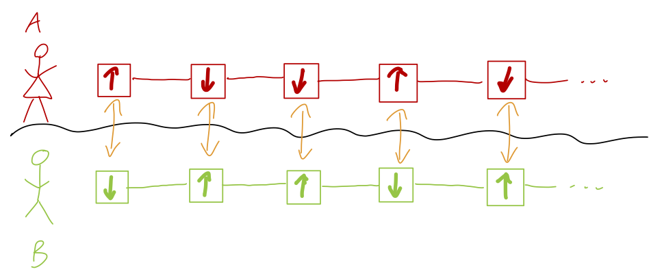
The perfect anti-correlation of outcomes is only revealed when they meet up and compare notes on their measurement results. The only thing that is propagating faster than light (if their labs are far enough apart) is the collapse of the state of each pair due to the measurement.
Of course, this assumes that collapse requires some form of “propagation” between distant parts of an entangled state. There is another possibility, which can be illustrated with a simple classical example. Suppose that I have a matching pair of salt and pepper shakers, and when Alice and Bob meet to share their EPR-pair spins, I give them each a sealed box containing one of the shakers. When Alice gets to her lab, if she opens the box and finds my pepper shaker, then she immediately knows that Bob has the salt shaker. But nothing mysterious or non-local is happening: this is just a classical correlation that was fixed when I gave them the two boxes before they were separated. In the classical example, “measurement” just amounts to revealing hidden information that was there the whole time.
The key difference in this example is that there is a hidden variable which is set in a perfectly local way: the information as to whether I put the salt shaker into Alice’s box, or not. Even if I blindfold myself before sealing the shakers in the two boxes, so nobody knows which is which until they are opened, we still believe in a model of reality in which the salt shaker is either in Alice’s box or not; the outcome is determined at the moment I seal them.
This brings us to the EPR “paradox”, where I put paradox in quotes because it’s not really a paradox, at least the way I am presenting the argument. In quantum mechanics, the state vector \ket{\psi_{EPR}} seems not to contain enough information to tell us the outcome of the experiment; we only know the probability of each outcome. This means that if quantum reality is like the salt and pepper shakers, we have to extend quantum mechanics by adding some hidden variables that pre-determine the outcome of the measurement before Alice and Bob split their entangled spins apart. The only apparent alternative is non-locality, that is, that there is some phenomenon of collapsing due to measurement that can travel arbitrarily fast.
I should stress that the idea of “hidden variables”, which goes by the name of local realism, does not mean that we suddenly have a deterministic theory of nature. We certainly know from experiment that the world on quantum scales is inherently probabilistic. But probability famously comes from lack of knowledge: every elementary probability class begins with something like taking a bag of red and blue balls and mixing them up before drawing one at random; we can’t predict exactly which color of ball we will pull next because that knowledge has been scrambled away. But we believe that each ball in the bag can still be labeled as “red” or “blue”, even if we’re not looking at them.
Similarly, perhaps each of our spins in this quantum system has a secret label s_z = \pm 1 that determines what the outcome of the \hat{S}_z measurement is going to be. We can assume these variables are perfectly hidden by Nature, so that there is no way we can ever access them directly; when we split the EPR pair apart we know one has s_z = +1 and one has s_z = -1, but we have no way to tell which is which until we do our measurement. This is a perfectly good theory to describe the situation where Alice and Bob only ever do measurements in the z direction; there is no funny faster-than-light propagation of anything.
In short, it seems that we either have to give up locality, or we have to give up our current formulation of quantum mechanics. The simple measurement of \hat{S}_{z,A} and \hat{S}_{z,B} can’t help us distinguish between these two, but it turns out that we can gain more information by considering some additional measurement options. After all, the classical example of correlations we’re using as an analogy relies on the classical rules of probability, but as we learned at the very beginning of this class, interference effects that force us to extend our understanding of probabilities are really the essence of quantum mechanics.
15.3 Bell inequalities
The key to unraveling this mystery is in the fact that the spin-singlet state \frac{1}{\sqrt{2}} (\ket{\uparrow} - \ket{\downarrow}) contains more information than just telling us we have a 50-50 probability of measuring either spin-up or spin-down in the z direction. It also encodes the probabilities for measuring the spin in any direction at all.
To set things up, let’s consider the possibility of measuring the spin along an arbitrary axis, \vec{n}. Using spherical coordinates, the unit vector pointing along an arbitrary axis can be written as \vec{n} = (\sin \theta \cos \phi, \sin \theta \sin \phi, \cos \theta) which means that \hat{\vec{\sigma}} \cdot \vec{n} can be simplified to, working in the spin-z basis, \hat{\vec{\sigma}} \cdot \vec{n} = \left(\begin{array}{cc} \cos \theta & e^{-i\phi} \sin \theta \\ e^{i\phi} \sin \theta & -\cos \theta \end{array} \right). The eigenvalues should still be \pm 1, since in another coordinate system this is just \hat{\sigma}_{z'}; it’s easy to check that the corresponding eigenkets are \ket{n_\uparrow} = e^{-i\phi} \cos(\theta/2) \ket{\uparrow} + \sin(\theta/2) \ket{\downarrow} \\ \ket{n_\downarrow} = -e^{-i\phi} \sin(\theta/2) \ket{\uparrow} + \cos(\theta/2) \ket{\downarrow} \\
Now knowing the eigenstates, we can rewrite the EPR state in the basis given by n-axis measurements. The result is very simple: \ket{\psi_{EPR}} = \frac{1}{\sqrt{2}} \left( \ket{n_\uparrow}_A \ket{n_{\downarrow}}_B - \ket{n_\downarrow}_A \ket{n_\uparrow}_B \right). (This might be surprising but it’s just a consequence of rotational invariance, actually; as we know the EPR state is the \ket{s,m} = \ket{0,0} state in the total spin basis, which means that it is completely invariant under rotations, in the sense that we can pick any direction we want as the z axis and the state is written the same way.)
15.3.1 Measurements along two different axes
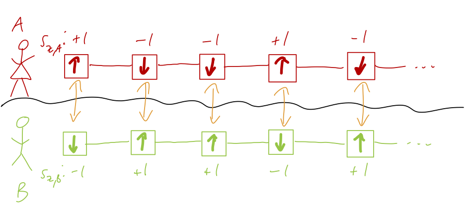
Now let’s start digging in to probabilities, starting with the simplest case where both Alice and Bob measure along the same axis, call it the z axis. There are four possibilities to enumerate, using Born’s rule: p_{QM}(\uparrow_{z,A}, \uparrow_{z,B}) = 0 \\ p_{QM}(\uparrow_{z,A}, \downarrow_{z,B}) = 1/2 \\ p_{QM}(\downarrow_{z,A}, \uparrow_{z,B}) = 1/2 \\ p_{QM}(\downarrow_{z,A}, \downarrow_{z,B}) = 0. Here p_{QM} denotes the probability of each outcome as predicted by quantum mechanics. This is trivially reproduced by a hidden-variable theory: we just postulate two hidden variables s_{z,A/B} and then assign p(s_{z,A} = +1, s_{z,B} = -1) = p(s_{z,A} = -1, s_{z,B} = +1) = 1/2, and then for example p_{HV}(\uparrow_{z,A}, \downarrow_{z,B}) = p(s_{z,A} = +1, s_{z,B} = -1) = 1/2, predicting all the same results as the quantum mechanical theory. Note that there is nothing non-local happening here, even though this is a probability distribution relating properties of Alice’s spins and Bob’s spins; these are just classical probability correlations, exactly the same as the anti-correlation when I randomly split my salt and pepper shaker apart.
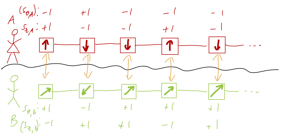
Now let’s suppose that they choose different axes to measure along. Without loss of generality, let’s take Alice’s choice to be the z axis, while Bob measures on an axis \vec{n} which is rotated by \theta, with \phi = 0. Following Born’s rule again, we have p_{QM}(\uparrow_{z,A}, \uparrow_{\theta,B}) = \left|(\bra{\uparrow}_A \otimes \bra{n_{\uparrow}}_B) \ket{\psi_{EPR}} \right|^2 \\ = \left| \frac{-1}{\sqrt{2}} \bra{\uparrow}_A \ket{n_\downarrow}_A \right|^2 \\ = \frac{1}{2} \sin^2 \left( \frac{\theta}{2} \right). The other three possibilities are easily computed to be p_{QM}(\uparrow_{z,A}, \downarrow_{\theta,B}) = \tfrac{1}{2} \cos^2 (\theta/2) \\ p_{QM}(\downarrow_{z,A}, \uparrow_{\theta,B}) = \tfrac{1}{2} \cos^2 (\theta/2) \\ p_{QM}(\downarrow_{z,A}, \downarrow_{\theta,B}) = \tfrac{1}{2} \sin^2 (\theta/2). \\
Going back to the hidden-variable description, now we have to assign a second hidden variable for each spin to deal with the \vec{n} axis: let’s call it s_{\theta}. We know that if Alice and Bob were to measure on the same axis they would get the simple results from above, which tells us that p(s_{\theta,A} = +1, s_{\theta,B} = -1) = p(s_{\theta,A} = -1, s_{\theta,B} = +1) = 1/2. We are still free to specify the joint probability distributions between s_z and s_\theta, and we simply match on to the QM predictions once again: p(s_{z,A} = +1, s_{\theta,B} = +1) = p(s_{z,A} = -1, s_{\theta,B} = -1) = \tfrac{1}{2} \sin^2 (\theta/2), \\ p(s_{z,A} = +1, s_{\theta,B} = -1) = p(s_{z,A} = -1, s_{\theta,B} = +1) = \tfrac{1}{2} \cos^2 (\theta/2). and p_{HV}(...) is specified from the corresponding hidden-variable probabilities.
So far this all feels kind of trivial, but there is a key difference between the QM and HV descriptions, which is that there is a classical probability distribution that describes the hidden variables, while in quantum mechanics we only have probability amplitudes. This means that secretly, there is a probability distribution function in terms of all four hidden variables at once (either experimenter can measure on either axis): p(s_{z,A} = \pm 1, s_{\theta,A} = \pm 1, s_{z,B} = \pm 1, s_{\theta,B} = \pm 1) = ... This must exist since by definition, all four hidden variables exist at once: for example, if Alice measures on the z axis and Bob on the \vec{n} axis, their measurement outcomes fix the corresponding hidden variables for both spins due to perfect anti-correlation.
Classical probabilities obey certain rules, such as marginalization: we know that in general, \sum_B p(A,B) = p(A).
This can be used to make simple statements about how certain probabilities are related. For example, we have p(s_{z,A} = +1, s_{\theta,B} = +1) + p(s_{z,A} = +1, s_{\theta,B} = -1) = p(s_{z,A} = +1). We know the probability on the right-hand side has to just be 1/2, since that’s the probability in isolation that Alice will measure the result \uparrow_{z,A}, and because the hidden-variable theory is local this can’t depend on anything that Bob does if they are spatially separated. Plugging in on the left-hand side, \frac{1}{2} \sin^2 (\theta/2) + \frac{1}{2} \cos^2 (\theta/2) = 1/2 and everything looks good. This particular marginalization statement is true in both the HV and QM theories, since it only involves experimental probabilities that we can measure.
Let’s explore a bit more what the full hidden-variable probability distribution has to look like. At first glance it seems like we need to specify 16 numbers in total to fully define it. But the requirement of perfect anti-correlation of the outcomes means that in any case where Alice and Bob could measure on the same axis and get the same outcome, the corresponding probability is zero, for example p(s_{z,A} = +1, s_{\theta,A} = +1, s_{z,B} = +1, s_{\theta,B} = -1) = 0 since we can never have s_{z,A} = s_{z,B} = +1. This means that there are only a few probabilities that are non-zero in the full hidden probability distribution, and they’re all given in terms of the results we’ve computed above.
We could go through and fully enumerate the entire hidden distribution, but we don’t need to do that to make one more very interesting observation. The property of marginalization, together with the observation that s_{n,A} = s_{n,B} results in zero probability, lets us actually write down a joint probability between just Alice’s hidden variables: p(s_{z,A} = +1, s_{\theta,A} = +1) = p(s_{z,A} = +1, s_{\theta,A} = +1, s_{z,B} = -1, s_{\theta,B} = -1) \\ = p(s_{z,A} = +1, s_{\theta,B} = -1) = \tfrac{1}{2} \cos^2 (\theta/2). This is an example of a counterfactual probability, because it relates two hidden variables that describe mutually exclusive experiments: Alice measuring on the z axis and on the rotated n axis. We cannot access this probability directly from experiment; it tells us something about what the outcomes would be if we could measure along z, and then go back and measure along \theta. In quantum mechanics, there is no way to predict this probability, but it is perfectly well-defined in the hidden variables theory.
While the existence of this counterfactual probability is a difference between quantum mechanics and hidden variables, it’s also not something we can ever access in experiment, so it isn’t a discrepancy we can test. But something interesting will happen if we allow for one more measurement.
15.3.2 Measurements along three different axes
Let’s consider a second possible axis n', which has the same \theta as axis n but now has a non-zero polar angle \phi. What are the measurement probabilities now? Starting in quantum mechanics, if Alice uses the z axis and Bob uses the n' axis, the phase is irrelevant and the outcome is the same: p_{QM}(\uparrow_{z,A}, \uparrow_{\phi,B}) = \frac{1}{2} \sin^2 \left( \frac{\theta}{2} \right) and so on. The new results occur when Alice uses the n axis. After some algebra and trig identities, we find the results p_{QM}(\uparrow_{\theta,A}, \downarrow_{\phi,B}) = |(\bra{n_\uparrow}_A \otimes \bra{n'_\downarrow}_B) \ket{\psi_{EPR}}|^2 \\ = \frac{1}{2} \left( 1 - \sin^2 (\phi/2) \sin^2 \theta \right), and p_{QM}(\uparrow_{\theta,A}, \uparrow_{\phi,B}) = \frac{1}{2} \sin^2 \theta \sin^2(\phi/2). Notice that we have as a check the marginalization condition p_{QM}(\uparrow_{\theta,A}) = p_{QM}(\uparrow_{\theta,A}, \uparrow_{\phi,B}) + p_{QM}(\uparrow_{\theta,A}, \downarrow_{\phi,B}) \\ = \frac{1}{2} \sin^2 \theta \sin^2(\phi/2) + \frac{1}{2} (1 - \sin^2 \theta \sin^2 (\phi/2)) = \frac{1}{2}, as it should.
Do the algebra out and show the two results for joint measurement probabilities given above.
Answer:
Starting with the first case, p_{QM}(\uparrow_{\theta,A}, \downarrow_{\phi,B}) = |(\bra{n_\uparrow}_A \otimes \bra{n'_\downarrow}_B) \ket{\psi_{EPR}}|^2 \\ = \frac{1}{2} \left| (\bra{n_\uparrow}_A) (\ket{n'_\uparrow}_A) \right|^2 \\ = \frac{1}{2} \left| e^{-i\phi} \cos^2 \left( \frac{\theta}{2} \right) + \sin^2 \left( \frac{\theta}{2} \right) \right|^2 \\ = \frac{1}{2} \left( \cos^4 (\theta/2) + \sin^4 (\theta/2) + 2 \cos \phi \sin^2 (\theta/2) \cos^2 (\theta/2) \right) \\ = \frac{1}{2} \left( 1 - 2 \sin^2 (\theta/2) \cos^2 (\theta/2) + 2 \cos \phi \sin^2 (\theta/2) \cos^2 (\theta/2) \right) \\ = \frac{1}{2} \left( 1 - \frac{1}{2} (1 - \cos \phi) \sin^2 \theta \right) \\ = \frac{1}{2} \left( 1 - \sin^2 (\phi/2) \sin^2 \theta \right).
Now the second probability: p_{QM}(\uparrow_{\theta,A}, \uparrow_{\phi,B}) = |(\bra{n_\uparrow}_A \otimes \bra{n'_\uparrow}_B) \ket{\psi_{EPR}}|^2 \\ = \frac{1}{2} \left| (\bra{n_\uparrow}_A) (\ket{n'_\downarrow}_A) \right|^2 \\ = \frac{1}{2} \left| -e^{-i\phi} \cos (\theta/2) \sin (\theta/2) + \cos (\theta/2) \sin (\theta/2) \right|^2 \\ = \frac{1}{2} \sin^2 (\theta/2) \cos^2 (\theta/2) (4 \sin^2 (\phi/2)) \\ = \frac{1}{2} \sin^2 \theta \sin^2(\phi/2).
If we go on to calculate the other two probabilities, we’ll find that p_{QM}(\downarrow_{\theta,A}, \uparrow_{\phi,B}) = \frac{1}{2} (1 - \sin^2 \theta \sin^2 (\phi/2)), \\ p_{QM}(\downarrow_{\theta,A}, \downarrow_{\phi,B}) = \frac{1}{2} \sin^2 \theta \sin^2 (\phi/2), which we can also obtain by the shortcut of just imposing marginalization using the two results we already calculated.
Now, back to our hidden-variable theory again. Since we have a new measurement axis, we once again have to assign a new hidden variable s_\phi that will label the spin outcomes along the n' axis. We must have a different variable for this new axis, since it has to be set locally when the spins are separated, long before Bob decides which axis to measure along. The joint probability distributions for the paired s_{z,A}, s_{\phi,B} measurements are the same, e.g. p(s_{\theta,A} = +1, s_{\phi,B} = +1) = \tfrac{1}{2} \sin^2 (\phi/2) \sin^2 \theta and so on.
Now we come to the crux of the argument: the hidden-variable model says that all of s_z, s_\theta, s_\phi are hidden properties of our spin that exist simultaneously. This means that there exists a joint probability distribution between all three hidden variables at once: p(s_{z,A/B} = \pm 1, s_{\theta,A/B} = \pm 1, s_{\phi,A/B} = \pm 1) = p(\pm_{z,A/B}, \pm_{\theta,A/B}, \pm_{\phi,A/B}) = ... introducing some shorthand since the notation is getting a little unwieldy with three variables. We can never access this probability function directly, since we have only two spins and two measurements we can do, but nevertheless in the hidden-variable model it has to exist - and that is all we need in order to say something interesting. By the rules of probability, we can write the following two-measurement probabilities by marginalizing over the third measurement: p(+_{\theta,A}, -_{\phi,B}) = p(+_{z,A}, +_{\theta,A}, -_{\phi,B}) + p(-_{z,A}, +_{\theta,A}, -_{\phi,B}) \\ p(+_{z,A}, +_{\theta,A}) = p(+_{z,A}, +_{\theta,A}, +_{\phi,B}) + p(+_{z,A}, +_{\theta,A}, -_{\phi,B}) \\ p(-_{z,A}, -_{\phi,B}) = p(-_{z,A}, +_{\theta,A}, -_{\phi,B}) + p(-_{z,A}, -_{\theta,A}, -_{\phi,B}). Now, if we add the last two equations together, on the right-hand side we get the first line plus two terms which are probabilities and therefore positive. This gives us an inequality: p(+_{\theta,A}, -_{\phi,B}) \leq p(+_{z,A}, +_{\theta,A}) + p(-_{z,A}, -_{\phi,B}) But we know all three of these probabilities already:
1 - \sin^2 \left( \frac{\phi}{2} \right) \sin^2 \theta \leq 2 \cos^2 \left( \frac{\theta}{2} \right). This, finally, is a Bell inequality, named after J.S. Bell and his groundbreaking paper on testing the EPR paradox. It must be satisfied by a hidden-variable model that reproduces the results of our simple quantum mechanical spin measurements; it follows from simple manipulations based on the rules of probability, without even needing specify the full joint probability distribution of our hidden variables. And if we allow any possible \theta and \phi, the inequality simply fails to be satisfied. For example, the choices \theta = 3\pi/4 and \phi = \pi/2 give the result
1 - \left(\frac{1}{2}\right) \left( \frac{1}{2} \right) \leq 2 \cos^2 \left( \frac{3\pi}{8} \right) \Rightarrow \frac{3}{4} \leq 0.292 which is obviously false. We can make a numerical plot to see the entire range of values where the inequality is violated:
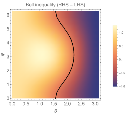
The black line shows where the inequality becomes an equality; to the right of it, the Bell inequality is violated, for a large part of the parameter space (generally with fairly large angles between the axes.)
15.3.3 Implications of the Bell inequality
At this point, we have an experimental way to distinguish whether hidden variables and local reality are present, or not. What the Bell inequality tells us is that for certain choices of measurement angles, the predictions of the hidden variable theory - as we have defined it to perfectly match the predictions of quantum mechanics - are not self-consistent. This leaves two possibilities, if we measure using a set of axes for which the Bell inequality would be violated: either we get back the quantum-mechanical prediction, at which point the hidden variable theory must be discarded; or we find a deviation from quantum mechanics as we’ve written it, and maybe reality is in fact described by a local hidden-variables theory.
Many experimental tests of systems that satisfy Bell inequalities (“Bell tests”) have been carried out since the 1980s, with the groundbreaking result by Aspect, Grangier and Roger in 1982 viewed as the first decisive test. The result is that the Bell inequalities are indeed violated experimentally; the quantum mechanical description is the one that works.
Since our attempt to preserve local reality (hidden variables) has failed, there is a popular misconception that the Bell tests establish that there is truly something non-local happening - Einstein’s “spooky action-at-a-distance”. But in the example above, there was no experimental violation of locality and no way to send any information faster than light - and none of the other more complicated Bell tests show any such locality violation, either.
What the loss of hidden variables does require us to give up (up to much weirder modifications that amount to loopholes) is the idea of counterfactual definiteness, which is the notion that we can say what could have happened if we had run an experiment differently. This was a key ingredient in our study above: the Bell inequality relied on calculating the probability distribution p(+_{z,A}, +_{\theta,A}). This is inherently counterfactual, since it describes two different measurements applied to the same initial entangled state - but in quantum mechanics we can only choose to do one measurement, and then the state has collapsed.
To put this in more experimental terms, suppose that Alice measures along the z axis and Bob measures along the n axis. In the hidden variable theory, the perfect anti-correlation of measurements along the same axis tells Bob that if Alice had chosen to measure along n as well, she would have measured the opposite of whatever he saw. This defines the distribution above - but this is exactly what led to the Bell inequality, which is violated. Quantum mechanics instead says that we can’t make such a counterfactual statement; Bob’s measurement outcome only allows him to predict with what probability Alice will see specific outcomes, depending on how she measures (or has measured, since the order in time doesn’t matter).
The take-away message of all this is that our description of quantum measurement and state collapse isn’t non-local, it’s just deeply against our classical intuition. Collapse is more of a representation of how the information (or uncertainty) contained in our quantum state is altered when we take a measurement; ultimately, the relationship between Alice’s and Bob’s measurements is just a fancy quantum version of the simpler classical correlation when I separate my salt and pepper shaker and give one to each.
There are many other variations on the theme of devising quantum systems in which quantum mechanics predicts a certain set of possible outcomes which are not achievable within a hidden-variable version of the theory. One of the more famous examples is the CHSH (Clauser-Horne-Shimony-Holt) inequality, which I won’t discuss here but should be easy for you to find in other notes.
Another Bell test in a different setup is due to Greenberger, Horne, and Zeilinger (GHZ), involving the so-called “GHZ state”, \ket{\psi_{GHZ}} = \frac{1}{\sqrt{2}} (\ket{\uparrow \uparrow \uparrow} + \ket{\downarrow \downarrow \downarrow}). This is a similar test, but interesting because it involves more than two entangled particles at once. The GHZ state is part of a class of quantum states known as “cat states”, so-called because they are superpositions of two states in which all spins take on one maximal value or another - just like Schrödinger’s cat being in a superposition of the “alive” and “dead” states in the famous thought experiment.
15.4 Qubits and quantum communication
You have probably heard the term qubit before, short for “quantum bit”. A bit is the basic unit of information in a binary computer: a value b which can take on either the value 0 or 1. Any message or other piece of information can be encoded in some number of bits (a single character in ASCII encoding requires 7 bits, for example.) A bit is sort of a classical two-state system, so the analogous thing to do in quantum mechanics is also a two-state system. An arbitrary qubit, then, can be written as \ket{\chi} = c_0 \ket{0} + c_1 \ket{1}. As we’ve already studied the Bloch-sphere representation, we know that two real numbers are required to describe an arbitrary \ket{\chi}, with the other two apparent real degrees of freedom removed by normalization and global phase rotation.
Naively, it seems like our quantum bit has infinitely more capacity for information than a classical bit; the classical bit can take on only two discrete values, but the qubit encodes two real numbers, a continuous range of possibilities! Unfortunately, we have no practical access to these two real numbers. We know that any possible measurement on this system will have a binary outcome, e.g. either \uparrow or \downarrow if it’s a spin system and we measure along some chosen axis. As soon as we take such a measurement, the state collapses, so no matter what the qubit \ket{\chi} only encodes a single bit of accessible classical information. There is a result known as Holevo’s theorem which provides a more rigorous version of this statement: from a set of n qubits, we cannot send any more than n classical bits of information.
(We could, perhaps, manufacture a huge number of identical \ket{\chi} states from some process, and then making a large number of measurements might allow us to reconstruct c_0 or c_1. But the inherent randomness of quantum measurement means that we can only do this with some uncertainty; and anyway, at this point we’re using a huge number of qubits, whereas there are already better ways of encoding real numbers using large numbers of ordinary classical bits.)
The fact that there seems to be more information in a qubit until we have to read it out suggests that the bottleneck is more in the classical read-out part. Indeed, the entire premise of the field of quantum computing is that we can exploit entanglement and interference to do certain types of calculations with great efficiency. There is no contradiction, since we are relying on the quantum nature of the internal states for the algorithm we run on our quantum computer. Only when we read out the information at the end are we restricted by Holevo’s theorem.
We can get a taste of some of the novel applications enabled by using qubits with a couple of simple examples, once again relying heavily on entanglement in the form of the EPR state.
15.4.1 Superdense coding
Once again, let’s return to our two experimenters Alice and Bob, and suppose they have two qubits A,B available between them. Here is a simple encoding that will allow Alice to send a message to Bob:
Alice prepares the quantum state by placing each spin in an eigenstate of \hat{S}_z, with \uparrow used to encode 1 and \downarrow for 0. For example, if she prepares the state \ket{\chi_{01}} = \ket{\downarrow}_A \ket{\uparrow}_B, this represents the classical pair of bits 01.
Alice sends her quantum state to Bob, and tells him to also measure both qubits along the z axis. He reads the outcome and obtains the classical information. If she gives him the state \ket{\chi_{01}}, he finds the outcome \downarrow_{z,A}, \uparrow_{z,B} and infers “01” as the message.
This protocol uses two qubits to send two classical bits; due to Holevo’s theorem, we already know this is the best we can do (and this seems much harder than just writing down “01” on a piece of paper!) Although we can’t increase the total size of the message using qubits, there is another protocol which allows us to send that information in a very different way.
Alice prepares the qubits in an EPR pair state, \ket{\psi_{EPR}} = \frac{1}{\sqrt{2}} (\ket{\uparrow}_A \ket{\downarrow}_B - \ket{\downarrow}_A \ket{\uparrow}_B), and she gives spin B to Bob.
Later on, Alice does a quantum operation on her spin A, which takes the form of a two-by-two matrix \hat{O}_A. This only changes the state of her own qubit, but the entanglement with spin B is unaffected. For example, she could act with each of the Pauli matrices: \ket{\psi_x} = \hat{\sigma}_{x,A} \ket{\psi_{EPR}} \\ = \left( \begin{array}{cc} 0 & 1 \\ 1 & 0 \end{array} \right)_A \ket{\psi_{EPR}} \\ = \frac{1}{\sqrt{2}} (\ket{\downarrow}_A \ket{\downarrow}_B - \ket{\uparrow}_A \ket{\uparrow}_B). Moving on to the other two, \ket{\psi_y} = \hat{\sigma}_{y,A} \ket{\psi_{EPR}} = \frac{i}{\sqrt{2}} (\ket{\downarrow}_A \ket{\downarrow}_B + \ket{\uparrow}_A \ket{\uparrow}_B), \\ \ket{\psi_z} = \hat{\sigma}_{z,A} \ket{\psi_{EPR}} = \frac{1}{\sqrt{2}} (\ket{\uparrow}_A \ket{\downarrow}_B + \ket{\downarrow}_A \ket{\uparrow}_B). Her fourth choice is to do nothing (i.e. \hat{O}_A = \hat{1}, the identity.) All four of the states she can produce are orthogonal to one another.
After acting on her own qubit, she sends it to Bob, so that he now has the full entangled two-qubit state. Then Bob makes a measurement in order to decode the message. To avoid losing the message, he needs to measure something that has a 100% chance of giving an outcome that identifies which of the four states he was given. We know this is possible because the four states are orthogonal, which means they define an orthonormal basis in which some operator over the product space is diagonal. But it’s not just something we already know like the total spin \hat{\vec{S}}: the EPR state and \ket{\psi_z} are eigenstates of \hat{\vec{S}}^2, but the other two states are not.
There is likely more than one way to construct the necessary measurements, but one option that turns out to work well is the combination of two measurements, of the observables \hat{O}_1 = \hat{S}_{x,A} \otimes \hat{S}_{x,B} and \hat{O}_2 = \hat{S}_{z,A} \otimes \hat{S}_{z,B}. While the individual \hat{S}_x and \hat{S}_z on one spin don’t commute with each other, it turns out that these product operators do commute.
Show that [\hat{O}_1, \hat{O}_2] = 0.
Answer:
The simplest way to prove this is to go back to the chapter on addition of angular momentum for a useful identity: [(\hat{\sigma}_{x,A} \otimes \hat{\sigma}_{x,B}), (\hat{\sigma}_{z,A} \otimes \hat{\sigma}_{z,B})] = \frac{1}{2} [\hat{\sigma}_{x,A}, \hat{\sigma}_{z,A}] \otimes \{\hat{\sigma}_{x,B}, \hat{\sigma}_{z,B}\} + \frac{1}{2} \{\hat{\sigma}_{x,A}, \hat{\sigma}_{z,A}\} \otimes [\hat{\sigma}_{x,B}, \hat{\sigma}_{z,B}]. Now we apply the identities we know for how the Pauli matrices commute and anti-commute; in fact, we only need one, which is that \{\hat{\sigma}_x, \hat{\sigma}_z\} = 0. The means that both terms vanish and the right-hand side is zero, proving the result.
- Bob measures the two operators \hat{O}_1 and \hat{O}_2, which form a CSCO for which all four states Alice can prepare are eigenstates. In fact, it’s straightforward to verify that we can re-label her four states with CSCO labels \ket{o_1 o_2}: \ket{\psi_{EPR}} = \ket{--} \\ \ket{\psi_x} = \ket{-+} \\ \ket{\psi_y} = \ket{++} \\ \ket{\psi_z} = \ket{+-} giving an obvious way to encode the four possible binary messages, which Bob now simply reads off of his measurement results.
Here is a sketch of the overall process:
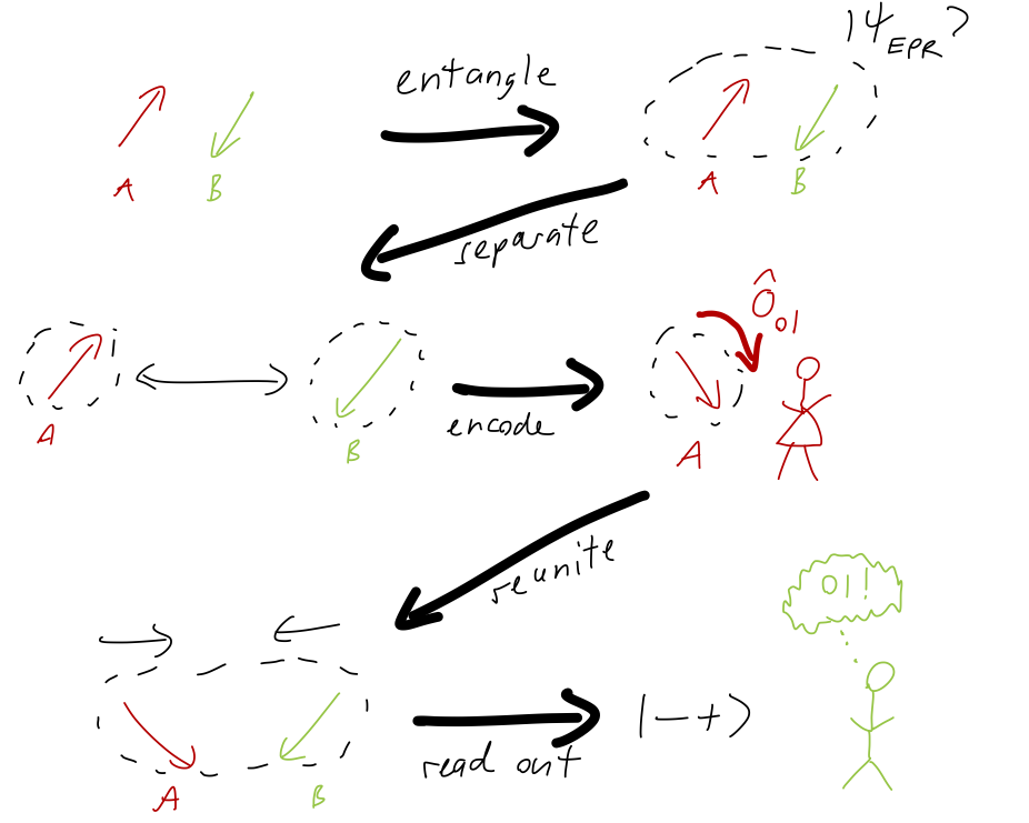
This was a lot of extra work to still send a message of only two bits, but notice what has happened: in this scheme, Alice shares an entangled qubit with Bob first, and then later only has to send one qubit to encode two bits of information. The message is entirely contained in the second qubit, in the sense that there is no information in the initial EPR pair. In a sense, all of the information is in the second qubit and in the entanglement with the first qubit.
In addition to the density of information sent per bit being twice as high, there is another interesting effect of the superdense coding protocol. If an eavesdropper (by convention always called Eve) intercepts the qubit that Alice has sent to Bob, it is useless - there is no possible measurement on qubit B alone that will allow Eve to definitely reveal what operation Alice did. Only with both entangled qubits together can the information be accessed and decoded. Even better, if Eve tries to take a measurement, the state will be altered and Alice and Bob can find out later that someone tried to intercept the message. Quantum communications can be very secure indeed!
In the superdense coding protocol, we transfer information from two classical bits into the construction of a particular quantum state. This is used for secure and dense communication, but when framed in this way, another obvious use case would be sharing classical information in order to share a copy of a quantum state.
Unfortunately, quantum correlations are subtle and delicate; it turns out to be impossible to make a perfect copy of an arbitrary quantum state. However, we can use a rearrangement of the superdense coding protocol to perform something called quantum teleportation, a name which tends to make people think of Star Trek but embodies a much simpler statement: we can send a copy of a quantum state using classical information, but only at the cost of measurements which destroy the original state.
15.4.2 No-cloning theorem
Before we get to teleportation, let’s be more rigorous about the statement that “it’s impossible to make a perfect copy of a quantum state” - a result known as the no-cloning theorem.
To explain the no-cloning theorem, we will return to our quantum communication example and see what our eavesdropper Eve is capable of doing. She knows that a measurement of the qubit B which is being sent will change the state and reveal her presence. But what if she could simply make a copy of the qubit, and then measure that instead? She uses a third qubit E, and she wants to apply a quantum process that will take it from some arbitrary initial state into a copy of B: \hat{U}_{\rm copy} (\ket{\psi}_B \otimes \ket{\uparrow}_E) = \ket{\psi}_B \otimes \ket{\psi}_E. I’ve written \hat{U}_{\rm copy} to indicate this should be a unitary operation: whatever the physical process is that allows Eve to make a copy, it is described by some quantum Hamiltonian \hat{H}_{\rm copy} and she applies it for some amount of time to allow the total system to evolve. This is the only way to change a quantum system other than measurement - and measurement of \ket{\psi}_B will invariably disturb the state, which is what we are trying to avoid.
The problem is that no such unitary operation can exist! To see why, suppose that Eve uses the same operation to copy a second state \ket{\phi}_B. Before the copying operation is applied, the inner product between the two states is c_0 = \left\langle \phi | \psi \right\rangle. But after applying \hat{U}_{\rm copy}, if we take the inner product again we get c_1 = \left\langle \phi | \psi \right\rangle^2. This means that the copying operation can’t be unitary, since unitary operations preserve inner products!
There are a couple of ways we can generalize this argument to make it into a full “proof”; I won’t be exhaustive here, but let’s consider one possible improvement, which is that Eve’s Hilbert space \mathcal{H}_E is arbitrary and can be much larger than the space \mathcal{H}_B of the state she’s trying to duplicate. This means that we allow the copying process to produce a different state: \hat{U}_{\rm copy}' (\ket{\psi}_B \otimes \ket{\uparrow}_E) = \ket{\psi}_B \otimes \ket{\Psi}_E. Ideally, \ket{\Psi}_E is a much larger state that we can apply some measurements to in order to reconstruct information about \ket{\psi}_B. But now, let’s again suppose she tries to copy two different states: \ket{C_1} = \hat{U}_{\rm copy}' (\ket{\psi}_B \otimes \ket{\uparrow}_E) = \ket{\psi}_B \otimes \ket{\Psi}_E, \\ \ket{C_2} = \hat{U}_{\rm copy}' (\ket{\phi}_B \otimes \ket{\uparrow}_E) = \ket{\phi}_B \otimes \ket{\Phi}_E. Once again since the evolution is unitary, the inner product must be preserved. In this case, we have before the copy \left\langle C_1 | C_2 \right\rangle = {}_B\! \left\langle \phi | \psi \right\rangle_B since {}_E\! \left\langle \uparrow | \uparrow \right\rangle_E = 1. Then after copying, \left\langle C_1 | C_2 \right\rangle = {}_B\! \left\langle \phi | \psi \right\rangle_B {}_E\! \left\langle \Phi | \Psi \right\rangle_E. These have to be equal, which means that {}_E\! \left\langle \Phi | \Psi \right\rangle_E = 1. But this means that \ket{\Phi}_E and \ket{\Psi}_E are the same state, even if (as we have assumed) \ket{\psi}_B and \ket{\phi}_B are different! This setup demonstrates that not only are we unable to copy the original states with a unitary process, we can’t obtain any information at all about the state of B with a unitary process like this. The only thing Eve can do is measure - which in the superdense coding example would give her some information, but not enough to get the whole message, and would also alert Alice and Bob to her eavesdropping.
The no-cloning theorem is not very surprising given what we know about quantum mechanics. With the way that measurement works in quantum systems, it’s impossible to completely characterize a given quantum state \ket{\psi}, since we can’t know the results of all possible measurements. Of course, the simplest way to end-run around the no-cloning theorem is to simply have a process that creates a known quantum state. Then with an ensemble of identical states, we can take all the measurements we want to try to reconstruct what state our process is producing. This practice of reconstructing a quantum state from measurement of an identical collection of such states is known as quantum tomography.
15.4.3 Quantum teleportation
Now let’s come back to the detailed construction of how Alice can send an arbitrary quantum state \ket{\psi} to Bob, using essentially a variation of the superdense coding protocol. This process, known as quantum teleportation, was proposed in 1993 and realized experimentally a few years later by Popescu and Zeilinger.
This time the process involves three qubits, with one qubit O storing the original quantum state, and then an entangled EPR pair A and B again. The arbitrary state can be written as \ket{\psi}_O = c_+ \ket{\uparrow}_O + c_- \ket{\downarrow}_O. Let’s consider the joint quantum state \ket{\Psi} of all three qubits. The A and B qubits are constructed in an EPR state as before, while O is left separate. Since O isn’t entangled, the joint state is a simple direct-product state: \ket{\Psi} = \ket{\psi}_O \otimes \ket{\psi_{EPR}}_{AB} \\ = \frac{1}{\sqrt{2}} \left( c_+ \ket{\uparrow}_O \ket{\uparrow}_A \ket{\downarrow}_B - c_+ \ket{\uparrow}_O \ket{\downarrow}_A \ket{\uparrow}_B + c_- \ket{\downarrow}_O \ket{\uparrow}_A \ket{\downarrow}_B - c_- \ket{\downarrow}_O \ket{\downarrow}_A \ket{\uparrow}_B \right). Next, we can recognize that the four different combinations of spins O and A appearing in the total state can be rewritten in terms of the \{\hat{O}_1, \hat{O}_2\} CSCO that we used above. The basis rotation is \ket{\uparrow} \ket{\uparrow} = -\frac{1}{\sqrt{2}} (\ket{\psi_x} + i \ket{\psi_y}) \\ \ket{\uparrow} \ket{\downarrow} = \frac{1}{\sqrt{2}} (\ket{\psi_{EPR}} + \ket{\psi_z}) \\ \ket{\downarrow} \ket{\uparrow} = \frac{1}{\sqrt{2}} (\ket{\psi_{EPR}} - \ket{\psi_z}) \\ \ket{\downarrow} \ket{\downarrow} = \frac{1}{\sqrt{2}} (\ket{\psi_x} - i\ket{\psi_y}). So the total state \ket{\Psi} can also be written as \ket{\Psi} = \frac{1}{2} \left[ \ket{\psi_{EPR}}_{OA} (-c_+ \ket{\uparrow}_B + c_- \ket{\downarrow}_B)) - \ket{\psi_x}_{OA} (-c_- \ket{\uparrow}_B -c_+ \ket{\downarrow}_B) \right. \\ \left. +i \ket{\psi_y}_{OA} (c_- \ket{\uparrow}_B - c_+ \ket{\downarrow}_B ) - \ket{\psi_z}_{OA} (c_+ \ket{\uparrow}_B + c_- \ket{\downarrow}_B) \right]. We now have four basis states in the CSCO for the combination of Alice’s two spins, each multiplied by another state for Bob’s spin which encodes the coefficients c_\pm from the original state \ket{\psi}_O. This gives us a simple protocol for “teleportation” (copying the original state):
As with superdense coding, Alice and Bob create an entangled pair in an EPR state and then each take one of the qubits.
Alice measures with the pair of operators \hat{O}_1 = \hat{S}_{x,O} \otimes \hat{S}_{x,A} and \hat{O}_2 = \hat{S}_{z,O} \otimes \hat{S}_{z,A}, and records the measurement outcomes. This collapses the two qubits O and A into one of the four entangled CSCO basis states we wrote out above.
Alice tells Bob the results of her two measurements, o_1 = \pm 1 and o_2 = \pm 1. This tells Bob exactly which of the four states his qubit is in.
Finally, Bob applies a unitary operation to rotate the state he has into the original state \ket{\psi}. For example, if Alice’s measurements inform her that her state has collapsed to \ket{\psi_z}_{OA}, then Bob already has \ket{\psi} up to a minus sign. If she finds \ket{\psi_x}, then Bob just needs to apply \hat{\sigma}_{x,B} to swap the spin states to recover \ket{\psi}, and so on.
Once more, here is a sketch overview, showing many of the similarities between quantum teleportation and superdense coding:
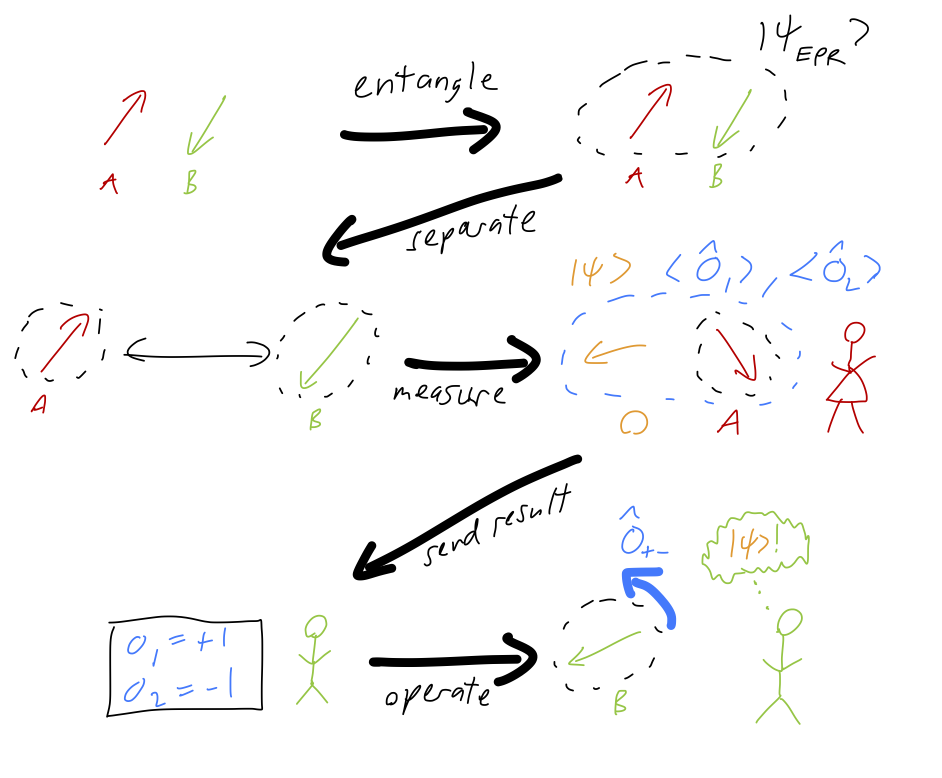
The outcome of all of this is that the original state \ket{\psi}_O has been transferred completely onto the qubit B that Bob has, without disturbing it (or revealing any information about c_\pm.) The reason this is called “teleportation” is that this process of copying the state can be done over arbitrarily long distances, once the initial entangled EPR pair has been shared. But like the EPR and Bell example considered above, there is still nothing non-local happening; the transfer of the state still requires the classical information about the outcomes of Alice’s measurements to be sent to Bob, which can’t be done any faster than the speed of light. Once again, we’re just seeing a counterintuitive effect that relies on the nature of quantum correlations.