5 Position and momentum operators
Now that we have some experience with finite-dimensional Hilbert spaces, we’re ready to see how this formalism lets us connect back to the language of wavefunctions that you are probably familiar with. We’ll find that the wavefunction emerges naturally when we try to consider position as an operator. Position has a continuous spectrum, but by the postulates the outcome of a position measurement must be an eigenvalue; to reconcile these two points, we need an infinite-dimensional Hilbert space (since there are an infinite number of positions we can measure.)
By design, the mathematics of continuous observables doesn’t look very different! If \hat{\xi} is an observable in an infinite-dimensional space, then its eigenvalue equation looks familiar: \hat{\xi} \ket{\xi} = \xi \ket{\xi} There are some small differences when we go from discrete to continuous:
- Sums should be replaced with integrals, e.g. in the completeness relation
\hat{1} = \int d\xi\ \ket{\xi}\bra{\xi}
- Kronecker delta functions should be replaced with Dirac delta functions, e.g. in the orthogonality relation
\left\langle \xi | \xi' \right\rangle = \delta(\xi - \xi')
- We can no longer use finite matrices and vectors to represent operators and states. We can still expand an arbitrary state vector in a continuous basis, \ket{\psi} = \int d\xi\ \ket{\xi} \left\langle \xi | \psi \right\rangle. but now the infinite set of coefficients \left\langle \xi | \psi \right\rangle is a single continuous function instead of a vector: \left\langle \xi | \psi \right\rangle \rightarrow \psi(\xi).
The Dirac delta function is defined to be zero at every point, except where its argument is zero. Although it is only non-zero for an infinitesmal span, the area under the delta function is constant: \int dx\ \delta(x) = 1. If we integrate another function times the delta function, we “pick out” the one point where the argument of \delta(x) is zero: \int dx\ \delta(x-a) f(x) = f(a). The delta function “collapses” the integral, selecting out a single value of the function; this is similar to what the Kronecker delta does to sums. Note that I haven’t included limits of integration; these identities are true when we integrate over any integral that contains the non-zero part of \delta(x).
As I mentioned, strictly speaking \delta(x) is not a function; you should be very careful with its interpretation when it’s not safely under an integral! When in doubt, you can fall back on a more rigorous definition in terms of a limit of a set of functions; there’s more than one definition, but one useful construction is a Gaussian distribution with vanishing width: \delta(x) = \lim_{a \to 0} \frac{1}{\sqrt{\pi} a} \exp \left( - \frac{x^2}{a^2} \right).
You can verify that this definition recovers the integral properties we found above. We can also use it to derive some more useful properties: \delta(-x) = \delta(x) \\ \delta'(-x) = -\delta'(x) \\ x \delta'(x) = -\delta(x) \\ \delta (ax) = \frac{1}{|a|} \delta(x) \\ \delta(x^2 - a^2) = \frac{1}{2|a|} [ \delta(x+a) + \delta(x-a) ] More generally, for any function inside the \delta we have \delta(f(x)) = \sum_i \frac{\delta(x-x_i)}{|f'(x_i)|} where x_i are the roots of f(x), i.e. f(x_i) = 0. (If you want to see why this last property is true, use the limit representation and Taylor expand about the roots.)
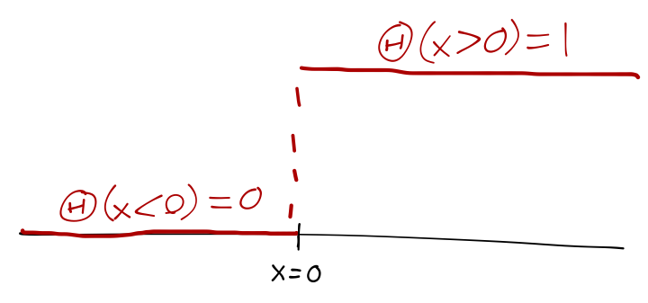
A related special function is obtained if we integrate the Dirac delta from -\infty to x, which gives either 0 or 1, depending on whether our integration includes x=0. This defines the Heaviside step function \Theta(x), \Theta(x) \equiv \int_{-\infty}^x dx'\ \delta(x') = \begin{cases} 0, & x<0; \\ 1, & x\geq 0 \end{cases}.
Here’s a summary table comparing some important expressions in discrete vs. continuous notation:
| Discrete | Continuous | |
|---|---|---|
| Completeness | \hat{1} = \sum_a \ket{a} \bra{a} | \hat{1} = \int d\xi\ \ket{\xi} \bra{\xi} |
| Orthogonality | \left\langle a_i | a_j \right\rangle = \delta_{ij} | \left\langle \xi | \xi' \right\rangle = \delta(\xi-\xi') |
| Expansion in basis | \ket{\psi} = \sum_i \ket{a_i} \left\langle a_i | \psi \right\rangle = \sum_i c_i \ket{a_i} | \ket{\psi} = \int d\xi \ket{\xi} \left\langle \xi | \psi \right\rangle = \int d\xi\ \psi(\xi) \ket{\xi} |
| Normalization | \sum_i |\left\langle a_i | \psi \right\rangle|^2 = 1 | \int d\xi\ |\left\langle \xi | \psi \right\rangle|^2 = 1 |
| Matrix elements | \bra{a_i}\hat{A}\ket{a_j} = a_j \delta_{ij} | \bra{\xi}\hat{\xi}\ket{\xi'} = \xi' \delta(\xi-\xi') |
You can see that we’re getting close to recovering the wavefunction of wave mechanics! Let’s add the last missing piece by considering our first concrete example of a continuous operator: the position operator.
5.1 The position operator
Let’s consider our first concrete example of a continuous operator; the position operator. This will take us back to the familiar wavefunction. We’ll begin by sticking to one dimension, so the position operator \hat{x} corresponding to the position of a particle has no vector index.
Position is continuous, so we have an infinite basis given by \hat{x} \ket{x} = x \ket{x} leading to the matrix elements \bra{x'} \hat{x} \ket{x} = x \delta(x'-x) and an arbitrary state can be written as \ket{\psi} = \int_{-\infty}^\infty dx\ \ket{x}\left\langle x | \psi \right\rangle = \int_{-\infty}^\infty dx\ \psi(x) \ket{x}. Just like any other observable, position satisfies the “collapse” postulate; if we measure the position of a particle and find it to be x, then the state vector collapses from \ket{\psi} \rightarrow \ket{x}. This isn’t fully realistic, since real position measurements don’t have infinite precision, but it’s a reasonable approximation for most purposes.
What is the probability of measuring a range of positions? We haven’t thought much about “ranges” of outcomes before, since this is our first encounter with a continuous observable. We know that the probability of finding a particular value of x as the outcome is, from Born’s rule, p(x) = |\left\langle x | \psi \right\rangle|^2 = |\psi(x)|^2. But since there are an infinite number of possible x outcomes, if we properly normalize our state this number is infinitesimal, basically equal to zero. That doesn’t mean it’s unphysical; it simply means that we must interpret |\psi(x)|^2 as a probability density function (pdf), which is the familiar statement from undergrad quantum for the wavefunction \psi(x). As usual for a pdf, probabilities of single outcomes are not really meaningful, but we can integrate to get probabilities of ranges of outcomes:
p(x \in [x_1, x_2]) = \int_{x_1}^{x_2} dx\ |\psi(x)|^2.
This is the more realistic thing to deal with in practice, since real experiments always have some measurement uncertainty; we’ll never really measure an exact value of the position x.
You might be concerned that there is something less than rigorous hiding in the derivation above; I’m arguing that |\psi(x)|^2 is a pdf, but I’m also admitting that the individual probabilities it computes are basically zero and not meaningful unless integrated. Is it really a pdf, and is my formula for measurement outcome in a range correct? Here is an alternative approach that starts with the idea of a more realistic measurement and goes from there, no hand-waving required.
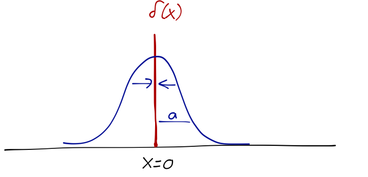
Assume that we have some measurement error \Delta, so that the best we can do is pinpoint the position to be within the interval [x-\Delta, x+\Delta]. Then the collapse of the state after such a measurement will be a projection onto the set of \hat{x} eigenstates within this spatial interval.
We can construct an operator associated with this projection as an outer product, like this: \hat{M}(x, \Delta) = \int_{x-\Delta}^{x+\Delta} dx'\ \ket{x'} \bra{x'} = \int_{-\infty}^\infty dx'\ \ket{x'} \bra{x'} (\Theta(x'-x+\Delta) - \Theta(x'-x-\Delta)) where I’ve used the difference of step functions to construct a “boxcar function” that selects the chosen interval. Its matrix element between two position eigenstates is \bra{x'} \hat{M}(x, \Delta) \ket{x''} = \int_{-\infty}^\infty dx'''\ \left\langle x' | x''' \right\rangle \left\langle x''' | x'' \right\rangle \left( \Theta(x'''-x+\Delta) - \Theta(x'''-x-\Delta) \right) \\ = \delta(x'-x'') \left( \Theta(x'-x+\Delta) - \Theta(x'-x-\Delta) \right). This means that for an arbitrary physical state, the expectation value of our measurement is \bra{\psi} \hat{M}(x, \Delta) \ket{\psi} = \int dx' \int dx''\ \left\langle \psi | x' \right\rangle \bra{x'} \hat{M} \ket{x''} \left\langle x'' | \psi \right\rangle \\ = \int dx' \int dx''\ \left\langle \psi | x' \right\rangle \delta(x'-x'') \left( \Theta(x'-x+\Delta) - \Theta(x'-x-\Delta) \right) \left\langle x'' | \psi \right\rangle \\ = \int_{x-\Delta}^{x+\Delta} dx'\ |\left\langle \psi | x' \right\rangle|^2 = \int_{x-\Delta}^{x+\Delta} dx' |\psi(x')|^2. How do we interpret this expectation value? Measuring a projection like this simply tells us if our particle exists in the region [x-\Delta, x+\Delta] or not; the value of \left\langle \hat{M} \right\rangle will vary from zero (if \psi(x) = 0 everywhere in the region, i.e. we never find our particle here) to one (if \psi(x) = 0 everywhere outside the region.) Thus, \left\langle \hat{M}(x,\Delta) \right\rangle is precisely the probability to find our particle in [x-\Delta, x+\Delta].
This shows, without bumping into any infinities or infinitesimals, that we can indeed interpret |\psi(x)|^2 as a probability density function for the x position of our particle.
As a pdf, p(x) should be normalized so that its integral over all x values is 1 (the probability of finding our particle anywhere at all should be 1): \left\langle \psi | \psi \right\rangle = \int_{-\infty}^\infty dx\ |\psi(x)|^2 = 1. This is equivalent to the statement that the norm of the state \left\langle \psi | \psi \right\rangle = 1. More generally, the inner product of two states is now also given by an integral, \left\langle \phi | \psi \right\rangle = \int_{-\infty}^\infty dx\ \left\langle \phi | x \right\rangle \left\langle x | \psi \right\rangle = \int_{-\infty}^\infty dx\ \phi^\star(x) \psi(x). and matrix elements between arbitrary states by a double integral: \bra{\phi} \hat{A} \ket{\psi} = \int dx \int dx'\ \left\langle \phi | x \right\rangle \bra{x} \hat{A} \ket{x'} \left\langle x' | \psi \right\rangle \\ = \int dx \int dx'\ \phi^\star(x) \bra{x} \hat{A} \ket{x'} \psi(x). If \hat{A} = {A}(\hat{x}) is purely a function of the position operator \hat{x}, then its matrix elements are A(x) \delta(x-x'), and the integral collapses, giving us \left\langle A(\hat{x}) \right\rangle = \int_{-\infty}^\infty dx\ A(x) |\psi(x)|^2. This is the usual definition of an expectation value over the probability density |\psi(x)|^2. But keep in mind that the fundamental quantity here is \psi, not its square!
The fact that quantum mechanical states are described by probability amplitudes (which square to give probabilities) is a source of much of the interesting quantum behavior we will see. In classical probability theory, if we have two events A and B which are independent (e.g. rolling 1 and 5 on two different dice at once), then the probability of joint event A \cap B is given by the product p(A \cap B) = p(A) p(B). On the other hand, if A and B are mutually exclusive (rolling 1 or 5 on the same die at once), then the probability of measuring either event A or event B is given by the sum, p_{\rm classical}(A \cup B) = p(A) + p(B). In quantum mechanics, the first rule still holds. However, the big difference in a quantum world is that for exclusive outcomes (like, say, an electron passing through one of two openings in a screen), it’s not the probabilities but the amplitudes which add: \psi(A \cup B) = \psi(A) + \psi(B), so that p_{\textrm{quantum}}(A \cup B) = |\psi(A) + \psi(B)|^2 = p(A) + p(B) + 2 \textrm{Re}(\psi^\star(A) \psi(B)). This extra interference term between exclusive events is at the core of quantum behavior, as we’ve seen in our specific example involving Stern-Gerlach like experiment before; but it’s worth repeating in this more general and simplified way.
5.2 The momentum operator
As we have just showed, if an observable \hat{A} is just some function of position, then the matrix elements with the position eigenkets are simple: \bra{x} \hat{A} \ket{x'} = A(x') \delta(x-x') and the general matrix element collapses to a single integral. But not every operator is just a function of position! For example, we can introduce a momentum operator \hat{p}, which measures the momentum of our particle (still in one dimension.)
How do we calculate \bra{x} \hat{p} \ket{x'}? It should be obvious that momentum eigenstates cannot also be position eigenstates; momentum implies movement, which is a change of position. Sakurai gives a long discussion of the relation between momentum and change in position (aka translation) in section 1.6; I want to defer that study until we get to a more detailed treatment of symmetries in quantum mechanics, so don’t worry if you didn’t follow that section right now. Instead I am going to start with the canonical commutation relation,
The position operator \hat{x} and the momentum operator \hat{p} obey the canonical commutation relation [\hat{x}, \hat{p}] = i\hbar.
Some books treat this as another postulate; you can also think of it as a definition of momentum and/or of Planck’s constant \hbar.
This commutator is all we need to determine what \hat{p} must look like in coordinate space. If we sandwich the commutator between an arbitrary pair of states, we have \bra{\phi} [\hat{x}, \hat{p}] \ket{\psi} = \int dx \int dx'\ \left\langle \phi | x \right\rangle \bra{x} \hat{x} \hat{p} - \hat{p} \hat{x} \ket{x'} \left\langle x' | \psi \right\rangle \\ = \int dx \int dx'\ \phi^\star(x) (x \bra{x}\hat{p}\ket{x'} - \bra{x}\hat{p}\ket{x'} x') \psi(x') where we can act either to the left or to the right with \hat{x}, since it’s an observable and therefore Hermitian. By the canonical commutation relation, this must be equal to \bra{\phi} [\hat{x}, \hat{p}] \ket{\psi} = i \hbar \left\langle \phi | \psi \right\rangle = i\hbar \int dx\ \phi^\star(x) \psi(x). No function of \hat{x} can satisfy this relation; basically, the matrix element we want should contain something like a Dirac delta \delta(x-x') to collapse two integrals down to one - but then the two terms in the first expression above will immediately give zero when x = x'! If you stare at the expressions long enough, you can verify that the solution to this equation must involve a derivative as the matrix element: \bra{x} \hat{p} \ket{x'} = \delta(x-x') \frac{\hbar}{i} \frac{\partial}{\partial x} In other words, we can write the wavefunction corresponding to \hat{p} acting on an arbitrary state as \bra{x} \hat{p} \ket{\psi} = \int dx'\ \bra{x} \hat{p} \ket{x'} \left\langle x' | \psi \right\rangle \\ = \int dx' \delta(x-x') \frac{\hbar}{i} \frac{\partial}{\partial x} \left\langle x' | \psi \right\rangle \\ = \frac{\hbar}{i} \frac{\partial \psi(x)}{\partial x}. Clearly, acting with momentum repeatedly just gives more derivatives, so matrix elements for powers of \hat{p} can be written as: \bra{\phi} \hat{p}{}^n \ket{\psi} = \int dx\ \phi^\star(x) \left( \frac{\hbar}{i} \frac{\partial}{\partial x} \right)^n \psi(x). The canonical commutation relation tells us, unsurprisingly, that \hat{x} and \hat{p} are incompatible observables; they have no simultaneous eigenstates. Applying the uncertainty relation gives us the familiar Heisenberg uncertainty principle for position and momentum, \Delta x \Delta p \geq \hbar/2. Of course, the momentum operator has its own orthonormal basis of state with definite momentum, \hat{p} \ket{p} = p \ket{p}. Given a particular physical state, we can expand it instead in momentum eigenstates: \ket{\psi} = \int dp\ \ket{p} \left\langle p | \psi \right\rangle = \int dp\ \ket{p} \tilde{\psi}(p) where now \tilde{\psi}(p) is the momentum-space wavefunction, denoted in my notation with a tilde. (Sometimes you’ll see people use \phi for a generic momentum-space wavefunction complementary to \psi; I prefer the tilde since it’s more general.)
5.3 Relation between the bases
Just as in the finite-dimensional case, we can compute a change of basis from position to momentum space, or vice-versa: \left\langle x | \psi \right\rangle = \int dp\ \left\langle x | p \right\rangle \left\langle p | \psi \right\rangle The overlap between the two basis states isn’t immediately obvious, but we can figure it out. Since we’re integrating over p we want to find the function \left\langle x | p \right\rangle in momentum space. Notice that \bra{x} \hat{p} \ket{p} = p \left\langle x | p \right\rangle = \frac{\hbar}{i} \frac{\partial}{\partial x} \left\langle x | p \right\rangle. This is just a differential equation, which you should recognize the solution to right away: \left\langle x | p \right\rangle = \frac{1}{\sqrt{2\pi \hbar}} \exp \left( \frac{ipx}{\hbar} \right) (where the normalization ensures that \left\langle x | x' \right\rangle = \delta(x-x') when we insert a complete set of \ket{p} states.)
Although we’re about to use this to change bases, I’ll stop and point out that this also tells us what a momentum eigenstate looks like in position space: an oscillating, complex exponential which is periodic under x \rightarrow x + 2\pi \hbar / p \equiv x + 2\pi/k. This is called a plane wave, and the quantity k with units of inverse length is the wave number. As we would expect, the plane wave is a state which is absolutely localized in momentum space at p, and is therefore completely delocalized in position space: if we calculate the mean and variance (regulating things carefully to avoid ambiguity), we will find that \left\langle \hat{x} \right\rangle \rightarrow 0 but \Delta x \rightarrow \infty.
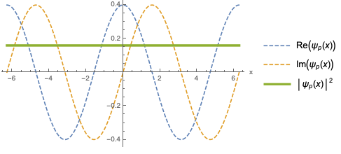
Note that this is one of the examples I mentioned where you need to be cautious with delta functions and infinities! If you try to make sure the plane wave solution is normalized, you will find that \int_{-\infty}^\infty dx\ |\left\langle x | p \right\rangle|^2 = \int_{-\infty}^\infty dx\ \frac{1}{2\pi \hbar} \exp \left(\frac{ipx}{\hbar} - \frac{ipx}{\hbar} \right) = \infty which looks like a disaster! In fact, we can write this a bit more generally noticing that if we tried to integrate over two different momentum eigenstates, then the result is zero. (You can do this by rewriting the integral as a contour integral in the complex plane, noticing that there are no poles inside the residue, and that as long as p \neq p' the integral off the real line will be exponentially damped.) In fact, we know from our definitions in Hilbert space that we must have \left\langle p | p' \right\rangle = \delta(p-p'). We accept such improperly normalized states into our Hilbert space, because they are useful to think about in certain situations. In practice, any physical system will be localized to some finite region of space and we won’t have to worry about this subtle divergence.
We can carry through a similar argument to go in the opposite direction, i.e. to find the position eigenstates in momentum space. It won’t surprise you that the operator \hat{x} acts as a derivative in momentum space, except with the i upstairs: \bra{p} \hat{x} \ket{p'} = \delta(p-p') i\hbar \frac{\partial}{\partial p}. In fact, in momentum space we find exactly the same function for the product \left\langle x | p \right\rangle. What we’ve proved is that the functions representing a particular state in position and momentum space are nothing but Fourier transforms of one another: \psi(x) = \frac{1}{\sqrt{2\pi \hbar}} \int dp\ \exp \left(\frac{ipx}{\hbar} \right) \tilde{\psi}(p) \\ \tilde{\psi}(p) = \frac{1}{\sqrt{2\pi \hbar}} \int dx\ \exp \left(\frac{-ipx}{\hbar} \right) \psi(x).
5.4 Wave packets
The step-function example of a localized position state that we constructed above as a projection operator wasn’t very realistic. A more practical construction is an object known as the Gaussian wave packet. We define such a state through its position space wave function, \left\langle x | \psi \right\rangle = \psi(x) = \frac{1}{\pi^{1/4} \sqrt{d}} \exp \left( ikx - \frac{x^2}{2d^2} \right). To construct this state we’ve started with a plane wave of wave number k, and then modulated it with (multiplied by) a Gaussian distribution centered at x=0 with width d. The Gaussian envelope localizes our state near x=0; the real and imaginary parts of the amplitude in x (arbitrarily taking d=1) now look like this:
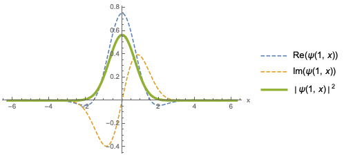
where I’ve overlaid the probability density |\psi(x)|^2, which is Gaussian. Clearly this looks localized, but let’s actually go through the exercise of calculating the expectation values for position. The mean is given by \left\langle \hat{x} \right\rangle = \int_{-\infty}^\infty dx \left\langle \psi | x \right\rangle x \left\langle x | \psi \right\rangle = \int_{-\infty}^\infty dx\ |\psi(x)|^2 \\ = \frac{1}{\sqrt{\pi} d} \int_{-\infty}^\infty dx\ x \exp(-x^2/d^2) = 0 since the integral is odd. For \hat{x}{}^2, things are a little tougher: \left\langle \hat{x}{}^2 \right\rangle = \frac{1}{\sqrt{\pi}d} \int_{-\infty}^\infty dx\ x^2 \exp(-x^2/d^2)
Gaussian integrals such as this one crop up everywhere in physics, so if you’re not familiar, let’s take a slight detour to study them. We start with the most basic Gaussian integral, I(\alpha) \equiv \frac{1}{\sqrt{\pi} d} \int_{-\infty}^\infty dx\ \exp(-\alpha x^2) = \sqrt{\frac{\pi}{\alpha}}. The result for \alpha = 1 was originally found by Laplace, and can be elegantly derived by squaring the integral and changing to polar coordinates. This is all we need to derive the result we need above: if we take the derivative of the integral with respect to \alpha, we find \frac{\partial}{\partial \alpha} \int_{-\infty}^\infty dx\ e^{-\alpha x^2} = -\int_{-\infty}^\infty dx\ x^2 e^{-\alpha x^2}. So \int_{-\infty}^\infty dx\ x^2 e^{-\alpha x^2} = -\frac{\partial I}{\partial \alpha} = \frac{\sqrt{\pi}}{2\alpha^{3/2}}. For higher even powers of x, we just take more derivatives with respect to \alpha; all the odd powers vanish. The general result for n even can be shown to be \int_{-\infty}^\infty dx\ x^n e^{-\alpha x^2} = \frac{(n-1)!! \sqrt{\pi}}{2^{n/2} \alpha^{(n+1)/2}}. where !! is the double factorial symbol, (n+1)!! = (n+1)(n-1)...(5)(3)(1).
I’ll finish this example in one dimension, but as long as we’re doing math, I’ll remark on the generalization to multi-dimensional Gaussian integrals. With n coordinates, the most general pure Gaussian integral we can write is \int d^n x \exp \left( -\frac{1}{2} \sum_{i,j} A_{ij} x_i x_j \right) = \int d^n x \exp \left( -\frac{1}{2} \vec{x}^T \mathbf{A} \vec{x} \right) = \sqrt{\frac{(2\pi)^n}{\det \mathbf{A}}}, where the 1/2 is conventional, and the result is most nicely expressed by thinking of the various numbers A_{ij} as forming a matrix \mathbf{A}. Using derivatives with respect to A_{ij} on this expression can similarly give us more complicated functions to integrate against, just with more algebra than the 1-d case.
Back to our wave packet: the dispersion in \hat{x} is now seen to be \left\langle \hat{x}{}^2 \right\rangle = \frac{1}{\sqrt{\pi} d} \frac{\sqrt{\pi}d^3}{2} = \frac{d^2}{2}. so \Delta x = \sqrt{\left\langle \hat{x}{}^2 \right\rangle - \left\langle \hat{x} \right\rangle^2} = d/\sqrt{2}.
What about the momentum? We started with a plane wave of definite momentum \hbar k, but the convolution with the Gaussian will have changed that. Being careful about the order now, we can see that the expectation value of \hat{p} is \left\langle \hat{p} \right\rangle = \int_{-\infty}^\infty dx\ \int_{-\infty}^\infty dx'\ \left\langle \psi | x \right\rangle \bra{x} \hat{p} \ket{x'} \left\langle x' | \psi \right\rangle\\ = \int_{-\infty}^\infty dx\ \int_{-\infty}^\infty dx'\ \psi^\star(x) \left( -i\hbar \delta(x-x') \frac{\partial}{\partial x} \right) \psi(x') \\ = \frac{-i\hbar}{\sqrt{\pi} d} \int_{-\infty}^\infty dx\ e^{-ikx - x^2/(2d^2)} \left(ik - \frac{x}{d^2} \right) e^{ikx-x^2/(2d^2)} \\ = \frac{\hbar k}{\sqrt{\pi d}} (\sqrt{\pi} d) = \hbar k where the second term proportional to x/d^2 is odd in x and vanishes identically. So the Gaussian convolution didn’t change the mean value of the momentum from the plane wave we started with. However, there is now some dispersion in the momentum; you can verify that \left\langle \hat{p}{}^2 \right\rangle = \frac{\hbar^2}{2d^2} + \hbar^2 k^2, which gives \Delta p = \frac{\hbar}{\sqrt{2} d}. Notice that if we try to explicitly check the uncertainty relation, we find that \Delta x \Delta p \geq \frac{1}{2} \left|\left\langle [\hat{x}, \hat{p}] \right\rangle\right| \\ \Rightarrow \hbar/2 \geq \hbar/2. Not only does our wave packet satisfy the uncertainty relation, it saturates it; we have an equality. The Gaussian wave packet is known as the minimum uncertainty wave packet because it gives the smallest product of uncertainties \Delta x \Delta p.
What does the wave packet look like in terms of momentum? We can easily carry out the Fourier transform: \tilde{\psi}(p) = \int dx \left\langle p | x \right\rangle \left\langle x | \psi \right\rangle \\ = \frac{1}{\sqrt{2\pi \hbar}} \int dx\ \exp\left(\frac{-ipx}{\hbar}\right) \frac{1}{\pi^{1/4} \sqrt{d}} \exp \left(ikx - \frac{x^2}{2d^2} \right) \\ = \frac{1}{\sqrt{2\hbar d} \pi^{3/4}} \int dx\ \exp \left[ -\left(\frac{x}{\sqrt{2}d} -\frac{id(k-p/\hbar)}{\sqrt{2}}\right)^2 - \frac{d^2 (p-\hbar k)^2}{2\hbar^2}\right] completing the square. But this is an integral from -\infty to \infty, so we can just shift the integration to the squared quantity, and we have an ordinary Gaussian integral with dx' = dx/(\sqrt{2}d). Thus: \tilde{\psi}(p) = \frac{1}{\sqrt{2\hbar d} \pi^{3/4}} \exp \left(\frac{-d^2(p-\hbar k)^2}{2\hbar^2}\right) \sqrt{2}d \int_{-\infty}^\infty dx'\ e^{-x'{}^2} \\ = \frac{1}{\pi^{1/4} \sqrt{\hbar/d}} \exp \left( \frac{-(p-\hbar k)^2}{2(\hbar/d)^2} \right). This is, once again, a Gaussian distribution, this time with mean value \hbar k and variance \hbar^2/2d^2, exactly as we found from the x wavefunction directly. You can evaluate these expectation values directly, or you can just read them off of the distribution; we know that |\tilde{\psi}(p)|^2 is a Gaussian probability density, which takes the generic form we saw previously p(\mu, \sigma) = \frac{1}{\sqrt{2\pi} \sigma} e^{-(x-\mu)^2/(2\sigma^2)} for mean \mu and variance \sigma^2. Notice that, unsurprisingly, the width of the momentum Gaussian packet is proportional to 1/d, whereas in position space it goes as d. The more we squeeze the spread of momentum states, the wider the distribution in position becomes, and vice-versa; this behavior is a consequence of the uncertainty relation. In the limit d \rightarrow \infty we recover the plane wave; a delta-function in p-space and an infinite wave in x-space.
5.5 The Hamiltonian operator
Now that we have a handle on the position and momentum operators, we can construct a number of other interesting observables from them. The most important is the Hamiltonian, \hat{H}. In many classical systems, we know how to write the Hamiltonian in terms of position and momentum, which naturally maps onto the quantum version of the same system. For a single particle with mass m moving in a potential energy function V(x), a quite generic classical Hamiltonian and its quantum counterpart are H = \frac{p^2}{2m} + V(x) \Rightarrow \hat{H} = \frac{\hat{p}{}^2}{2m} + V(\hat{x}).
The idea of “quantizing”, mapping a classical Hamiltonian onto its quantum counterpart, is nice and appealing, building on our intuition from classical mechanics. However, there are some problems with this approach due to the fact that as operators, \hat{x} and \hat{p} don’t commute. As a simple example, if our Hamiltonian contains the product xp, should the corresponding quantum operator by \hat{x} \hat{p}, or \hat{p} \hat{x}? A trivial way to resolve this that will generally always give the right classical limit is to symmetrize, i.e. in the quantum theory we adopt (\hat{x} \hat{p} + \hat{p} \hat{x})/2.
However, symmetrizing doesn’t always save us! The operator x^2 p^2, for example, can be implemented as (\hat{x}^2 \hat{p}^2 + \hat{p}^2 \hat{x}^2) or as (\hat{x} \hat{p} + \hat{p} \hat{x})^2 - both symmetric, but not equal in a quantum theory, even though they have the same classical limit! Ultimately, quantum mechanics is the more fundamental theory, so there’s no reason to expect we should be able to take a classical theory and “promote” it; only one of the two symmetrizations given above is the “right” theory of nature.
For an eigenstate of energy, by definition the Hamiltonian satisfies the equation \hat{H} \ket{E} = E \ket{E}. What are the matrix elements of an arbitrary state? Well, in position space: \bra{x} \hat{H} \ket{\psi} = \int dx'\ \bra{x} \hat{H} \ket{x'} \left\langle x' | \psi \right\rangle \\ = \int dx'\ \left[ \bra{x} \frac{\hat{p}{}^2}{2m} \ket{x'} + \delta(x-x') V(x') \right] \psi(x') \\ = \int dx'\ \delta(x-x') \left[ \frac{1}{2m} \left( \frac{\hbar}{i} \frac{\partial}{\partial x}\right)^2 + V(x') \right] \psi(x') \\ = \left[ -\frac{\hbar^2}{2m} \frac{\partial^2}{\partial x^2} + V(x) \right] \psi(x). If the state \ket{\psi} is an energy eigenstate, then we also have \bra{x} \hat{H} \ket{\psi, E} = E \left\langle x | \psi_E \right\rangle, or -\frac{\hbar^2}{2m} \frac{\partial^2 \psi_E}{\partial x^2} + V(x) \psi_E(x) = E \psi_E(x), which you’ll recognize as the (time-independent) Schrödinger equation.
If we have a free particle, i.e. V(x) = 0, then the solution to this differential equation is simple: V(x) = 0 \Rightarrow \psi_E(x) = \exp \left(\pm ix \sqrt{\frac{2mE}{\hbar^2}} \right). This is just a plane wave with momentum p = \pm \sqrt{2mE}; unsurprisingly, in the absence of any potential, the energy eigenstates are the momentum eigenstates. The sign of the momentum can be positive or negative, which we can think of as our particle moving towards positive or negative x. In fact, it’s easy enough for us to restore the time evolution: since these are energy eigenstates, the full time-dependent solution comes from inserting the phase e^{-i\hat{H} t/\hbar} = e^{-iEt/\hbar}, giving: \psi_E(x,t) = C_+ \exp \left( ikx - iEt/\hbar \right) + C_- \exp \left( -ikx - iEt/\hbar \right), with k \equiv p/\hbar = \sqrt{2mE}/\hbar. So the C_+ plane wave is a “right-moving” solution, since the phase is unchanged after time t if x = +(E/p) t; similarly, the C_- wave is a “left-moving” solution.
In fact, we could have predicted this without solving the differential equation, even; if V(x) = 0, then the Hamiltonian is a pure function of \hat{p}, and we have [\hat{H}, \hat{p}] = 0. This means that \hat{H} and \hat{p} are simultaneously diagonalizable, and we can label the energy-momentum eigenstates as \ket{E,p}. For each energy eigenstate, we have two momentum labels \pm p corresponding to the two directions the wave can move in.
One last point: the plane-wave solutions exist for any p, positive or negative, but only positive energy E \geq 0 is allowed. If we have negative energy, then k becomes imaginary, k = i\kappa with \kappa = \sqrt{-2mE}/\hbar, leading to the solution \psi_{E < 0}(x,t) = A \exp \left(-\kappa x - iEt/\hbar \right) + B \exp \left( +\kappa x - iEt/\hbar \right). With no boundary anywhere, we see that our wavefunction diverges to infinity as x \rightarrow \pm \infty. This results in what is known as a non-normalizable state; it is even more pathological than the normalization issue with plane waves, and such E < 0 states simply don’t make sense as plane waves. (As we will see soon, E < 0 for a finite region is perfectly allowed, just not as a plane wave.)