12 Wave mechanics in three dimensions
Now we’re ready to tackle the Schrödinger equation in three dimensions. To make full use of rotational symmetry and angular momentum, we will restrict our attention to spherically symmetric potentials, V(\vec{r}) = V(r). Since \hat{L}{}^2 only depends on \theta and \phi, this ensures that \hat{L}{}^2 commutes with the Hamiltonian. We also know from the commutation relations that any of the angular momentum components \hat{L}_i will commute with \hat{L}{}^2, and since they’re all also functions of angles only, they commute with \hat{H} too. However, the components don’t commute with each other, so to get a set of simultaneously diagonalizable observables, we have to pick one of them - the standard choice is \hat{L}_z. Thus, we can choose as a “complete set of commuting observables” \textrm{CSCO}: \{\hat{H}, \hat{L}{}^2, \hat{L}_z\}. (In general, finding a CSCO is very useful - I’ll say more about the idea when we get to spin.) Our eigenstates can thus be written \ket{E, l, m}, with the usual eigenvalue equations applying for the angular momentum states, \hat{L}_z \ket{E,l,m} = \hbar m \ket{E,l,m} \\ \hat{L}{}^2 \ket{E,l,m} = \hbar^2 l(l+1) \ket{E,l,m}. Our wavefunctions can thus be written as \psi_{Elm}(r,\theta,\phi). Let’s write out the time-independent Schrödinger equation satisfied by these states: -\frac{\hbar^2}{2m} \left[ \frac{1}{r^2} \frac{\partial}{\partial r} \left( r^2 \frac{\partial}{\partial r} \right) - \frac{l(l+1)}{r^2} \right] \psi_{Elm}(r,\theta,\phi) = (E - V(r)) \psi_{Elm}(r,\theta,\phi).
12.1 Solving the angular dependence; spherical harmonics
This is a separable differential equation; in fact, because we’ve used the fact that we’re looking for eigenstates of \hat{L}{}^2, it’s only a differential equation in r. This means that the complete solution to the wavefunction is separable into radial and angular components: \psi_{Elm}(r,\theta,\phi) = R_{El} (r) Y_l^m (\theta, \phi), where the radial wavefunction can’t depend on m since that eigenvalue doesn’t appear in the equation above. The angular dependence is totally separate, and will be common to all solutions for a spherically symmetric potential.
Although they don’t appear in the Schrödinger equation, the Y_l^m functions are still tightly constrained. Since they describe all of the angular dependence of the wavefunction, we can isolate them by writing \left\langle \theta, \phi | l,m \right\rangle = Y_l^m (\theta, \phi), where I’m ignoring the radial/energy labels since it doesn’t affect the angular functions at all. This lets us obtain constraints on the Y_l^m functions from the eigenvalue equations for angular momentum. First, we see that \bra{\theta,\phi} \hat{L}_z \ket{l,m} = m \hbar \left\langle \theta, \phi | l,m \right\rangle. As we found above, acting on the left with \hat{L}_z gives -i \hbar \partial / \partial \phi, so we have -i\hbar \frac{\partial}{\partial \phi} Y_l^m (\theta,\phi) = m \hbar Y_l^m (\theta,\phi). Acting with \hat{L}{}^2 similarly gives a somewhat more complicated differential equation, \left[ \frac{1}{\sin \theta} \frac{\partial}{\partial \theta} \left( \sin \theta \frac{\partial}{\partial \theta} \right) + \frac{1}{\sin^2 \theta} \frac{\partial^2}{\partial \phi^2} + l(l+1) \right] Y_l^m(\theta, \phi) = 0. Finally, the fact that the Y_l^m are eigenfunctions gives them some nice properties, in particular the orthonormality of the eigenstates leads to a completeness relation: since \left\langle l',m' | l,m \right\rangle = \delta_{l,l'} \delta_{m,m'}, inserting a complete set of states \ket{\theta, \phi} \bra{\theta, \phi} gives the identity \int_0^{2\pi} d\phi \int_{-1}^1 d(\cos \theta)\ [Y_{l'}^{m'}]^\star (\theta,\phi) Y_l^m(\theta, \phi) = \delta_{l,l'} \delta_{m,m'}. We can also form a completeness sum over l and m, by instead taking orthogonality of the \ket{\theta, \phi} states and inserting the angular momentum eigenstates: \sum_{l=0}^\infty \sum_{m=-l}^l Y_l^m (\theta', \phi') [Y_l^m]^\star (\theta, \phi) = \delta(\phi - \phi') \delta(\cos \theta - \cos \theta').
Now let’s solve for the harmonics themselves. Starting with the \hat{L}{}^2 equation alone, we notice that it is a separable differential equation once again: we may write Y_l^m (\theta,\phi) = T(\theta) P(\phi) and then obtain \frac{1}{T(\theta)}\left[ \sin \theta \frac{\partial}{\partial \theta} \left(\sin \theta \frac{\partial}{\partial \theta} \right) + l(l+1) \sin^2 \theta \right] T(\theta) = - \frac{1}{P(\phi)} \frac{\partial^2}{\partial \phi^2} P(\phi). The left-hand side is a function only of \theta, while the right-hand side depends just on \phi, so we set them both equal to a constant, m^2. The \phi equation is easy: \left[ \frac{\partial^2}{\partial \phi^2} + m^2 \right] P(\phi) = 0 \\ \Rightarrow P(\phi) = e^{\pm i m \phi}. The sign ambiguity is fixed by the other equation we’ve been ignoring, namely the \hat{L}_z eigenvalue equation above, which requires -i\hbar \partial P(\phi) / \partial \phi = m \hbar P(\phi), and so P(\phi) = e^{im \phi}. As expected, only certain quantized values of m are allowed, because the wavefunction must be single-valued, i.e. P(\phi) = P(\phi + 2\pi). This requires m to be an integer.
If we connect back to thinking about representations of the rotation group SO(3), the observation that m must be an integer (which also requires l to be an integer) is consistent with an earlier comment about representations of SO(3), which is that only odd-dimensional representations are allowed, which correspond to integer l. The half-integer representations (as will be used for spin-1/2) are not normal representations and can’t be used for orbital angular momentum.
If we didn’t take this fact as being handed down from on high by the mathematicians, we would have just found out the same thing from looking at the solution of the Schrödinger equation here - m must be an integer for spatial wavefunctions! Moreover, if we ignored this fact and attempted to use half-integer l or m, the corresponding “spherical harmonics” we would try to derive would be nonsensical.
Now let’s go back to the \theta equation. It will be helpful to let u = \cos \theta, in which case \frac{\partial}{\partial u} = -\frac{1}{\sin \theta} \frac{\partial}{\partial \theta}, leading to \left[ \frac{\partial}{\partial u} \left( (1-u^2) \frac{\partial}{\partial u} \right) + \left( l(l+1) - \frac{m^2}{1-u^2} \right) \right] T(u) = 0 \\ (1-u^2) \frac{\partial^2 T}{\partial u^2} - 2u \frac{\partial T}{\partial u} + \left[ l(l+1) - \frac{m^2}{1-u^2} \right] T(u) = 0. For the case m=0, this is the Legendre differential equation; its solutions are the Legendre polynomials P_n(u). A shorthand way to write the polynomials, which isn’t too cumbersome for at least the first few, is Rodrigues’s formula, P_n(x) = \frac{1}{2^n n!} \frac{d^n}{dx^n} \left[ (x^2 - 1)^n \right]. The first few Legendre polynomials are worth knowing: P_0(x) = 1 \\ P_1(x) = x \\ P_2(x) = \frac{1}{2} (3x^2 - 1) \\ P_3(x) = \frac{1}{2} (5x^3 - 3x)
For m \neq 0, the equation above is known as the associated Legendre differential equation; its solutions are known as associated Legendre polynomials, but they’re a bit less commonly encountered. As you should expect, for integer l solutions to this equation are only possible for |m| < l, recovering our other limit from the commutation relations. If you’re trying to look up solutions for non-zero m to do something practical, you’d be much better off trying to look for the complete spherical harmonics themselves.
We’ve so far ignored the overall normalization of the states, but that’s fixed by the integral completeness relation between the Y_l^m’s. I’ll skip those details, but the result is, for the m=0 states, Y_l^0(\theta, \phi) = \sqrt{\frac{2l+1}{4\pi}} P_l(\cos \theta).
12.1.1 Useful properties of spherical harmonics
The formula for the general spherical harmonics can actually be written in a fairly compact way, but it’s sufficiently impractical that I won’t reproduce it here; look for Sakurai (3.6.37) if you’re curious. These days, if you’re doing something serious involving the spherical harmonics, you’ll be better off with a table or a software package like Mathematica, instead of trying to derive them yourself from recursion relations. If you do use a table, you’ll likely only find the spherical harmonics for m \geq 0 tabulated; this is because you can get the negative-m harmonics through the useful identity Y_l^{-m}(\theta, \phi) = (-1)^m [Y_l^m(\theta, \phi)]^\star. It is very helpful to know at least what the first few spherical harmonics look like explicitly, so let’s write them down: Y_0^0(\theta, \phi) = \frac{1}{\sqrt{4\pi}} \\ Y_1^0(\theta, \phi) = \sqrt{\frac{3}{4\pi}} \cos \theta \\ Y_1^1(\theta, \phi) = -\sqrt{\frac{3}{8\pi}} e^{i\phi} \sin \theta \\ Y_2^0(\theta, \phi) = \frac{1}{4}\sqrt{\frac{5}{\pi}} (3 \cos^2 \theta - 1) \\ Y_2^1(\theta, \phi) = -\frac{1}{2} \sqrt{\frac{15}{2\pi}} e^{i\phi} \sin \theta \cos \theta \\ Y_2^2(\theta, \phi) = \frac{1}{4} \sqrt{\frac{15}{2\pi}} e^{2i\phi} \sin^2 \theta You can explore some plots of the various spherical harmonics in space here; the m=0 plots you’ve probably seen before, maybe in a chemistry class as the electron orbitals in an atom.
There are “spectroscopic labels” corresponding to each of the l, which are historical labels that you have likely heard before:
| l | spec. label |
|---|---|
| 0 | s |
| 1 | p |
| 2 | d |
| 3 | f |
| 4 | g |
| … | … |
Fun fact: the first four label names are short for “sharp”, “principal”, “diffuse”, and “fundamental” (I’ve also seen “fine” for the last label, but “fundamental” seems best supported by historical literature.) These aren’t particularly intuitive so they probably won’t help you remember the notation, unfortunately. After “f” the labels just go in alphabetical order, and no longer stand for anything.
Why did I even bother introducing the Legendre polynomials? Often we will consider physical systems where l is a conserved quantum number but m is not, in which case it is very helpful to sum over products of spherical harmonics. These sums obey the addition formula, \sum_{m=-l}^{l} Y_l^m(\theta_1, \phi_1) [Y_l^m]^\star(\theta_2, \phi_2) = \frac{2l+1}{4\pi} P_l(\cos \omega) where \cos \omega = \cos \theta_1 \cos \theta_2 + \sin \theta_1 \sin \theta_2 \cos(\phi_1-\phi_2) If \phi_1 = \phi_2, then we can identify \omega = \theta_1 - \theta_2. We can think of the spherical harmonics themselves as a sort of generalization of trigonometric functions to two spherical angles instead of one polar angle; this is then a generalization of a familiar trig identity. It’s also worth noting that the Legendre polynomials satisfy P_l(1) = 1 for any l, which means that the sum of spherical harmonics with the same angles is particularly simple: \sum_{m=-l}^{l} |Y_l^m(\theta, \phi)|^2 = \frac{2l+1}{4\pi}. This is a useful identity for normalizing wavefunctions which contain spherical harmonics.
As it turns out, the spherical harmonics have distinctive properties under parity. What does a parity transformation look like in three dimensions? In terms of the rectilinear coordinates, everything just flips sign at once: x \rightarrow -x, y \rightarrow -y, z \rightarrow -z. In spherical coordinates, we have instead \hat{P} \ket{r} = \ket{r} \\ \hat{P} \ket{\theta} = \ket{\pi - \theta} \\ \hat{P} \ket{\phi} = \ket{\phi + \pi}. The addition of \pi to \phi accounts for flipping the signs of x and y, while the \theta transformation gives us the angle from the downwards-pointing z-axis. Notice that this last condition can also be written \cos \theta \rightarrow - \cos \theta.
Now, remember that we can write the spherical harmonics as separate functions of \theta and \phi: Y_l^m(\theta, \phi) = P_l^m (\cos \theta) e^{im \phi}, where P_l^m are associated Legendre polynomials. It turns out that these functions contain polynomials with either only even or only odd powers of \cos \theta, times some factors of \sin \theta which are invariant. As a result, the parity transformation in \theta has a definite effect: \hat{P} P_l^m(\cos \theta) = P_l^m(-\cos \theta) = (-1)^{l-|m|} P_l^m(\cos \theta). As for the transformation of the azimuthal part, that’s much easier to see: \hat{P} e^{im\phi} = e^{im(\phi + \pi)} = (-1)^m e^{im\phi}. Putting things together, we find \hat{P} Y_l^m (\theta, \phi) = (-1)^{l-|m|} (-1)^m Y_l^m(\theta, \phi) = (-1)^l Y_l^m(\theta, \phi) where the factor of (-1)^{m-|m|} either has an exponent of 0 or -2m, both of which give 1 since m must be an integer here. Thus, spherical harmonics with l=0,2,4... are even under parity, while l=1,3,5... are odd, independent of m. This will be a very useful property when we come to consider transition matrix elements; if we are studying a system with a Hamiltonian that respects parity, then many possible transitions can be immediately ruled out.
Once again, there is a close analogy to trigonometric functions here; the trigonometric functions \sin \theta and \cos \theta are also eigenfunctions of parity, with \hat{P} \sin \theta = -\sin \theta \\ \hat{P} \cos \theta = \cos \theta.
12.2 Wave mechanics in three dimensions
Now we’re ready to return to wave mechanics and tackle some three-dimensional problems. As always, it’s useful to start with the free-particle solution and see what it looks like; that will also give us a handle on problems with regions of constant potential.
We’re starting to work with a lot of special functions right now. Sometimes you may be able to use Mathematica to work with them, but it’s often useful to really know certain identities, limiting forms, and so forth, to simplify before you plug in to the computer. In our own backyard, NIST maintains the “Digital Library of Mathematical Functions”, http://dlmf.nist.gov. Wolfram also maintains a detailed repository of information on functions at http://functions.wolfram.com.
Let’s go all the way back to where we separated the Schrödinger equation into radial and angular parts. The equation for the radial part was: \left[ -\frac{\hbar^2}{2mr^2} \frac{d}{dr} \left( r^2 \frac{d}{dr} \right) + \frac{l(l+1)\hbar^2}{2mr^2} + (V(r) - E) \right] R_{El}(r) = 0. If we make the substitutions k = \frac{\sqrt{2m(E-V(r))}}{\hbar}, \\ \rho = kr, then this simplifies to a standard form: \frac{d^2 R}{d\rho^2} + \frac{2}{\rho} \frac{dR}{d\rho} + \left[ 1 - \frac{l(l+1)}{\rho^2} \right] R = 0. You may recognize this differential equation: its solutions are the spherical Bessel functions, j_l(\rho) = (-\rho)^l \left[ \frac{1}{\rho} \frac{d}{d\rho} \right]^l \frac{\sin \rho}{\rho}, \\ n_l(\rho) = - (-\rho)^l \left[ \frac{1}{\rho} \frac{d}{d\rho} \right]^l \frac{\cos \rho}{\rho}. The latter functions are sometimes called the spherical Neumann functions, or just “spherical Bessel functions of the second kind.” The j_l are well-behaved as \rho \rightarrow 0, but the n_l are singular, so for any application including the origin we can discard the n_l. This is easy to see from the asymptotic behavior: as \rho \rightarrow 0, we find (\rho \rightarrow 0): \begin{cases} j_l(\rho) \approx \frac{\rho^l}{(2l+1)!!} \\ n_l(\rho) \approx -\frac{(2l-1)!!}{\rho^{l+1}}. \end{cases} In the other asymptotic limit, we find (\rho \rightarrow \infty): \begin{cases} j_l(\rho) \approx \frac{1}{\rho} \sin \left(\rho - \frac{l\pi}{2} \right) \\ n_l(\rho) \approx -\frac{1}{\rho} \cos \left(\rho - \frac{l\pi}{2} \right). \end{cases} Both functions are clearly vanishing as \rho \rightarrow \infty, so they will give properly normalized wavefunctions in that limit. The spherical Bessel functions can be written in terms of the ordinary Bessel functions: j_n(x) = \sqrt{\frac{\pi}{2x}} J_{n+1/2}(x) \\ n_n(x) = \sqrt{\frac{\pi}{2x}} Y_{n+1/2}(x) = (-1)^{n+1} \sqrt{\frac{\pi}{2x}} J_{-n-1/2} (x). Here’s what the first couple of spherical Bessel functions look like: j_0(\rho) = \frac{\sin \rho}{\rho} \\ n_0(\rho) = -\frac{\cos \rho}{\rho} \\ j_1(\rho) = \frac{\sin \rho}{\rho^2} - \frac{\cos \rho}{\rho} \\ n_1(\rho) = -\frac{\cos \rho}{\rho^2} - \frac{\sin \rho}{\rho}
With this setup, it’s quite straightforward to find the solution to the infinite spherical well, V(r) = \begin{cases} 0, & r \leq R \\ \infty, & r > R. \end{cases} With the origin included in our physical region of interest, the spherical Neumann functions must vanish, and then the spherical Bessel functions have to vanish at the infinite wall, i.e. j_l(kR) = 0. For l=0 these are just the zeroes of \sin \rho / \rho, i.e. kR = \pi, 2\pi, 3\pi, ..., which gives us the quantized energies E_{l=0} = \frac{\hbar^2}{2mR^2} \left[ \pi^2, 4\pi^2, 9\pi^2, ... \right] For higher l we can only solve for the zeroes of the spherical Bessel functions numerically. Thus, we have an infinite series of bound-state energies E_{nl} for each l, and the total wavefunction can be written \psi_{nlm}(\rho, \theta, \phi) = A_l\ j_l(k_nr) Y_l^m (\theta, \phi). We can, in principle, determine the constants A_l by integrating the absolute value squared of the wavefunction. Of course, the properties of the spherical harmonics guarantee that the angular part of the integral is already normalized, so we just have to insist that \int_0^R dr\ r^2 |A_l|^2 j_l^2(k_n r) = 1. Once again we’ll only really find nice analytic results for l=0, and we’ll have to resort to numerics beyond that point.
What happens if the well is finite? Let’s look at the case V(r) = \begin{cases} 0, & r \leq R \\ V_0, & r > R \end{cases} Outside the well region, for r>R, we can include both the j_l and n_l in our solution. However, let’s consider what happens if we have a bound state, 0 < E < V_0. As usual, to maintain the same differential equation and keep our variables real, we let k=i \kappa, i.e. \kappa = \sqrt{2m(V(r)-E)} / \hbar. Our solutions are still spherical Bessel functions in exactly the same way, but now with k \rightarrow i \kappa, and thus \rho = i \kappa r. Now, we know that our solutions have to vanish as r \rightarrow \infty; what do the imaginary versions of j_l and n_l behave like? Rewriting the asymptotic formulas from above and now letting \rho = \kappa r, we find j_l(i\kappa r) \rightarrow \frac{-i}{\kappa r} \sin \left( i\kappa r - \frac{l\pi}{2} \right) \\ = \frac{1}{\kappa r} [\cos (l\pi/2) \sinh (\kappa r) + i \sin (l\pi/2) \cosh (\kappa r)], \\ n_l(i\kappa r) \rightarrow \frac{i}{\kappa r} \cos \left( i\kappa r - \frac{l\pi}{2} \right) \\ = \frac{1}{\kappa r} [ - \sin (l\pi/2) \sinh (\kappa r) + i \cos (l\pi / 2) \cosh (\kappa r)]. Unfortunately for us, \sinh and \cosh both diverge as r \rightarrow \infty, so we can’t write the solution as an arbitrary sum of j_l and n_l components; we have to take a particular combination. From the asymptotic forms above, it’s easy to see what the right basis to use is: h_l^{+}(\rho) = j_l(\rho) + i n_l(\rho) \\ h_l^{-}(\rho) = j_l(\rho) - i n_l(\rho). These are known as spherical Hankel functions of the first and second kind. (Some references denote them as h_l^{(1)} and h_l^{(2)} respectively; I like \pm labels since they’re a bit more intuitive.) Their asymptotic behavior is easy to work out from the asymptotic formulas above: we have h_l^{+}(\rho) \rightarrow \frac{-1}{\kappa r} [\cos (l\pi/2) - i \sin (l\pi/2)] [\cosh(\kappa r) - \sinh(\kappa r)] \\ = \frac{-i^{-l}}{\kappa r} e^{-\kappa r} \\ h_l^{-}(\rho) \rightarrow \frac{1}{\kappa r} [\cos (l\pi/2) + i \sin (l\pi/2)] [\cosh (\kappa r) + \sinh(\kappa r)] \\ = \frac{i^{l}}{\kappa r} e^{\kappa r}. So the Hankel functions have the correct asymptotic behavior; for a bound state, only the solution of the first type h_l^{+}(\rho) is allowed.
If we think of the spherical Bessel functions as analogous to sines and cosines, then the spherical Hankel functions are the equivalent of complex exponentials. Just like one-dimensional wave mechanics problems, one description may be more useful than the other, depending on what problem we’re trying to solve. In particular, like the plane-wave solutions the Hankel functions correspond to spherical waves which are outgoing (first type, “+”) and incoming (second type, “-”) with respect to the origin. This is a particularly useful way to formulate things if we’re interested in scattering of waves off of a target.
12.3 Spherically symmetric potentials
Now that we’ve done one useful example, let’s step back and obtain some general understanding about spherically symmetric potentials, starting with the replacement R_{El}(r) = \frac{u_{El}(r)}{r}. This changes the radial equation into a more familiar form: -\frac{\hbar^2}{2m} \frac{d^2 u_{El}}{dr^2} + \left[ \frac{l(l+1)\hbar^2}{2mr^2} + V(r) \right] u_{El}(r) = E u_{El}(r). This is exactly the one-dimensional Schrödinger equation in r, with an extra “centrifugal” contribution to the potential energy; we write the combination as an effective potential, V_{\textrm{eff}}(r) = V(r) + \frac{l(l+1) \hbar^2}{2mr^2}. The second term is sometimes called a “centrifugal barrier”, since for l \neq 0 it acts to repel the particle from the origin. Everything is self-consistent with treating the radial part of the solution as a separate one-dimensional system; for example, since the spherical harmonics are already normalized, the normalization condition for the wavefunction is just \int dr\ r^2 |R_{El}(r)|^2 = \int dr |u_{El}(r)|^2 = 1. If the potential energy V(r) doesn’t diverge more strongly than r^2 as r \rightarrow 0, i.e. if \lim_{r \rightarrow 0} r^2 V(r) = 0, then near the origin the centrifugal term must be dominant, leading to the simplified equation (in the limit r \rightarrow 0) \frac{d^2 u_{El}}{dr^2} = \frac{l(l+1)}{r^2} u_{El}(r) which is solved by u_{El}(r) = A r^{l+1} + Br^{-l}. Notice that these match the asymptotic behaviors of the spherical Bessel functions for small r, if we remember to put back the factor of r (i.e. the spherical Bessels tell us that R(r) goes as r^{l} and r^{-(l+1)}, and here we have u(r) = r R(r).) This is a good check, since the free case V(r) = 0 where we obtained the spherical Bessel solutions certainly satisfies our assumption of not diverging at r=0.
If we are ever including the origin r=0 in our solution region of interest, we must set B=0 to avoid having a singular wavefunction (this is the same as the statement that we discard the spherical Neumann function solutions in the free case when including r=0.)
For larger values of l, it should be fairly obvious that we can’t keep the r^{-l} solutions, since they will blow up if we try to normalize the wavefunction; even in a small sphere of radius R around the origin, we find 1 = \int_0^R dr\ |B r^{-l}|^2 = \left. \frac{|B|^2}{-2l+1} r^{-2l+1} \right|_0^R which is infinity for l \geq 1. But what about l=0?
First of all, we should note that the asymptotic forms argument above strictly requires l \geq 1, because of l = 0 there is no centrifugal barrier. But if we go back to the free solution and look at the R_{El}(r) form, then l=0 is in fact still divergent, R_{E0}(r) \sim 1/r. However, when we do the normalizing integral in spherical coordinates we pick up an r^2 that cancels the divergence, so everything seems fine - maybe we can keep the l=0 Neumann function solutions after all?
The short answer is “no”: the correct boundary condition for the radial functions u_{El}(r) is that we must (almost always) have u_{El}(0) = 0. In Sakurai 3.7, there is a physical argument based on calculating probability fluxes, but I don’t find this argument very intuitive myself. The more general answer is found in Merzbacher 12, where he shows that any two solutions R_1(r) and R_2(r) to the same radial TISE sastify the relation
r^2 \left( R_1 \frac{dR_2}{dr} - \frac{dR_1}{dr} R_2 \right) = C, where C is a constant. If we are matching across a boundary in our potential, say at r=R, then this can be rewritten as \left. \frac{1}{R_1} \frac{dR_1}{dr} \right|_{r=R} = \left. \frac{1}{R_2} \frac{dR_2}{dr} \right|_{r=R} which is equivalent to continuity of the logarithmic derivative d(\log R)/dr.
Now, at r=0 we’re not matching two solutions together, just looking at a single solution. Nevertheless, since this has to hold for any two hypothetical solutions, taking the r \rightarrow 0 limit in almost all cases leads to the simpler condition u(0) = 0.
As a consequence, we find that as r \rightarrow 0 and for l \geq 1, the radial wavefunction universally takes the form R_{El}(r) \rightarrow r^l. (Although we haven’t shown it, it is usually the case that for l=0 the behavior near the origin is consistent with r^0.) For an electron in an atom, for example, the probability of finding it in the vicinity of the nucleus goes as (R_N / a_0)^{2l}, where R_N is the nuclear radius and a_0 is the Bohr radius. This simple observation lets us immediately make some powerful observations about atomic structure; this is jumping ahead a bit, but I’ll draw on ideas you should have seen before. We know that the spectrum of hydrogen atoms is reasonably well-described by the Bohr formula, E_n = \frac{-13.6\ {\rm eV}}{n^2}, where n corresponds to the orbital energy level. We might expect that the Bohr model would also work well for a certain class of other atoms, namely the alkali metals, which have a complete set of full orbitals up to some N, and then a single electron in orbital N+1. In fact, the Bohr formula sort of works: here is what is observed experimentally for lithium (N=2) and sodium (N=3):
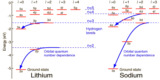
(the above picture is from the HyperPhysics website.)
The most significant deviations from the Bohr formula occur for the smallest l states in each orbital; these are precisely the states with wavefunctions that overlap significantly with the origin. These electrons can “see inside” the lower filled orbitals, and as a result are sensitive to the additional structure and stronger nuclear charge of the heavier elements.
Finally, we can also study the opposite limit r \rightarrow \infty. Once again assuming the potential is well-behaved, this time that V(r) \rightarrow 0 as r \rightarrow \infty, then the centrifugal contribution vanishes. If we have a bound state E<0, then the equation becomes \frac{d^2 u_E}{dr^2} = \frac{-2mE}{\hbar^2} u_E. We find decaying exponential behavior, u_E(r) \propto e^{-\kappa r}, where as usual \kappa = \sqrt{-2mE} / \hbar. Thus, for a bound state in any potential which vanishes at infinity and isn’t “too singular” at the origin, we know immediately what the asymptotic form looks like.
In fact, it’s often useful to “scale out” these asymptotic behaviors, and solve for the modified function w_{El}(\rho) = \rho^{-(l+1)} e^{\rho} u_{El}(\rho), leading to the modified differential equation \frac{d^2 w}{d\rho^2} + 2 \left( \frac{l+1}{\rho} - 1 \right) + \left[ \frac{V}{E} - \frac{2(l+1)}{\rho} \right] w = 0. This is the best setup to deal with the Coulomb potential.
12.4 Example: The isotropic harmonic oscillator
Now let’s move past generalities and actually solve a real Hamiltonian: we’ll study a version of the harmonic oscillator which is spherically symmetric, i.e. \hat{H} = \frac{\hat{\vec{p}}^2}{2m} + \frac{1}{2} m \omega^2 r^2. Once again, now that we’re dealing with more complicated differential equations it’s handy to rescale all our variables to be dimensionless. We make the replacements E = \frac{1}{2} \hbar \omega \lambda, \\ r = \sqrt{\frac{\hbar}{m \omega}} \rho, which gives for the radial equation \frac{d^2 u}{d\rho^2} - \frac{l(l+1)}{\rho^2} u(\rho) + (\lambda - \rho^2) u(\rho) = 0. Note that we can’t rewrite this in terms of the asymptotically rescaled function w(\rho), because one of the conditions is violated: the potential energy no longer vanishes as r \rightarrow \infty. We can still rescale to remove the short-distance asymptotic behavior, and anticipating the result I’ll include an exponential rescaling factor too: u(\rho) = \rho^{l+1} e^{-\rho^2 / 2} f(\rho). (I’m following Sakurai in the inclusion of the mysterious-looking exponential factor here. We could just as easily have only scaled out the \rho \rightarrow 0 behavior; the resulting differential equation is a little more difficult to deal with using the technique we’re about to introduce. Plus, we know from the form of our solutions to the 1-D harmonic oscillator that an exponential dependence of this form is likely to show up.)
With this substitution, we arrive at the differential equation \rho \frac{d^2 f}{d\rho^2} + 2[(l+1) - \rho^2] \frac{df}{d\rho} + [\lambda - (2l+3)] \rho f(\rho) = 0. This might not look any nicer than the equation we started with, but it is actually an improvement! Usually I just say “this is a standard differential equation” and tell you that the solution is some special function, but let’s actually work out the solution this time. Because all of the coefficients of the terms here involve small powers of \rho, the form of this equation suggests that we should try a power-series solution: f(\rho) = \sum_{k=0}^\infty a_k \rho^k. In fact, this assumption justifies the fact that we’ve pulled out the e^{-\rho^2/2}; as long as our series solution doesn’t diverge too badly at large \rho, the exponential suppression will win and ensure that u(\rho) \rightarrow 0 at infinity, as it should since the harmonic oscillator potential diverges at infinity.
Plugging back in, we have \sum_{k=0}^\infty k(k-1) a_k \rho^{k-1} + 2 \sum_{k=0}^\infty k a_k [(l+1) \rho^{k-1} - \rho^{k+1}] + [\lambda - (2l+3)] \sum_{k=0}^\infty a_k \rho^{k+1} = 0. If this is a valid solution to the differential equation, then the left-hand side must vanish for any value of \rho, which means that the coefficients of every power of \rho must independently be equal to zero. The \rho^0 term is quite simple: out of the four power series terms above, only the second series with k=1 gives a \rho^0 contribution, so we read off 2a_1 (l+1) \rho^0 = 0 which tells us that a_1 = 0. To continue, it’s useful to shift the sums so that we can write all of the terms using the same order in \rho: \sum_{k=0}^\infty \rho^k \left\{ k(k+1) a_{k+1} + 2(k+1) (l+1) a_{k+1} - 2(k-1) a_{k-1} + [\lambda - (2l+3)] a_{k-1} \right\} = 0. or, order by order, [(k+1)(k+2) + 2(l+1)(k+2)] a_{k+2} = [2k - \lambda + (2l+3)] a_k. This is a recursion relation for the power series coefficients: a_{k+2} = \frac{2k+2l+3-\lambda}{(k+2)(k+2l+3)} a_k. Since we already found that a_1 = 0, this immediately tells us that all of the odd terms in the power series are zero. We can also quickly find the asymptotic form of our series; in the limit k \rightarrow \infty, we have \lim_{k \rightarrow \infty} \frac{a_{k+2}}{a_k} = \frac{2}{k} \equiv \frac{1}{q}, where now since k was an even integer, q \equiv k/2 is any integer. Returning to the power series, f(\rho) \rightarrow \sum_q \frac{1}{q!} (\rho^2)^q \propto e^{\rho^2}. This reveals that we haven’t successfully scaled out the asymptotic large-\rho behavior from our function; plugging back in, we will find that u(\rho) itself, and thus R(\rho), will diverge exponentially for large \rho, which gives us an unnormalizable wavefunction. The only way out is for the power series to terminate at some value, i.e. for some k we must have 2k + 2l + 3 - \lambda = 0. This is just what we should have expected to find, namely a quantization condition for the bound-state energy (which is buried in \lambda, remember.) Converting back from the dimensionless \lambda to the energy, we have the result E_{ql} = \left( 2q + l + \frac{3}{2} \right) \hbar \omega = \left( N + \frac{3}{2} \right) \hbar \omega, where n = 2q + l. N here is sometimes referred to as the principal quantum number.
We observe a large amount of degeneracy here, i.e. for any given N there are several choices of q and l which will lead to the same energy. N=1 requires q=0, l=1; this is really three identical states since we’ve neglected the label m=-1,0,1. For N=2 we can have either q=0, l=2 (five states) or q=1, l=0 (one state), for a total of six. Even N implies even l, and vice-versa, so the eigenstates of N have definite parity, even for even N and odd for odd N.
Just like the one-dimensional simple harmonic oscillator, this spherically symmetric version appears often in approximate models of more complicated physical systems. The “shell model” of nuclear structure is a particularly widely-used example of such a model.
You might have noticed that after all of our hard work with the power series, our solution for the energy eigenvalues ended up being very simple. In fact, for this particular problem we made life harder for ourselves in some ways by using spherical coordinates at all, because we could have written the isotropic potential in the form V(\vec{r}) = \frac{1}{2} m \omega^2 (\hat{x}{}^2 + \hat{y}{}^2 + \hat{z}{}^2) So the isotropic harmonic oscillator is nothing more than a sum over three independent harmonic oscillators in the x,y,z directions, and we have E = \left( n_x + \frac{1}{2} + n_y + \frac{1}{2} + n_z + \frac{1}{2} \right) \hbar \omega = \left( N + \frac{3}{2} \right) \hbar \omega. The degeneracy of states is, of course, independent of what coordinate system we use; you can verify that explicitly for the first few values of N.
On the subject of degeneracy, it’s interesting to note that for a given energy level E_n, we can have very different quantum numbers for radial excitation (q) and orbital excitation (l) of the system; it’s somewhat unexpected that radial and orbital excitations would both contribute (up to a factor of 2) equally to the overall energy of the state. This is an example of an “accidental” degeneracy, where two very different sources of energy nevertheless give identical contributions. In the hydrogen atom, the energy levels of the electron look very similar to what we’ve written, E_{ql} = \frac{1}{2} mc^2 \frac{\alpha^2}{(q+l+1)^2} = \frac{-13.6\ \textrm{eV}}{n^2}, i.e. the principal quantum number of hydrogen is n = q + l + 1, and we again find accidental degeneracy.
Despite the name, each of these degeneracies are not really “accidental”; a better word might be “hidden”. They occur because of a hidden symmetry of the Coulomb and harmonic oscillator potentials that we haven’t taken into account, based on something known as the Laplace-Runge-Lenz vector, which you may have seen in an advanced derivation of Kepler’s laws or something like that. This is a fairly arcane and specialized example of a symmetry that is special to two-body inverse-square-law problems, so I won’t go into any further detail on it here.
We could, at this point, set up the two-body problem and solve the radial equation with the Coulomb potential, in order to find the spectrum and wavefunctions of the hydrogen atom. This is a very standard textbook problem, but unfortunately it’s also not a great example: hydrogen is a very special system, and is one of the very few atomic systems that can be solved exactly, so it admits some special techniques that won’t help you to solve for, say, the energies of a helium atom. As a result, I won’t be going through the basic hydrogen solution in class; you will find a thorough treatment in almost any quantum mechanics textbook. Instead, we’ll consider a number of interesting atomic effects that can be understood through spin and angular momentum.