3 The two-state system
The Stern-Gerlach experiment as we have considered it is an especially nice example, because it can be described as a two-state system. A two-state system in quantum mechanics is simply a system for which only two states are needed to construct a complete basis, i.e. the Hilbert space is two-dimensional.
Like the harmonic oscillator, the two-state system is ubiquitous in physics because it provides a good approximate description to a lot of realistic systems, and because we can solve it completely and exactly. A few other places you will encounter two-state quantum systems include:
- Lasers: the key idea of a laser, stimulated emission, is best described with a two-state system. Even if we are interested in more realistic and complicated lasers with more states, we can use multiple two-state system approximations to study individual processes (pumping, spontaneous emission, stimulated emission.)
- Atomic transitions: either in isolation or interacting with an electromagnetic field, a single transition can be approximated by a two-state system, and in many situations one transition is dominant. Nuclear magnetic resonance imaging is one example of many here.
- Neutrinos are elementary particles which, even in vacuum, can oscillate from one species into another. (Here you can object because this should obviously be a three-state system, but in practice in particle physics, we can and do generally describe the oscillations in terms of a set of two-state systems!)
- Quantum computers are built from a variety of two-state systems, which in that context are also known as qubits.
Basically everything we’re about to go through can be applied to any of these systems, but for concreteness, I’ll make some references to Stern-Gerlach as the motivating example. Our starting point is the general state
\ket{\psi} = \alpha \ket{\uparrow} + \beta \ket{\downarrow}
which again, must be normalized, giving the restriction |\alpha|^2 + |\beta|^2 = 1. Applying normalization leaves three real numbers as free parameters. Let’s parameterize them in the following form: \ket{\psi} = e^{i\zeta} \left[\cos(\theta/2) \ket{\uparrow} + \sin(\theta/2) e^{i \phi} \ket{\downarrow} \right]. Because of the overall phase in front (which can flip the sign of the whole state), we can cover all possible values with \theta \in [0,\pi) and \phi \in [0, 2\pi). The number \zeta here is a global phase: we can simply absorb it without changing any of the physics. Basically, this is because only squared amplitudes are physical. Suppose we have a second arbitrary state \ket{\psi'}. Then the inner product of the two states is \left\langle \psi' | \psi \right\rangle = e^{i(\zeta - \zeta')} \left[ \cos(\theta'/2) \cos(\theta/2) + \sin(\theta'/2) \sin(\theta/2) e^{i(\phi-\phi')} \right].
But the state overlap itself is not observable - only the square of the overlap |\left\langle \psi' | \psi \right\rangle|^2 is, through Born’s rule (postulate 4.) The phases \phi and \phi' matter because they will survive in the square, but \zeta and \zeta' vanish from the probability no matter what.
Don’t let the irrelevance of the global phase \zeta lull you into thinking that phases don’t matter in quantum mechanics. The relative phase of the two basis states within \ket{\psi}, \phi - \phi', is most certainly observable and will appear in the probabilities computed through Born’s rule.
Likewise, the state e^{-i\zeta} \ket{\psi} is not the same as \ket{\psi} in general! Again, from above, we can’t just take our basis state \ket{\downarrow} and rephase it - it will change the answer. The key here is that \zeta is a phase being applied to both of our basis states at once, which ensures that it will always end up being discarded when we apply Born’s rule. Always be careful when “throwing out” phases in quantum mechanics calculations; if in doubt, a good rule of thumb to remember is that you can always apply an arbitrary phase to your quantum state at the end of any given calculation, but it may not be safe to do so beforehand.
In fact, even overall phases like \zeta can become physically significant if they are not just constants, but depend on space or time. We’ll see more about this when we study gauge symmetry later on, where there will be very deep connections between these phases and electromagnetism!
Based on the above, we only need two real numbers to fully describe an arbitrary state, \theta and \phi. As suggested by the use of angles, we can visualize this nicely as a point on the surface of a sphere (called the Bloch sphere after the physicist of the same name). The choice above corresponds to putting the states \ket{\uparrow} and \ket{\downarrow} at the north and south poles respectively:
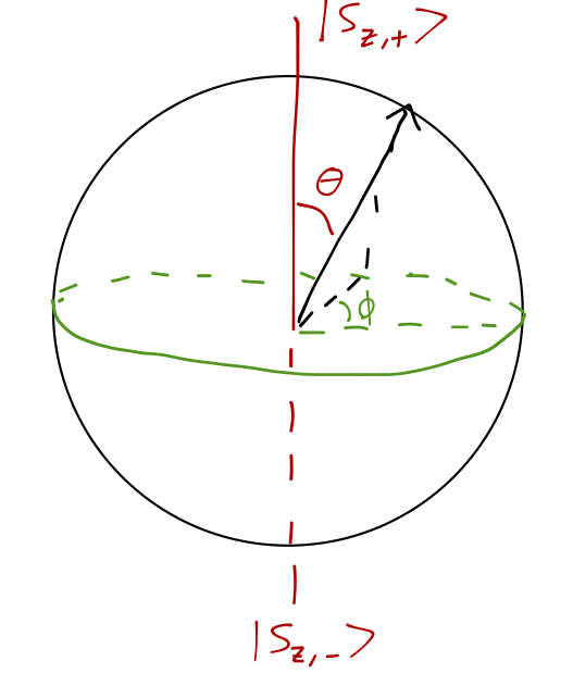
\ket{\psi} = \cos(\theta/2) \ket{\uparrow} + \sin(\theta/2) e^{i \phi} \ket{\downarrow}
I should note in passing that only needing two real numbers is unique to the two-state system, i.e. for a three-state system, we would need four real parameters (three complex numbers, minus one normalization condition, minus one global phase.)
3.1 Two-state observables; Pauli matrices
Now that we have a general description of quantum states, we need to think about observables. By postulate 2, any observable is Hermitian, which means we’re interested in all possible Hermitian two-by-two matrices. Here is the most general such matrix, written in terms of some real numbers w,x,y,z:
\hat{O} = \left( \begin{array}{cc} w+z & x-iy \\ x+iy & w-z \end{array}\right). Here we’ve just applied Hermiticity (\hat{O}^\dagger = \hat{O}), which tells us the diagonal entries are real (but can be different), while the off-diagonals must be complex conjugates of one another. I have written this in a suggestive form to allow me to split it into a sum over four “basis” matrices: \hat{O} = w \hat{1} + x \hat{\sigma}_x + y \hat{\sigma}_y + z \hat{\sigma}_z.
The operator \hat{1} is just the identity matrix, while the other three are a special set of matrices known as the Pauli matrices which we will encounter often:
The Pauli matrices are defined as follows: \begin{aligned} \hat{\sigma}_x &\equiv \left( \begin{array}{cc} 0 & 1 \\ 1 & 0 \end{array}\right) \\ \hat{\sigma}_y &\equiv \left( \begin{array}{cc} 0 & -i \\ i & 0 \end{array}\right) \\ \hat{\sigma}_z &\equiv \left( \begin{array}{cc} 1 & 0 \\ 0 & -1 \end{array}\right). \end{aligned}
(Note that some references will label these as \hat{\sigma}_{1,2,3} instead.)
The Pauli matrices have some very useful properties which are straightforward to check:
They square to the identity: \hat{\sigma}_i^2 = \hat{1}.
They obey the commutation relations
\begin{aligned} [\hat{\sigma}_x, \hat{\sigma}_y] &= 2i \hat{\sigma}_z \\ [\hat{\sigma}_x, \hat{\sigma}_z] &= -2i \hat{\sigma}_y \\ [\hat{\sigma}_y, \hat{\sigma}_z] &= 2i \hat{\sigma}_x \\ \end{aligned}
or more compactly, [\hat{\sigma_i}, \hat{\sigma_j}] = 2i \epsilon_{ijk} \hat{\sigma_k} where \epsilon_{ijk} is the Levi-Civita symbol (see below if you’re not familiar with it.)
- They obey the anti-commutation relation \{\hat{\sigma}_i, \hat{\sigma}_j\} = 2\delta_{ij} \hat{1}.
In case you aren’t familiar with it, the Levi-Civita symbol \epsilon_{ijk} is an object whose entries are either 1, -1, or 0, and it is totally antisymmetric under exchange of its indices. This tells you immediately what the whole tensor looks like, once we fix the convention that \epsilon_{xyz} = 1:
- \epsilon_{ijk} = 0 if any of i,j,k are the same;
- All other entries are obtained by counting how many times we exchanged two indices from \epsilon_{xyz} to get to them. For example, \epsilon_{xzy} is a single exchange, and so it is -1; \epsilon_{zxy} requires a second exchange and it is equal to +1.
So we find that in a two-state system, the operator for any physical observable can be built from a combination of the Pauli matrices and the identity matrix. Of course, this is only one “basis” - we could have chosen other matrices. I’ve used the Pauli matrices specifically because in systems involving spin, like the Stern-Gerlach system, they correspond naturally to physical observations of spin.
3.2 Stern-Gerlach as a two-state system
Now that we have the mathematical ingredients - states on the Bloch sphere and observables built from Pauli matrices - let’s see how they map concretely onto our example Stern-Gerlach experiment. We’ll adopt the usual convention and identify our basis states \ket{\uparrow} and \ket{\downarrow} as the corresponding outputs from SG(\hat{z}). As we discussed, these outputs correspond to values of \pm \hbar/2 for the \hat{z}-component of the spin of the atoms, \hat{S}_z. From the postulates, this means that \ket{\uparrow}, \ket{\downarrow} as measurement outcomes are eigenstates of \hat{S}_z, and we also know the eigenvalues:
\hat{S}_z \ket{\uparrow} = +\tfrac{\hbar}{2} \ket{\uparrow}; \\ \hat{S}_z \ket{\downarrow} = -\tfrac{\hbar}{2} \ket{\downarrow}.
Looking back at our Pauli matrices, which have been defined in suggestive notation, we can immediately see that in matrix form, \hat{S}_z = \frac{\hbar}{2} \left( \begin{array}{cc} 1 & 0 \\ 0 & -1 \end{array}\right) = \frac{\hbar}{2} \hat{\sigma}_z. (Convince yourself that the off-diagonal entries are zero, either mathematically or from the experiment!)
So far, so good; now let’s consider the other spin directions. Here’s one of the sequential configurations we looked at before:
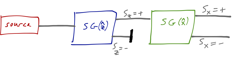
On the final screen to the right, we again find two spots of equal intensity, corresponding to S_x = \pm \hbar/2. We also know that the outputs at the final screen are now eigenstates of \hat{S}_x and not of \hat{S}_z. Let’s denote the x-direction eigenstates as \ket{S_{x,+}} and \ket{S_{x,-}}. Then from Born’s rule, |\left\langle \uparrow | S_{x,+} \right\rangle| = |\left\langle \uparrow | S_{x,-} \right\rangle| = \frac{1}{\sqrt{2}}, and similarly if we input \ket{\downarrow}, which tells us what the eigenkets of \hat{S_x} look like: \ket{S_{x,+}} = \frac{1}{\sqrt{2}} \ket{\uparrow} + \frac{1}{\sqrt{2}} e^{i \delta_1} \ket{\downarrow}, \\ \ket{S_{x,-}} = \frac{1}{\sqrt{2}} \ket{\uparrow} - \frac{1}{\sqrt{2}} e^{i \delta_1} \ket{\downarrow}. Actually, there is one more piece of information I’ve used here, which is that the kets are orthogonal: \left\langle S_{x,+} | S_{x,-} \right\rangle = 0. Once again, we can argue this mathematically (eigenstates with distinct eigenvalues are always orthogonal) or physically (we know that the probability of measuring S_x = - from the S_x = + beam is zero.)
Let’s put our work so far in terms of the Bloch sphere. The eigenstates of \hat{S}_z, \ket{\uparrow}, \ket{\downarrow}, exist at the north and south poles. Then the \hat{S}_x states we just found exist somewhere on the equator, with \theta = \pi/2, and they are also at equal and opposite points around the sphere (their phases \phi_{\pm} differ by exactly \pi.) But without further information, we can’t fix the final unknown phase \delta_1.
Is there any more information we can use to fix the extra phase factor? Remember that we can orient the S-G device in a third independent direction, along the y axis. In fact, we know that there is no difference between performing the sequential S-G experiment in the order z-x-z or z-y-z, which means that the construction of the \hat{S_y} eigenstates is basically identical, i.e. \ket{S_{y,+}} = \frac{1}{\sqrt{2}} \ket{\uparrow} + \frac{1}{\sqrt{2}} e^{i \delta_2} \ket{\downarrow}, \\ \ket{S_{y,-}} = \frac{1}{\sqrt{2}} \ket{\uparrow} - \frac{1}{\sqrt{2}} e^{i \delta_2} \ket{\downarrow}. We assign the \hat{S}_y eigenstates their own phase \delta_2, which can be different from \delta_1. In fact, it has to be different because we have another experimental input: we can perform the same sequential experiment using only x and y-direction S-G devices, which means that |\left\langle S_{y,\pm} | S_{x,+} \right\rangle| = |\left\langle S_{y,\pm} | S_{x,-} \right\rangle| = \frac{1}{\sqrt{2}}. Now we multiply out the kets we found above. For example, the product between both “+” components gives |\left\langle S_{y,+} | S_{x,+} \right\rangle| = \frac{1}{2} \left( 1 + e^{i(\delta_1 - \delta_2)} \right). Looking at all four products, we find two distinct equations, \left|1 \pm e^{i(\delta_1 - \delta_2)}\right| = \sqrt{2} the only solutions to which are \delta_1 - \delta_2 = \pm \frac{\pi}{2}. Going back to the Bloch sphere, the final answer is more or less what you might have guessed: the states are maximally “spaced out”. The \hat{S}_x and \hat{S}_y eigenstates come in pairs on equal and opposite sides of the equator, and they are rotated \pi/2 relative to each other, so the four states form an equally-spaced ring around the equator. Note that this immediately means that, as I mentioned in the first lecture, it is impossible to make all of the kets real at the same time - we need complex numbers for even this very simple quantum system!
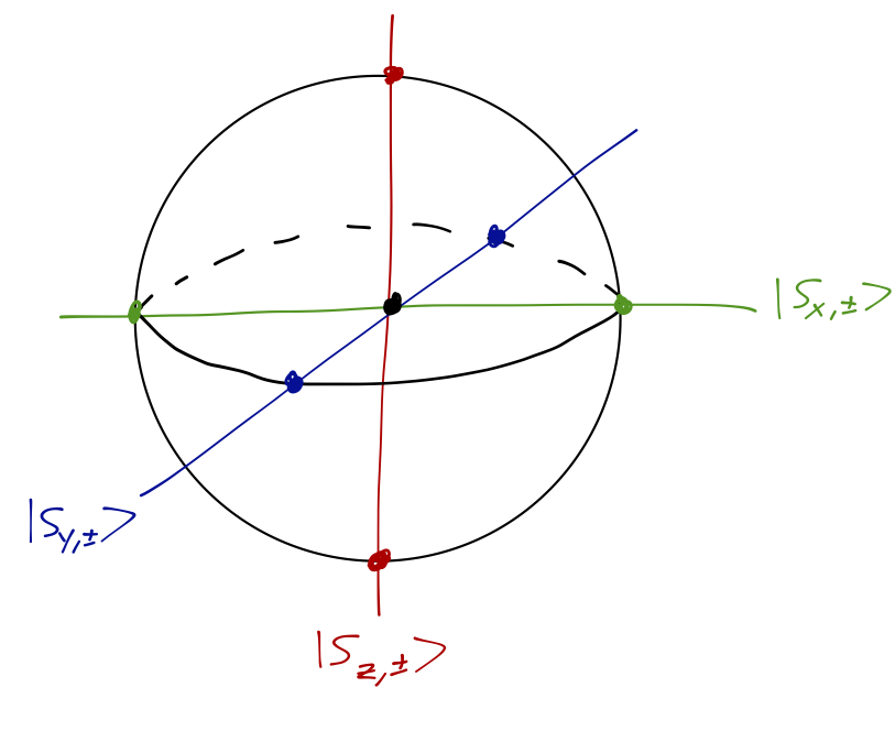
There are still, apparently, two ambiguities left in our total specification of the system: the value of \delta_1, and the sign of \delta_1 - \delta_2. We haven’t developed the machinery to consider symmetries, in particular changes in coordinate systems, just yet, but both of these choices amount to a choice of coordinates. It’s easiest to see this geometrically from the Bloch sphere: our \hat{S_z} eigenstates are at the poles, and \hat{S_x} and \hat{S_y} exist on the equator, equally spaced and separated by \phi = \pi/2.
It’s clear from the picture that choosing \delta_1 just amounts to choosing the position of the second coordinate axis (we’ve already forced one axis through the \hat{S_z} states on the poles.) The choice of sign for \delta_1 - \delta_2 is a convention, namely whether we are working in a left-handed or right-handed coordinate system. We’ll use standard right-handed coordinates in this class, which if we take \delta_1 = 0 gives \delta_2 = \pi/2 as the correct choice.
With our conventions fixed, we now know all of the spin-operator eigenstates: \ket{S_{x,+}} = \frac{1}{\sqrt{2}} \ket{\uparrow} + \frac{1}{\sqrt{2}} \ket{\downarrow}, \\ \ket{S_{x,-}} = \frac{1}{\sqrt{2}} \ket{\uparrow} - \frac{1}{\sqrt{2}} \ket{\downarrow}, \\ \ket{S_{y,+}} = \frac{1}{\sqrt{2}} \ket{\uparrow} + \frac{i}{\sqrt{2}} \ket{\downarrow}, \\ \ket{S_{y,-}} = \frac{1}{\sqrt{2}} \ket{\uparrow} - \frac{i}{\sqrt{2}} \ket{\downarrow}.
Knowing the eigenstates and eigenvalues from above is all we need to build the corresponding operators; find \hat{S}_x and \hat{S}_y.
Answer:
We begin with \hat{S}_x. If we know the eigenvectors, we can build a matrix from outer products: \hat{S_x} = \frac{\hbar}{2} \ket{S_{x,+}} \bra{S_{x,+}} - \frac{\hbar}{2} \ket{S_{x,-}} \bra{S_{x,-}} \\ = \frac{\hbar}{4} \left( (\ket{\uparrow} + \ket{\downarrow}) (\bra{\uparrow} + \bra{\downarrow}) - (\ket{\uparrow} - \ket{\downarrow}) (\bra{\uparrow} - \bra{\downarrow}) \right) \\ = \frac{\hbar}{4} \left( 2 \ket{\uparrow} \bra{\downarrow} + 2 \ket{\downarrow} \bra{\uparrow} \right) \\ = \frac{\hbar}{2} \left( \begin{array}{cc} 0 & 1 \\ 1 & 0 \end{array}\right).
For \hat{S_y}, everything is very similar, but the complex conjugation on the bras gives some extra signs. Going slowly: \hat{S_y} = \frac{\hbar}{2} \ket{S_{y,+}} \bra{S_{y,+}} - \frac{\hbar}{2} \ket{S_{y,-}} \bra{S_{y,-}} \\ = \frac{\hbar}{4} \left( (\ket{\uparrow} + i\ket{\downarrow}) (\bra{\uparrow} - i\bra{\downarrow}) - (\ket{\uparrow} - i\ket{\downarrow})(\bra{\uparrow} + i\bra{\downarrow}) \right) \\ = \frac{\hbar}{4} \left( -2i \ket{\uparrow} \bra{\downarrow} + 2i \ket{\downarrow} \bra{\uparrow} \right) \\ = \frac{\hbar}{2} \left( \begin{array}{cc} 0 & -i \\ i & 0 \end{array}\right).
No surprise that we ended up with the other two Pauli matrices!
You can also double-check the algebra here by going backwards: computing the eigenvectors and eigenvalues of the matrices we obtained in the usual way, and making sure we reconstruct the vectors that we started with.With the phases all fixed, we have for our final set of three operators exactly just the Pauli matrices times \hbar/2:
\hat{S}_x = \frac{\hbar}{2} \left( \begin{array}{cc} 0 & 1 \\ 1 & 0 \end{array} \right) = \frac{\hbar}{2} \hat{\sigma}_x \\ \hat{S}_y = \frac{\hbar}{2} \left( \begin{array}{cc} 0 & -i \\ i & 0 \end{array} \right) = \frac{\hbar}{2} \hat{\sigma}_y \\ \hat{S}_z = \frac{\hbar}{2} \left( \begin{array}{cc} 1 & 0 \\ 0 & -1 \end{array} \right) = \frac{\hbar}{2} \hat{\sigma}_z.
3.3 Commutation and compatible observables
As I hinted before, the commutator is a particularly interesting property to look at between operators. We’ve seen in the Stern-Gerlach experiment that the order in which we apply measurements matters: for example, projecting upper components in the order S_{z,+}, S_{x,+}, S_{z,-} gives a non-zero signal, but reversing the order to S_{z,+}, S_{z,-},S_{x,+} does not.
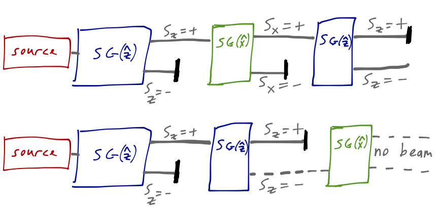
This non-commutation of measurements is easy to see in the operator formalism. We know that when we make a measurement, the state of the system collapses into one of the eigenstates of whatever operator we observe, for example \hat{S_z} \ket{\psi} \rightarrow \pm \frac{\hbar}{2} \ket{S_{z,\pm}}. Clearly if we perform the same measurement again (ignoring time evolution of the state itself, which we’ll get to), Born’s rule tells us that we find the same eigenvalue with probability 1. We can see this clearly in the sequential case sketched above with two SG(\hat{z}) measurements in a row.
However, if we perform a different measurement, we won’t get a guaranteed outcome anymore. Moreover, we can see that the order of measurement matters, from the sketch above: \hat{S_x} \hat{S_z} \ket{\uparrow} \neq \hat{S_z} \hat{S_x} \ket{\uparrow} \Rightarrow [\hat{S_x}, \hat{S_z}] \ket{\uparrow} \neq 0. In other words, experimentally, the observables \hat{S_x} and \hat{S_z} do not commute - and in fact, this is true for any state, not just \ket{\uparrow}. From our work above, you can easily verify that this is true algebraically, simply because the commutator [\hat{\sigma}_x, \hat{\sigma}_z] \neq 0.
What if we had two operators that did commute with each other? In general, if [\hat{A}, \hat{B}] = 0, we say that \hat{A} and \hat{B} are compatible operators. But let’s think about what that implies: we know for any state \ket{\psi}, that \hat{A} \hat{B} \ket{\psi} = \hat{B} \hat{A} \ket{\psi}. Now suppose that \ket{\psi} is an eigenstate of \hat{A}, call it \ket{a}. If we measure \hat{A} first, then we get outcome a with 100% probability. But because the operators commute, if we measure \hat{B} first, we still get outcome a for \hat{A} with 100% probability. You can convince yourself that the only way this can be true is if the eigenstates \ket{b} of \hat{B} are also eigenstates of \hat{A}, and vice-versa: so we can label all of the measurement outcomes as \ket{a,b}. Algebraically, this is the statement that \hat{A} and \hat{B} are simultaneously diagonalizable - we can find a basis of states that are eigenstates of both at once.
For those who are more mathematically inclined, here’s a quick proof of the statement above with some assumptions. If the eigenvalues of \hat{A} are non-degenerate, then in the basis of eigenkets \{ \ket{a}\}, a compatible operator \hat{B} is represented by a diagonal matrix. (Obviously, so is \hat{A}.) This is straightforward to see: \bra{a_j} [\hat{A}, \hat{B}] \ket{a_i} = \bra{a_j} (\hat{A} \hat{B} - \hat{B} \hat{A}) \ket{a_i} \\ = \sum_{k} \bra{a_j} \hat{A} \ket{a_k} \bra{a_k} \hat{B} \ket{a_i} - a_i \bra{a_j} \hat{B} \ket{a_i} \\ = \sum_{k} a_k \delta_{jk} \bra{a_k} \hat{B} \ket{a_i} - a_i \bra{a_j} \hat{B} \ket{a_i} \\ = (a_j - a_i) \bra{a_j} \hat{B} \ket{a_i} = 0. Since we assumed the eigenvalues of \hat{A} are non-degenerate, then if i \neq j the matrix element of \hat{B} is zero. So \hat{B} is diagonal.
Dealing with the degenerate case, where there can be eigenvalues of \hat{A} which appear repeatedly, is more complicated - but it can be done, and it is in fact generally true that if [\hat{A}, \hat{B}] = 0, there exists a basis in which the operators are simultaneously diagonalized. Although I won’t prove it, this also goes the other way: simultaneously diagonalizable operators must always commute with each other.
We’ll come back to a more general discussion of compatible operators and simultaneous diagonalization later on. For the two-state system, things are very constrained: we know that none of the spin-component operators \hat{S_x}, \hat{S_y}, \hat{S_z} commute with one another. The only thing that can commute is the identity operator \hat{1}, and in fact this does correspond to a physical observable, which is the square of the spin vector: \hat{\mathbf{S}}{}^2 \equiv \hat{S_x}{}^2 + \hat{S_y}{}^2 + \hat{S_z}{}^2 = \frac{3}{4} \hbar^2 \hat{1}, where we’ve used the properties of the Pauli matrices to show that this operator is proportional to the identity operator. Clearly, this implies that [\hat{\mathbf{S}}{}^2, \hat{S_i}] = 0 and the eigenstates of any of the \hat{S_i} are also eigenstates of \hat{\mathbf{S}}{}^2. But this is trivial in this case: the identity operator always gives us the same outcome for any state. As we will see later, for systems with higher spin \hat{\mathbf{S}}{}^2 will become more interesting.
3.4 The uncertainty relation
If two observables are not compatible, [\hat{A}, \hat{B}] \neq 0, then they do not have simultaneous eigenstates: we can’t precisely know the values of both observables simultaneously. What we can do is make statistical statements; given an ensemble in some state \ket{\psi} and many repeated trials, we can determine the expectation values \left\langle \hat{A} \right\rangle and \left\langle \hat{B} \right\rangle.
But it turns out that even when we’re willing to back off to statistical measurements of an ensemble, there is still a fundamental limit on how precisely we can predict the outcomes of incompatible observables. You have seen this before in the form of the Heisenberg uncertainty principle for momentum and position of a particle. Here we consider a more general inequality known as the uncertainty relation.
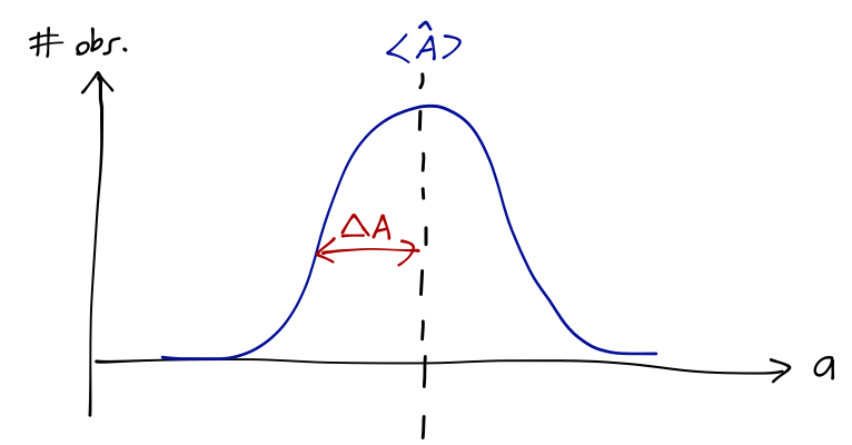
Following Sakurai, we define an operator \Delta \hat{A} \equiv \hat{A} - \left\langle \hat{A} \right\rangle which measures the residual difference between the outcome of \hat{A} and the expected mean. The expectation value of the square of this difference is called the variance or the dispersion: (\Delta A)^2 \equiv \left\langle (\Delta \hat{A})^2 \right\rangle = \left\langle \left(\hat{A}^2 - 2 \hat{A} \left\langle \hat{A} \right\rangle + \left\langle \hat{A} \right\rangle^2 \right) \right\rangle = \left\langle \hat{A}^2 \right\rangle - \left\langle \hat{A} \right\rangle^2. (Note that Sakurai doesn’t use the notation “(\Delta A)^2” for the variance, to avoid confusion with the operator \Delta \hat{A}; since I’m using hat notation for operators, we can use the more conventional notation for the variance.)
This dispersion measures how widely dispersed the results of measuring \hat{A} will be over many trials. In fact, by the central limit theorem, if we repeat our experiment an enormous number of times the distribution will be a Gaussian, centered at \left\langle \hat{A} \right\rangle and with 68% of the observations within one standard deviation \Delta A of \left\langle \hat{A} \right\rangle.
We know that there are some experiments for which the dispersion will be zero; if we prepare a pure eigenstate \ket{a} of \hat{A}, then we will always measure the same eigenvalue a. However, for a more general state there will be some dispersion. In particular, even if our system is in an eigenstate of \hat{A}, we might expect to find some dispersion if we measure an incompatible observable \hat{B}. For example, if we go back to our Stern-Gerlach system and prepare an eigenstate \ket{\uparrow} of \hat{S_z}, then \Delta S_z = 0, but if we try to measure \hat{S_x}, we find that \Delta S_x = \sqrt{\left\langle \hat{S_x}^2 \right\rangle - \left\langle \hat{S_x} \right\rangle^2} = \frac{\hbar}{2}. If we choose a different state, the dispersions of \hat{S_x} and \hat{S_z} will be different, but they can never both be made arbitrarily small; there is a limit on the combination of the two.
For any state and any two observables \hat{A} and \hat{B}, their variances must satisfy the uncertainty relation,
(\Delta A) (\Delta B) \geq \frac{1}{2} \left| \left\langle [\hat{A}, \hat{B}] \right\rangle\right|.
Let’s prove this inequality. Our starting point is the Cauchy-Schwarz inequality: if we let \ket{\alpha} = \Delta \hat{A} \ket{\psi} \\ \ket{\beta} = \Delta \hat{B} \ket{\psi} where \ket{\psi} is arbitrary, then the inequality gives us \left\langle \alpha | \alpha \right\rangle \left\langle \beta | \beta \right\rangle \geq |\left\langle \alpha | \beta \right\rangle|^2 \\ \Rightarrow \bra{\psi}(\Delta \hat{A})^2 \ket{\psi} \bra{\psi} (\Delta \hat{B})^2 \ket{\psi} \geq |\bra{\psi} (\Delta \hat{A}) (\Delta \hat{B}) \ket{\psi}|^2. Now we’ll use a useful trick: we can rewrite the product of two operators like so, \Delta \hat{A} \Delta \hat{B} = \frac{1}{2} [\Delta \hat{A}, \Delta \hat{B}] + \frac{1}{2} \{ \Delta \hat{A}, \Delta \hat{B}\}. (If it’s not obvious this is true, expand out and convince yourself!) We know that the observables themselves are Hermitian, but what about the commutator and anti-commutator? Well, first notice that [\Delta \hat{A}, \Delta \hat{B}] = [\hat{A} - \left\langle \hat{A} \right\rangle, \hat{B} - \left\langle \hat{B} \right\rangle] = [\hat{A}, \hat{B}] since the commutator vanishes if either argument is a scalar. This commutator is anti-Hermitian: ([\hat{A}, \hat{B}])^\dagger = (\hat{A} \hat{B} - \hat{B} \hat{A})^\dagger \\ = \hat{B}^\dagger \hat{A}^\dagger - \hat{A}^\dagger \hat{B}^\dagger \\ = \hat{B} \hat{A} - \hat{A} \hat{B} \\ = - [\hat{A}, \hat{B}]. Just like the expectation value of any Hermitian operator is real, that of an anti-Hermitian operator is purely imaginary. On the other hand, it’s easy to show that the anticommutator \{\Delta \hat{A}, \Delta \hat{B}\} is in fact Hermitian. So we’ve rewritten the object inside the absolute value above as a real part and an imaginary part, which means that the absolute value is just the sum of the squares: \left|\left\langle \Delta \hat{A} \Delta \hat{B} \right\rangle\right|^2 = \frac{1}{4} \left| \left\langle [\hat{A}, \hat{B}] \right\rangle \right|^2 + \frac{1}{4} \left| \left\langle \{\Delta \hat{A}, \Delta \hat{B}\} \right\rangle \right|^2 Since the anticommutator term is always positive, this is always greater than or equal to \frac{1}{4} \left| \left\langle [\hat{A}, \hat{B}] \right\rangle \right|^2, so our proof is complete; taking the square root of both sides gives the form of the relation written above.
Coming back to the two-state system: for any two spin-component observables, we have [\hat{S}_i, \hat{S}_j] = \frac{\hbar^2}{4} [\hat{\sigma}_i, \hat{\sigma}_j] = \frac{\hbar^2}{4} (2i \epsilon_{ijk} \hat{\sigma}_k). So concretely, we see that for example, \Delta S_x \Delta S_z \geq \frac{1}{2} \left| \left\langle [\hat{S}_x, \hat{S}_z] \right\rangle \right| = \frac{1}{4} \left| \left\langle \hat{S_y} \right\rangle \right|. As we saw above, it is possible to have zero uncertainty on one of the measurements: if we prepare an eigenstate of \hat{S_z} like \ket{\uparrow}, then \Delta S_z = 0. This doesn’t violate the uncertainty relation, because in that particular state \left\langle \hat{S_y} \right\rangle = 0 as well. But eigenstates are special, and since \hat{S}_x and \hat{S}_z don’t commute, it turns out to be impossible to also have \Delta S_x = 0 at the same time. If we insist on building states that are not eigenstate of either \hat{S}_x or \hat{S_z}, then both variances will be non-zero, but we will find that the uncertainty relation limits how we can construct such a state.