18 Identical particles
One subtlety that we have completely ignored so far in our discussion of multi-particle quantum systems is what to do when some of our particles are identical to each other, for example, if we want to study the helium atom in which we have two orbital electrons. There is no way to tell one electron apart from another, since they are elementary particles, hence “identical”.
Of course, to do a theoretical calculation, we’re always free to label our particles: in the example of helium we can label one of the electrons as “1” and the other as “2”. Although our choice of labels “1” and “2” is arbitrary, once we decide on a label we can consistently follow that particle along its entire trajectory for all time. If we were doing classical mechanics, this would be the end of the story, possibly aside from exploiting the symmetry of exchanging label 1 with label 2 when finding our solution.
For quantum mechanics, however, the idea of assigning labels breaks down, simply because we can’t follow a specific particle’s trajectory. If we observe electron 1 and electron 2 both entering some localized region of space, and then observe two electrons leaving the same region of space, there is no way to tell which one is 1 and which is 2. Both of the following paths are possible, and cannot be distinguished even in principle:
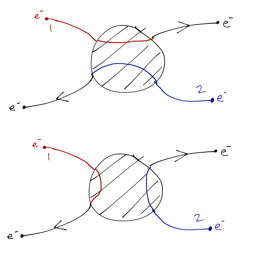
If we label the two distinct outgoing paths above as outcomes \alpha and \alpha', then the state after measurement collapses to \ket{\alpha} \ket{\alpha'} - except that we don’t know which particle is which, so there are two quantum states consistent with this outcome. In mathematical terms, the collapse of the state is only down to an arbitrary linear combination of these two states: \ket{\psi} \rightarrow c_1 \ket{\alpha}_1 \ket{\alpha'}_2 + c_2 \ket{\alpha'}_1 \ket{\alpha}_2. This leftover ambiguity is known as exchange degeneracy; it presents us with the puzzle that we cannot determine the state of our system completely, even if we measure every observable we can find! Fixing this will help us understand what a realistic solution for the helium atom looks like, and on top of that leads to a variety of interesting physical effects (the most famous of which is the Pauli exclusion principle which you already know from chemistry class.)
Many books use exchange degeneracy as the focus of deriving the symmetrization postulate. Here, I will instead focus on the operators instead of the states, although in the end we’ll have to return to considering the state itself anyway.
18.1 Permutation symmetry
Let’s be more concrete about what the idea of exchanging paths sketched above means mathematically. Suppose we have two identical particles, each of which carries a set of quantum numbers that we can label with the collective index \ket{\alpha}. They exist in two identical Hilbert spaces which we label as \mathcal{H}_1 and \mathcal{H}_2, so the overall Hilbert space is \mathcal{H} = \mathcal{H}_1 \otimes \mathcal{H}_2. If one of the particles (particle 1) is in state \ket{\alpha}_1, and the other (particle 2) is in state \ket{\alpha'}_2, then the overall state of the system is \ket{\alpha}_1 \ket{\alpha'}_2. This is not the same as the state \ket{\alpha'}_1 \ket{\alpha}_2 that would result from exchanging the two particles from each other; in fact, if these are basis states then those two options are orthogonal to one another, and thus perfectly distinguishable from each other. We’re not talking about measurements yet, this is just math, and from a mathematical point of view we can certainly distinguish which particle is in which state.
To proceed, let’s define an operator that will exchange particle labels for us, the permutation operator \hat{P}_{ij} (some references call this the “exchange operator” instead.) For a two-particle system, its definition is simple: we have
\hat{P}_{12} \ket{\alpha}_1 \ket{\alpha'}_2 = \ket{\alpha'}_1 \ket{\alpha}_2. There are some immediately obvious symmetry properties here. Clearly the order of the labels on the operator doesn’t matter, and applying it twice will take us back to our initial state: \hat{P}_{21} = \hat{P}_{12} \\ \hat{P}_{12}^2 = \hat{1} so that P_{12}^{-1} = P_{12}. These are all the same properties as parity, so we can recognize that this is the same symmetry group, \mathbb{Z}_2. How does the permutation operator act on observables? Since we have a bipartite Hilbert space again, the most general observable takes the form \hat{A}_1 \otimes \hat{B}_2; since we know the Hilbert spaces are identical, we know that \hat{B}_1 \otimes \hat{A}_2 is also a good operator. It’s straightforward to see that the permutation operator obeys \hat{P}_{12} (\hat{A}_1 \otimes \hat{B}_2) \hat{P}_{12} = \hat{B}_1 \otimes \hat{A}_2.
So far, all of the discussion is generic to any symmetry operator we might write down. But there is a key difference for the permutation operator, stemming from the observation we made above: because we can’t keep track of particle labels in quantum mechanics, it’s impossible to measure any quantity that depends on particle label. This means that we have to update one of our postulates again:
All physical observables correspond to Hermitian operators which are invariant under permutation symmetry for any identical particles.
This is simply a statement of the fact that if we can’t tell the particles apart, we can’t actually measure something like \hat{x}_1 \otimes \hat{1}_2 which would tell us the position of just particle 1, because we have no way of telling which particle that is. If we have two electrons and we try to measure the position of one of them, the operator we’re really measuring has to be instead \hat{x}_1 \otimes \hat{1}_2 + \hat{1}_1 \otimes \hat{x}_2. If we’re given a Hermitian operator \hat{O} which isn’t permutation invariant, we can always symmetrize it by using the permutation operator, so that \hat{O} + \hat{P}_{12} \hat{O} \hat{P}_{12} will be symmetric (and therefore something that we can measure.)
Another way to state this requirement is: in a system with two identical particles, when we go to make a measurement, it will be impossible to tell whether someone has switched them before we measured or not, because they are identical. If permuting before or after measurement gives the same answer, this means that we must have [\hat{O}, \hat{P}_{12}] = 0, which in turn implies that \hat{O} is invariant under the permutation symmetry. It’s also worth noting that since the Hamlitonian \hat{H} is itself a physical observable (we can measure energy), in any quantum system we must have [\hat{H}, \hat{P}_{12}] = 0, so that permutation symmetry is always a dynamical symmetry.
Because any \hat{O} and \hat{P}_{12} commute, they must admit a set of simultaneous eigenstates. Given the sets of other quantum numbers \alpha and \alpha', there are two different eigenstates of permutation that we can construct, \ket{\psi_S} = \frac{1}{\sqrt{2}} \left(\ket{\alpha}_1 \ket{\alpha'}_2 + \ket{\alpha'}_1 \ket{\alpha}_2 \right), \\ \ket{\psi_A} = \frac{1}{\sqrt{2}} \left(\ket{\alpha}_1 \ket{\alpha'}_2 - \ket{\alpha'}_1 \ket{\alpha}_2 \right). The symmetric combination \ket{\psi_S} has \hat{P}_{12} \ket{\psi_S} = +\ket{\psi_S}, while for the antisymmetric combination \hat{P}_{12} \ket{\psi_A} = -\ket{\psi_A}. These are the only options, since the eigenvalues of \hat{P}_{12} are \pm 1. Because the symmetry is preserved by all other operators we’re using to write the labels \alpha and \alpha', the total state can only be a combination of these two: \ket{\psi} = c_S \ket{\psi_S} + c_A \ket{\psi_A}, with |c_S|^2 + |c_A|^2 = 1. This has helped with the exchange degeneracy problem; if we consider the measurement of an operator \hat{O} in this state, since it must commute with \hat{P}_{12}, it’s easy to show that \bra{\psi_A} \hat{O} \ket{\psi_S} = 0, and so the expectation breaks down into two expectations, \left\langle \hat{O} \right\rangle = |c_S|^2 \left\langle \hat{O} \right\rangle_S + |c_A|^2 \left\langle \hat{O} \right\rangle_A. It is somewhat interesting that this looks exactly like a mixed state since no interference is possible, which leads into interesting philosophical discussions about the symmetrization postulate. But we don’t have to go any further with derivations, because at this point we are saved by the intervention of a deeper result.
In (3+1)-dimensional quantum mechanics, the behavior of a given particle under permutation symmetry is determined by its spin:
- All particles with integer spin (known as bosons) are symmetric under permutation (obeying “Bose-Einstein statistics”).
- All particles with half-integer spin (known as fermions) are anti-symmetric under permutation (obeying “Fermi-Dirac statistics”).
Spin-statistics resolves the remaining exchange degeneracy by telling us that in the arbitrary state above, we must either have c_S = 1 or c_A = 1, depending on what kind of particle the state is describing. Although spin-statistics can be proved rigorously in relativistic quantum field theory, as Feynman laments in his lectures (and still true many years later), there is no simple or intuitive explanation of the result. This means in his eyes (and mine) that we don’t fully understand the mechanism yet. Maybe one of you will find such an understanding!
Some quantum mechanics books state the result that either c_A = 1 or c_S = 1 in the form of a “symmetrization postulate” and add it to the list of other postulates of quantum mechanics, phrased in a different way, that only symmetrized or anti-symmetrized wavefunctions are physical. I think five postulates is enough; as the name implies, spin-statistics can be proved, not assumed, but it requires inclusion of relativistic effects (meaning working in quantum field theory, not just quantum mechanics.)
Experimentally, there are no exceptions to the spin-statistics theorem, no matter what the actual particle in question is. Photons, helium-4 atoms, carbon-12 nuclei, and J/\psi mesons are all bosons; electrons, neutrinos, protons, and helium-3 atoms are all fermions. As I’ve emphasized with my lists here, the term “particle” in the spin-statistics theorem does not refer only to elementary particles. The carbon-12 nucleus is a composite bound state of 6 protons and 6 neutrons. All of these nucleons are themselves fermions, and the wavefunction of the overall carbon-12 nucleus is certainly antisymmetric under exchange of two protons. Nevertheless, the carbon-12 nucleus itself is a boson; if we are studying a system consisting of many carbon-12 nuclei, then the wavefunction of the overall system is symmetric under exchange of two nuclei. As long as we’re only asking questions about the system of carbon-12 nuclei that don’t depend on their internal structure, then they are identical and act as bosons.
The famous Pauli exclusion principle is an immediate consequence of the spin-statistics theorem and the permutation symmetry we’ve outlined. Two electrons cannot exist in the same state simultaneously, because that would correspond to the state \ket{\alpha}_1 \ket{\alpha}_2, which is symmetric; as fermions, the electron wavefunction must be antisymmetric under exchange.
If you’re paying very close attention, you’ll notice that I specified “3+1 dimensions” in the spin-statistics theorem above. This is because in lower-dimensional systems, in particular systems with two spatial dimensions, there is another possibility: in addition to fermions which pick up a -1 under permutation and bosons which pick up a +1, it is possible to have anyons, for which permutation yields a phase factor e^{i\theta}.
The reason that anyons are possible in two spatial dimensions has to do with topology: there are distinguishable differences between how we exchange two particles, that can be thought of in terms of “braiding” of their space-time trajectories. In other words, we don’t just have to account for “exchanged or not” - we can exchange by going around once, twice, three times, and so on. The resulting symmetry group for a pair of particles is no longer \mathbb{Z}_2, but the infinite-dimensional group \mathbb{Z}. In three spatial dimensions, braiding is impossible - the braids can always be unwound, so there is no way to tell the difference in how many times we go around during an exchange.
Anyons are beyond the scope of what I want to go into in these notes, since they are quite complicated to deal with, especially when we have more than just two particles to deal with (in which case something called the “braid group” B_n pops up.) But I want to mention them at least, since they’re an exception to the rule of spin-statistics.
18.2 Example: two electrons in a harmonic oscillator
To get a better feel for the consequences of having identical particles, let’s have a look at a concrete, solvable system: two electrons in a one-dimensional simple harmonic oscillator potential. We’ll assume the electrons have negligible interactions with each other (but we will find important effects from having both of them present nevertheless!) We will also ignore the electron spin except as it determines their statistics to be fermionic; see my note below if you’re worried about this.
The Hamiltonian for the total system is just the sum of the single-particle Hamiltonians: \hat{H} = \hat{H}_1 + \hat{H}_2 = \left( \frac{\hat{p}_1^2}{2m} + \frac{1}{2}m\omega^2 \hat{x}_1^2 \right) + \left( \frac{\hat{p}_2^2}{2m} + \frac{1}{2}m\omega^2 \hat{x}_2^2 \right). Since the particles are non-interacting, the eigenstates of \hat{H} are just products of the usual single-particle energy eigenstates \ket{n}. As a starting case, suppose that the two particles are identical but distinguishable (maybe we painted one red and one green.) Then there is no permutation symmetry, and we simply have the full set of energy eigenstates as direct product states: \ket{n_1, n_2} = \ket{n_1}_1 \otimes \ket{n_2}_2, \\ E_{n_1, n_2} = \hbar \omega \left( n_1 + n_2 + 1 \right). In this starting case, both n_1 and n_2 can take on any value from 0 up. If we restrict the system so the highest single energy level is N, then there are a total of N^2 energy eigenstates.
Now let’s move on to the case where the two particles are identical electrons, which are spin-1/2 fermions. Permutation symmetry and spin-statistics then immediately tell us that the energy eigenstates must be antisymmetric under permutation, so we have: \ket{E_{mn}} = \frac{1}{\sqrt{2}} \left( \ket{m}_1 \ket{n}_2 - \ket{n}_1 \ket{m}_2 \right), \\ E_{mn} = \hbar \omega \left( m + n + 1 \right). The energy eigenvalues are unchanged, but crucially, the antisymmetrized state does not exist (is the null ket) if m = n. This means that some of the energy levels we would find in the non-identical case are missing from the spectrum. In particular, the ground-state energy in the distinguishable case (and the identical boson case) is E_g = E_{0,0} = \hbar \omega, but in the two-electron case the ground state is now E_g' = E_{0,1} = 2\hbar \omega.
The extra \Delta E = \hbar \omega is one of the simplest examples of a Fermi energy, which is the extra energy due to the fact that fermions can’t occupy identical states at the same time. The single-SHO ground state is occupied by one electron, raising the energy of the second electron and thus the system as a whole. This repulsive effect extends to the spatial distribution, as well; there are a few different ways to visualize this, but one way is to perform a change of variables to x_1 \pm x_2 and then integrate the probability density p(x_1, x_2) = |\psi(x_1, x_2)|^2 over x_1 + x_2 to get a probability over the distance x_1 - x_2 between the two particles. Here’s the result of that procedure for the \ket{0,1} state, in arbitrary units:
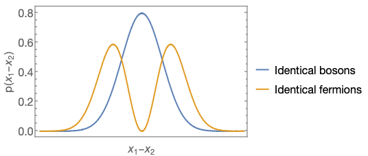
We can see that the two-electron wavefunction is zero when x_1 = x_2 due to the antisymmetry, and overall the effect of fermion statistics is that the two electrons repel each other, as opposed to the bosonic (symmetrized) case also shown where they are perfectly happy to coexist at the same point in space.
If we consider identical bosons instead of fermions, then symmetrizing does not result in any change to the energy spectrum, since the ground state is still n_1 = n_2 = 0. However, it does change the number of states available at each energy level. As an example, for a distinguishable pair of particles in an SHO, \ket{n_1 = 0, n_2 = 1} and \ket{n_1 = 1, n_2 = 0} are different states with the same energy. But for identical bosons, only the symmetrized combination of these two states is physical, so there is only one state instead of two with this energy. This is most significant in stat mech applications, which we’ll turn to now.
In the example above, we completely neglected the spin of the electrons for simplicity. Of course, real electrons do have spin, and it does matter since a spin-up electron is distinguishable from a spin-down electron. As you remember from chemistry class, an electronic state is only “filled” by a pair of electrons, one with each spin. If there are no other interactions, then two electrons in a SHO will still have the ground state \ket{n_1 = 0, n_2 = 0}, but they must have opposite spin orientations in this state.
This doesn’t mean that our example which ignored the spin is totally unrealistic. Since we’re considering a one-dimensional SHO, we can simply apply a strong magnetic field in a transverse direction to force the electron spins to be oriented the same way, at which point we’ll find the results for the energy spectrum as if we ignored the spin.
18.3 Diatomic molecules
Diatomic molecules give another classic example of the effects of identical particle statistics. As we’ve discussed before, the energy levels of a diatomic molecule are set by different ways in which the molecule can move: rotation, vibration, and internal excitations of the atoms themselves. The lowest-energy modes for a diatomic molecule are the rotational modes. If we’re interested only in these modes, we can study them by way of the rigid rotor Hamiltonian, \hat{H} = \frac{\hat{L}^2}{2I}, where \hat{\vec{L}} is the angular momentum of the molecule, and the moment of inertia I is determined entirely by the nuclei, so I = \mu a^2 with \mu the reduced mass and a the inter-nuclear distance. This is a very simple Hamiltonian to deal with: its energy eigenvalues are simply E_l = \frac{\hbar^2}{2I} l(l+1). If we have a heterogeneous molecule like OH, then all of these energy levels are present; the nuclear spin, in particular, is irrelevant since the distance between the two nuclei leads to a very small coupling.
However, for molecules composed of identical compounds, the situation is more complicated. Keep in mind that the nuclei set the properties of the quantum rotor spectrum, so we will be interested in the total wavefunction of the two nuclei here. For the hydrogen molecule H_2, each nucleus is a single proton, which is spin-1/2 and therefore a fermion. This time, we won’t ignore the protons’ spin: letting the label i=1,2 index over the two protons, proton i is at position \vec{x}_i and is in a spin state labelled by \hat{S}_{z,i} = \pm \tfrac{1}{2}. We’ll label the combined spin state in the usual shorthand, e.g. \ket{s_{z,1} = +\tfrac{1}{2}} \ket{s_{z,2} = -\tfrac{1}{2}} is written as \ket{\uparrow \downarrow}. Due to Fermi statistics, the overall state vector \ket{\psi} has to be anti-symmetric under \hat{P}_{12}. This gives us two options:
- The spin state is symmetric, for which there are three options: \ket{\uparrow \uparrow}, \ket{\downarrow \downarrow}, \frac{1}{\sqrt{2}} (\ket{\uparrow \downarrow} + \ket{\downarrow \uparrow}). These are the three possible S=1 (spin triplet) states in the addition of angular momentum problem for \mathbf{\tfrac{1}{2}} \otimes \mathbf{\tfrac{1}{2}}. In this case, the spatial wavefunction must be antisymmetric when we exchange \vec{x}_1 \leftrightarrow \vec{x}_2.
- The spin state is antisymmetric, for which there is only the S=0 (spin singlet) combination \frac{1}{\sqrt{2}} (\ket{\uparrow \downarrow} - \ket{\downarrow \uparrow}). For this spin state, the spatial wavefunction must be symmetric instead to give us overall anti-symmetry under \hat{P}_{12}.
The spin-symmetric triplet states are collectively known as ortho-H_2, while the antisymmetric singlet state is called para-H_2. How do we relate these symmetries to the allowed energy levels of the quantum rotor? In the particular case of a diatomic molecule, we notice that the permutation operator \hat{P}_{12} is also the parity operator! Therefore, all of the angular momentum eigenstates of the system, which in space correspond to spherical harmonics Y_l^m(\theta, \phi), are permutation eigenstates with eigenvalue (-1)^l. Thus, from our constraints on the symmetry of the spatial wavefunction, we see that ortho-H_2 states have only odd l, while for para-H_2 only even l are allowed.
Let’s see what this implies by doing a little statistical mechanics again. Defining the “rotational temperature” \Theta \equiv \frac{\hbar^2}{2Ik_B}, the general form of the partition function for a quantum rotor is Z_{\rm rot} = \sum_l N_l e^{-\beta E_l} = \sum_l (2l+1) e^{-l(l+1) \Theta / T}. However, as we have just argued for H_2, the ortho and para states will have different allowed values, and thus the sums will be different. In addition to knocking out some values of l, the ortho states pick up a factor of 3 since they have 3 allowed spin states per l value. Thus, we have the two partition functions Z_{o} = 3 \sum_{l=1,3,5...} (2l+1) e^{-l(l+1) \Theta / T}, \\ Z_{p} = \sum_{l=0,2,4...} (2l+1) e^{-l(l+1) \Theta / T}. In the high-temperature limit, the exponential becomes 1 and the difference between Z_o and Z_p becomes irrelevant, except for the counting factor of 3 (so \lim_{T \rightarrow \infty} Z_o / Z_p = 3, which reflects the fact that at high temperatures we expect there to be three times are much ortho-H_2 as para-H_2 in a sample of hydrogen gas.) From the partition function, the overall rotational energy stored in a given species is given by \left\langle E \right\rangle_s = -\frac{\partial}{\partial \beta} \ln Z_s, and then to get something more easily accessible in experiment, we take another derivative to get the molar heat capacity, C_{{\rm rot},s} = \frac{\partial \left\langle E \right\rangle_s}{\partial T}.
We can’t really evaluate this analytically very well, but a numerical evaluation leads to the following results:
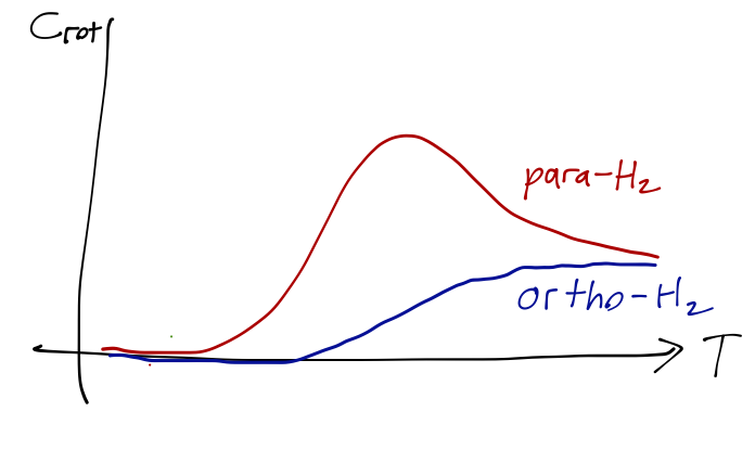
In a real H_2 gas at ordinary temperatures, the experimental curve lies somewhere in between these curves, corresponding to a roughly 3:1 mixture of ortho-H_2 to para-H_2; this is exactly the mixture we would predict from the degeneracy of the nuclear spin states. (In fact, this persists to fairly low temperatures even though the thermal equilibrium distribution when the temperature is low enough would be purely para-H_2; the spontaneous decay of ortho-H_2 to para-H_2 turns out to be a very slow process, which can be a nuisance if you want to liquify hydrogen and don’t want it to spontaneously boil itself away!)
Finally, the case where the two nuclei are bosonic, e.g. O_2, has the most dramatic effect. Each oxygen nucleus has 8 protons and 8 neutrons, each with spin-1/2; the overall total spin of the most common isotope, {}^{16}O, is s=0. Exchange symmetry for bosons thus requires that only symmetric states are allowed, and without any spin quantum numbers, the result is that all of the odd-l states (which are odd under parity) are completely removed from the rotational spectrum of molecular oxygen!
These missing states actually provided some early hint for the existence of the neutron, although the real historical story is more complicated since the most common isotope of nitrogen has spin s=1. This means that odd-l states aren’t completely forbidden, if they are paired with an antisymmetric spin state. But nevertheless, the emission spectrum for bosonic N_2 is very different from what we would predict if we didn’t know about the neutron, and assumed the nitrogen nucleus 7 protons was a fermion with half-integer spin. The experimental evidence to the contrary showed there must be some other physics at work!
18.4 Systems of multiple identical particles
Often in realistic systems, we’re dealing with many particles that are all identical instead of just pairs. Fortunately, it is straightforward to generalize what we’ve done so far to handle this case. If we have three identical particles 1,2,3, then we can define a set of permutation operators that swap pairwise labels: \hat{P}_{12}, \hat{P}_{13}, \hat{P}_{23}. Bosonic wavefunctions must be totally symmetric under the action of any of the permutation operators; fermionic wavefunctions are totally antisymmetric. In general, \hat{P}_{ij} \ket{\psi}_{\textrm{bosons}} = + \ket{\psi}_{\textrm{bosons}}, \\ \hat{P}_{ij} \ket{\psi}_{\textrm{fermions}} = - \ket{\psi}_{\textrm{fermions}}. For the three-particle case, we can construct the appropriately (anti-)symmetrized wavefunctions by inspection: \psi^S(1,2,3) = \frac{1}{\sqrt{6}} [\psi(1,2,3) + \psi(2,3,1) + \psi(3,1,2) \\ + \psi(1,3,2) + \psi(2,1,3) + \psi(3,2,1) ]. \\ \psi^A(1,2,3) = \frac{1}{\sqrt{6}} [\psi(1,2,3) + \psi(2,3,1) + \psi(3,1,2) \\ - \psi(1,3,2) - \psi(2,1,3) - \psi(3,2,1) ]. \\ The terms with minus signs in the fermionic wavefunction correspond to odd permutations, that is to say, permutations of \psi(1,2,3) generated by applying an odd number of pairwise permutation operators.
A useful shorthand for keeping track of the minus signs when we have a lot of fermions in a system is to use the Slater determinant. Given a set of one-particle fermion wavefunctions \ket{\chi}_1(p), ..., \ket{\chi}_N(p), where p labels which particle we apply the wavefunction to, the combined and totally antisymmetrized wavefunction is given by \psi^A(1,2,3,...,N) = \frac{1}{\sqrt{N!}} \left| \begin{array}{ccc} \chi_1(1) & \chi_1(2) & ... \\ \chi_2(1) & \chi_2(2) & ... \\ ... & ... & ... \end{array} \right|. The symmetry properties of the determinant match the required symmetry under permutation for a totally antisymmetric wavefunction. As an aside, we can use the Slater determinant to write down a bosonic wavefunction quickly too; we just ignore all the minus signs.
Construct the Slater determinant for three identical fermions in distinct one-particle states \psi_1(p), \psi_2(p), \psi_3(p), where p labels the particle. Show that swapping any two particles changes the sign of the determinant, demonstrating the antisymmetry of the wavefunction under particle exchange.
Answer:
The Slater determinant for three fermions is: \psi^A(1,2,3) = \frac{1}{\sqrt{6}} \left| \begin{array}{ccc} \psi_1(1) & \psi_1(2) & \psi_1(3) \\ \psi_2(1) & \psi_2(2) & \psi_2(3) \\ \psi_3(1) & \psi_3(2) & \psi_3(3) \end{array} \right|.
To demonstrate antisymmetry, swap particles 1 and 2. This corresponds to swapping the first and second columns of the determinant. A column swap changes the sign of a determinant, so: \psi^A(2,1,3) = \frac{1}{\sqrt{6}} \left| \begin{array}{ccc} \psi_1(2) & \psi_1(1) & \psi_1(3) \\ \psi_2(2) & \psi_2(1) & \psi_2(3) \\ \psi_3(2) & \psi_3(1) & \psi_3(3) \end{array} \right| = -\psi^A(1,2,3).
The Slater determinant is most often used for wavefunctions, but applies to any antisymmetric combination of states. For example, in the two-state example just above, we can write the antisymmetric state as a Slater determinant, \frac{1}{\sqrt{2}} (\ket{a}_1 \ket{a'}_2 - \ket{a'}_1 \ket{a}_2) = \frac{1}{\sqrt{2}} \left| \begin{array}{cc} \ket{a}_1 & \ket{a}_2 \\ \ket{a'}_1 & \ket{a'}_2 \end{array} \right|.
As a comment in passing, when we have multiple particles involved at once, the symmetry group expands to the permutation group S_n for n particles. Bosonic wavefunctions inhabit the trivial representation of S_n, meaning that any permutation just gives +1 back, corresponding to total symmetry. Fermionic wavefunctions exist in the sign representation, which maps odd numbers of permutations to -1 instead of +1. Other representations of S_n exist, but because of spin-statistics, only these two simple representations are allowed in quantum mechanics.
18.4.1 Fermi energy and degeneracy pressure
The general case of a large number of non-interacting fermions is interesting and important (serving as a starting unperturbed system for many condensed-matter applications, for example.) If we have N such fermions and their one-particle energy eigenstates are given by \hat{H}_i u_{E_k}(i) = E_k u_{E_k}(i) where \hat{H} = \sum_{i=1}^N \hat{H}_i is just a sum of N identical non-interacting Hamiltonians, then any combined energy eigenstate can be written as a product of u_{E_k}(i). To keep track of all the signs in forming the antisymmetrized wavefunction, we use the Slater determinant as written above, u^A(1,2,3,...,N) = \frac{1}{\sqrt{N!}} \left| \begin{array}{ccc} u_{E_1}(1) & u_{E_1}(2) & ... \\ u_{E_2}(1) & u_{E_2}(2) & ... \\ ... & ... & ... \end{array} \right|. An immediate consequence of the anti-symmetry that we can read off from the determinant is that to be able to write a wavefunction at all for a system of N fermions, there must be at least N distinct states for the fermions to exist in. Up to degeneracy, this means in particular that accommodating N fermions at once requires filling up all available states up to a certain energy level, known as the Fermi energy (as we saw in the simple two-electron example above.)
I won’t go through a detailed calculation of the Fermi energy; you can find some detail in Sakurai, or in any stat mech book. Besides, the value of the Fermi energy is given by a sum over energy states, and depends on what system we’re trying to study. But I do want to stress that the Fermi energy is inherently different from a zero-point energy shift; it really does have physical consequences. Let’s look at one particular example, which is a white dwarf star.
White dwarves are stars which have burned off all of their fuel; nuclear fusion stops, and the pressure that the fusion provides against gravitational collapse ceases. As a result, the star becomes very dense. (The full astrophysical story here is more complicated than this, but we’re interested in the end result right now.) The gravitational binding energy of the white dwarf is given by a simple classical calculation, E_G = -\frac{3}{5} \frac{GM^2}{R} The change in energy with respect to volume gives a corresponding pressure, P_G = \partial E_G / \partial V. However, there is another effect at work here; the squeezed matter which makes up the white dwarf exists as electron-degenerate matter, in which the electrons are stripped away from the nuclei and essentially exist as an electron gas. If we have an electron gas confined to a fixed volume, then the energy levels available are restricted by the wave number k = 2\pi / L. A straightforward calculation gives the result E_e = \frac{3\hbar^2}{10m_e} N_e \left(\frac{3\pi^2 N_e}{V}\right)^{2/3}. for a gas of N_e electrons in volume V.
It’s more stat mech than quantum mechanics, but I’ll put a quick Fermi energy derivation here nevertheless, since it does rely on what we’ve developed about identical particles.
Our model will be the three-dimensional particle in a box: assume a zero potential for 0 \leq x, y, z \leq L and infinite potential outside. There’s no need to use our machinery for rotations in three dimensions, since this system just decouples into three one-dimensional particle-in-a-box systems. The wavefunction is the product of one-dimensional solutions \psi_{n_x,n_y,n_z}(x,y,z) = \sqrt{\frac{8}{L^3}} \sin \left( \frac{n_x \pi x}{L} \right) \sin \left( \frac{n_y \pi y}{L} \right) \sin \left( \frac{n_z \pi z}{L} \right), and the energy is the sum E_{n_x,n_y,n_z} = \frac{\pi^2 \hbar^2}{2mL^2} (n_x^2 + n_y^2 + n_z^2).
Now, we suppose that the box is filled with N_e electrons, where N_e is very large. Neglecting interactions between the electrons, the key effect is that each energy level \ket{n_x, n_y, n_z} can only support 2 electrons; one with spin up, and one with spin down. The total energy is then just the sum, E_{\rm tot} = \sum_{n_x,n_y,n_z} 2E_{n_x,n_y,n_z} = \frac{\pi^2 \hbar^2}{mL^2} \sum_{n_x,n_y,n_z} (n_x^2 + n_y^2 + n_z^2). By assumption, N_e is very large, which means we can replace the sum with an integral, E_{\rm tot} \approx \frac{\pi^2 \hbar^2}{m_eL^2} \int dn_x dn_y dn_z (n_x^2 + n_y^2 + n_z^2) \\ = \frac{\pi^2 \hbar^2}{m_eL^2} \frac{\pi}{2} \int_0^{n_{\rm max}} dn\ n^4, \\ = \frac{\pi^3 \hbar^2}{10m_eL^2} n_{\rm max}^5, switching to spherical coordinates and doing the angular integral - it only runs over the first octant since all of the n_x,n_y,n_z must be positive, so we get 4\pi/8 from the solid angle.
Now we just need to know what n_{\rm max} is. We can write this as an integral as well, since it’s just 2 for each state, so N_e = \sum_{n_x,n_y,n_z} 2 = 2 \frac{\pi}{2} \int_0^{n_{\rm max}} dn\ n^2 \\ = \frac{\pi}{3} n_{\rm max}^3, or n_{\rm max} = (3 N_e / \pi)^{1/3}. Plugging back in, E_{\rm tot} = \frac{\pi^3 \hbar^2}{10m_eL^2} (3 N_e/\pi)^{5/3} \\ = \frac{3\hbar^2}{10m_e} N_e \left(\frac{3\pi^2 N_e}{V}\right)^{2/3}. Now, this is not the Fermi energy; the Fermi energy is the level of the highest filled energy level. Appealing to some textbook stat mech that I won’t reproduce here, the total energy is related to the Fermi energy as E_{\rm tot} = \frac{3}{5} N_e E_F from which we read off E_F = \frac{\hbar^2}{2m_e} \left( \frac{3 \pi^2 N_e}{V}\right)^{2/3}, matching the textbook result.
The derivative \partial E_F / \partial V once again gives a pressure, which is known as the degeneracy pressure. This opposes the gravitational pressure, and in fact if we rewrite the gravitational energy as E_G = -\frac{3}{5} G (N_n M_n)^2 \left( \frac{4\pi}{3} \right)^{1/3} V^{-1/3} and then calculate the pressures and balance them, we can predict that the radius of a white dwarf should be approximately 7,000 km (see here for some details.) So a white dwarf packs an entire solar mass into a space the size of the Earth - very compact!
If a white dwarf can go on to acquire more mass (by accreting from a partner star, say), then eventually the available Fermi energy increases to the point that the electrons are fused into the protons, leaving neutrons (and neutrinos) - this gives a supernova (type Ia), and leaves behind a neutron star, which is once again supported by degeneracy pressure. The stellar radius in our degeneracy pressure estimate scales inversely with the mass m of the fermion, so the predicted size of a neutron star would be 7000\ {\rm km} \times (m_e / m_n) \sim 4\ {\rm km}; we shouldn’t take this number too seriously since neutrons are strongly interacting, but real neutron stars have observed radii on the order of 10 km, so it’s not too far off.