30 Time-dependent perturbation theory
Now that we have a few more tricks to deal with time dependence, let’s turn to the more general approach of perturbation theory. We will tackle the general case where a time-independent Hamiltonian \hat{H}_0 is perturbed by a time-dependent term, \hat{H} = \hat{H}_0 + \hat{V}(t). This may seem insufficiently general, but as with time-independent perturbation theory, the idea here will be to use the exact solution to \hat{H}_0 as a foundation to expand around. As this is a perturbative approach we assume \hat{V} \ll \hat{H}_0 in some sense (I won’t use an explicit small parameter \lambda here, since it will be clearer how the perturbation appears once we start calculating.) We typically also assume that \hat{V}(t) is transient, meaning that as t \rightarrow \pm \infty it goes to zero, so that we can describe initial and final states of the system purely in terms of \hat{H}_0.
Formally, it is important that the perturbation doesn’t exist at t \rightarrow \pm \infty; since \hat{H}_0 is the only thing we can solve, in order to describe the initial and final states completely we need them to be purely expanded in \hat{H}_0 eigenstates.
In some situations, the perturbation we will deal with is explicitly switched on and off, so that it satisfies the condition. However, we will be considering some important examples of time-dependent perturbations that don’t vanish at large times, for example a harmonic perturbation of the form V_0 \cos(\omega t). In this case, you should imagine that the perturbation is turned on and off adiabatically at very large times, for example by applying a very slow exponential damping \exp(-\epsilon|t|). You can do this explicitly and take \epsilon \rightarrow 0 carefully for cases where the details seem potentially important.
30.1 Derivation of time-dependent perturbation theory
Given this setup, the path integral provides us with a beautiful and clear way to derive the formulas describing perturbation in \hat{V}(t). Recall that the path integral allows us to compute the transition amplitude between two states \left\langle x_f, t_f | x_i, t_i \right\rangle by writing a formal sum over all possible paths from one space-time point to the other (which becomes an integral when the available paths are continuous and infinite.)
For present purposes, instead of expanding in position eigenstates, let’s expand in the energy eigenstates \{ n \} of \hat{H}_0. Specifically, we will compute the matrix elements of the time evolution operator \hat{U}(t, t_0) over these states, U_{fi}(t_f, t_i) = \bra{f} \hat{U}(t_f, t_i) \ket{i}. This quantity is known as the transition amplitude from initial state i at time t_i to final state f at time t_f (again, both are \hat{H}_0 eigenstates.) The time evolution operator is difficult to write down in general, but if we suppose that the time elapsed t_f - t_i is very small, then we can write the approximate form \hat{U}(t_f, t_i) \approx \exp \left( \frac{-i (\hat{H}_0 + \hat{V}(t_i)) (t_f-t_i)}{\hbar} \right). (Note that we’re ignoring the evolution of \hat{V}(t) itself between t_i and t_f; this is justified, for example, if t_f - t_i is very small, and we’ll worry more about this expansion below.) Squaring the transition amplitude gives us the transition probability, p_{i \rightarrow f}(t_f) = |U_{fi}(t_f, t_i)|^2, and if we have the entire matrix U_{fi}(t_f, t_i), then we can time-evolve any initial state \ket{\psi(t_i)} \rightarrow \ket{\psi(t_f)} by expanding it in energy eigenstates and then applying the matrix. If we only had \hat{H}_0, of course, then U_{fi}(t_f, t_i) \propto \delta_{fi}, and the transition probability to any other state is zero. It is only the presence of a perturbation \hat{V}(t) that will allow transitions between different energy eigenstates.
Now, we’d like to proceed by expanding the evolution operator in the limit that \hat{V} is small. Since \hat{H}_0 and \hat{V}(t) are operators and in general don’t commute, we have to proceed carefully. We’ll make use of the Zassenhaus formula, which is another corollary of the previously-seen Baker-Campbell-Hausdorff formula: e^{t(\hat{A} + \hat{B})} = e^{t\hat{A}} e^{t\hat{B}} e^{-\frac{t^2}{2} [\hat{A}, \hat{B}]} \left(1 + \mathcal{O}(t^3) \right), where there are an infinite number of terms of order t^3 and higher, each of which contains an increasing number of commutators between the operators \hat{A} and \hat{B}.
This will allow us to proceed and expand in small \hat{V}(t), but we see that to do so we need the time elapsed in the exponential to be small. If we let t = t_i + \Delta t, then from above, \hat{U}(t_i + \Delta t, t_i) \approx e^{-i \hat{H}_0 (\Delta t)/\hbar} \left( 1 - \frac{i\hat{V}(t_i) (\Delta t)}{\hbar} + \mathcal{O}((\Delta t)^2) \right), where the neglected terms are, explicitly, -\frac{\hat{V}(t_i)^2 (\Delta t)^2}{2\hbar^2} + \frac{[\hat{H}_0, \hat{V}] (\Delta t)^2}{2\hbar^2} + \mathcal{O}((\Delta t)^3). So, schematically, the conditions we need for our perturbation expansion to be valid (i.e. to just keep the first \hat{V}-dependent term, which is what we will do) are \hat{V}(t_i) \ll \frac{\hbar}{\Delta t},\ \ [\hat{H}_0, \hat{V}(t_i)] \ll \frac{\hbar^2}{(\Delta t)^2}. In normal circumstances, as long as there is a sufficiently small parameter in front of \hat{V}, both of these conditions will be satisfied.
Of course, we don’t want to be restricted to only studying time evolution over infinitesimal amounts of time. To get around that, we come back to the idea of path integration. We can compose two evolution operators if we insert a complete set of states: U_{fi}(t_f, t_i) = \bra{f} \hat{U}(t_f,t_i) \ket{i} \\ = \sum_{n_1} \bra{f} \hat{U}(t_f, t_1) \ket{n_1} \bra{n_1} \hat{U}(t_1, t_i) \ket{i} \\ = \sum_{n_1} U_{fn_1}(t_f, t_1) U_{n_1i}(t_1, t_i) splitting the time evolution up as well. Now we break the time evolution into N steps of duration \Delta t: U_{fi}(t_f, t_i) = \sum_{n_1} \sum_{n_2} ... \sum_{n_N} U_{fn_1}(t, t_1) U_{n_1n_2}(t_1, t_2) ...U_{n_Ni}(t_N, t_i) \\ = \sum_{n_1} \sum_{n_2} ... \sum_{n_N} \bra{f} e^{-i\hat{H} \Delta t/\hbar} \ket{n_1} \bra{n_1} e^{-i\hat{H} \Delta t/\hbar} \ket{n_2} \bra{n_2}... \ket{n_N} \bra{n_N} e^{-i \hat{H} \Delta t/\hbar} \ket{i} So far, this is still exact, but now we can plug in our series expansion from above. As long as N is large enough, then \Delta t will be small enough for it to be valid. However, if we keep the order-\hat{V} term in each insertion, then the overall expression has terms up to order \hat{V}^N. Instead, as we did for time-independent perturbation theory, we should organize corrections by order in the expansion, U_{fi}(t_f, t_i) \approx U_{fi}^{(0)}(t_f, t_i) + U_{fi}^{(1)}(t_f, t_i) + U_{fi}^{(2)}(t_f, t_i) + ... where U_{fi}^{(n)}(t_f, t_i) contains the perturbation \hat{V}(t) exactly n times.
Now we can start writing these terms out explicitly. The zeroth-order term has no \hat{V}(t) at all, U_{fi}^{(0)}(t_f, t_i) = \sum_{n_1} \sum_{n_2} ... \sum_{n_N} \bra{f} e^{-i\hat{H}_0 \Delta t/\hbar} \ket{n_1} ...\bra{n_N} e^{-i\hat{H}_0 \Delta t/\hbar} \ket{i} \\ = \bra{f} e^{-iE_i (t_f-t_i)/\hbar} \ket{i} = \delta_{fi} e^{-iE_i (t_f-t_i)/\hbar}, recollapsing the sum and using the fact that these are all eigenstates of \hat{H}_0.
At first order, we have all possible terms with a single insertion of \hat{V} somewhere. Let’s write it out by adding one more sum to keep track of which matrix element we put it next to: U_{fi}^{(1)}(t_f, t_i) = \sum_k V_{fi}^{(k)}(t_f, t_i) \\ V_{fi}^{(k)}(t_f, t_i) = \sum_{n_1} \sum_{n_2} ... \sum_{n_N} \bra{f} e^{-i\hat{H}_0 \Delta t/\hbar} \ket{n_1} ... \bra{n_{k-1}} e^{-i\hat{H}_0 \Delta t/\hbar} \left( - \frac{i\hat{V}(t_k) (\Delta t)}{\hbar} \right) \ket{n_k} ... As with the zeroth-order term, any sequence of matrix elements that only contain \hat{H}_0 can all be collapsed together, since they can only connect the same energy eigenstate to itself. So we can collapse all of the sums down: V_{fi}^{(k)}(t_f, t_i) = -e^{-iE_{f}(t_f-t_k)/\hbar} \bra{f} \frac{i\hat{V}(t_k) \Delta t}{\hbar} \ket{i} e^{-iE_i(t_k-t_i)/\hbar} where we acted to the left with e^{-i\hat{H}_0 \Delta t/\hbar}. The only remaining dependence on the index k denoting where the perturbation has been inserted is in the appearance of the time t_k. In terms of our “path integral”, the physical statement here is that since only \hat{V} can allow us to change energy levels, the sum over all possible paths has collapsed to the paths where we are in either state \ket{i} or \ket{f}, switching at the moment the perturbation happens.
To complete the analogy to path integration, there is no reason to keep the time interval \Delta t finite, since it was an arbitrary choice we made when subdividing the “paths”. Plugging back in and taking the limit converts the remaining sum to an integral, and we find: U_{fi}^{(1)}(t_f, t_i) = \lim_{N \rightarrow \infty} \sum_k -e^{-iE_f(t_f-t_k)/\hbar} \bra{f} \frac{i\hat{V}(t_k) \Delta t}{\hbar} \ket{i} e^{-iE_i(t_k-t_i)/\hbar} \\ = -\frac{i}{\hbar} \int_{t_i}^{t_f} dt e^{-iE_f(t_f-t)/\hbar} \bra{f} \hat{V}(t) \ket{i} e^{-iE_i(t-t_i)/\hbar}.
Physically, it’s easy to read off what is happening: the system evolves by the usual phase in eigenstate \ket{i} until time t, at which point the perturbation acts and the system transitions into \ket{f}. From that point forwards, the system propagates in state \ket{f} until the final time t_f. Since the perturbation only happens once but can happen at any moment in the interval, we integrate over all possible times t at which it occurs.
We will almost exclusively work with this first-order formula, but since we have gone through the formalism, it’s worth briefly discussing what the higher-order corrections look like. Going back to our (note: not in interaction picture) insertion-of-states expression from above, U_{fi}(t_f, t_i) = \sum_{n_1} \sum_{n_2} ... \sum_{n_N} \bra{f} e^{-i\hat{H} \Delta t/\hbar} \ket{n_1} \bra{n_1} e^{-i\hat{H} \Delta t/\hbar} \ket{n_2} \bra{n_2}... \ket{n_N} \bra{n_N} e^{-i \hat{H} \Delta t/\hbar} \ket{i}, the second-order term U_{fi}^{(2)} will consist of all possible insertions of two copies of \hat{V} at two different times. (Inserting twice in the same timeblock, which is the correction we ignored by expanding e^{-i\hat{H} \Delta t/\hbar} only to first order, is suppressed and vanishes as the number of segments N \rightarrow \infty.) If we go through the same arguments as above, this will leave us with the result U_{fi}^{(2)} = \left(-\frac{i}{\hbar}\right)^2 \sum_n \int_{t_i}^{t_f} dt_2 \int_{t_i}^{t_2} dt_1 e^{-iE_f(t_f-t_2)/\hbar} \bra{f} \hat{V}(t_2) \ket{n} e^{-iE_n(t_2-t_1)/\hbar} \bra{n} \hat{V}(t_1) \ket{i} e^{-iE_i(t_1-t_i)/\hbar}. Note that to avoid double-counting, the integral limits and variables are defined to enforce time-ordering, so that the events always happen in the same order in time: we transition from \ket{i} \rightarrow \ket{n} \rightarrow \ket{f}, and t_2 is always the time associated with the latter transition. Again, this is easy to interpret physically: we’re stuck with a sum over intermediate states \ket{n} this time, since we can transition to any other energy eigenstate in the middle before going to \ket{f} if we have two insertions of \hat{V}.
You can see the pattern here, that each order just involves an extra insertion of time-ordered factors of \hat{V}(t), with complete sets of states inserted as needed but with the initial and final states held fixed. We can write down a diagrammatic sketch that encapsulates this idea:
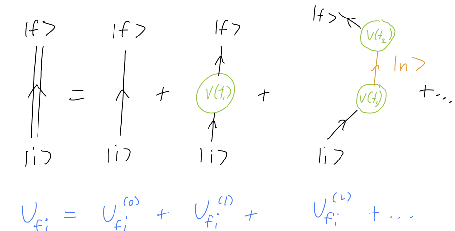
This is sort of a generic picture, making no assumptions about \ket{i} or \ket{f}. If we think about the specific case where \ket{f} \neq \ket{i} and try to delineate states using horizontal position, with the perturbation matrix \hat{V} acting as a “box” that can mix them together, we can draw a similar set of diagrams with a little more structure:
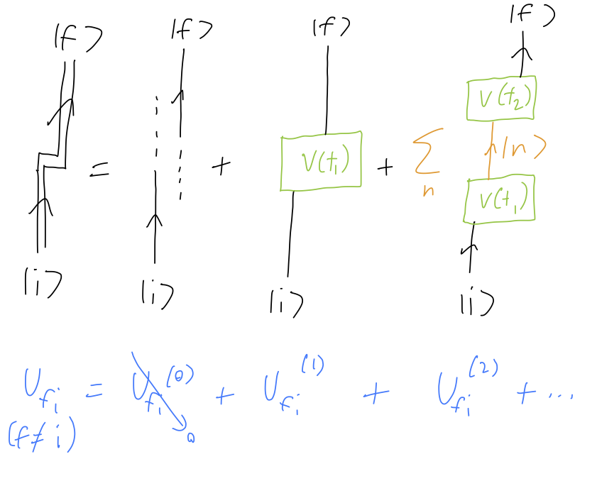
Here, the diagrams may help give us a better mental picture of what’s happening: but in more detailed calculations, particularly in quantum field theory or in many-body physics (where the analogous diagrams are known as Feynman diagrams), the diagrammatic expansion is actually a very important calculational tool. The diagrammatic approach is standard in any quantum field theory textbook; if you are interested an introduction to this approach from a many-body point of view, I recommend Mattuck’s book on Feynman diagrams.
30.1.1 Going to interaction picture
Everything we’re doing here can be much more compactly expressed if we switch to interaction picture (see Section 7.4 if you need a reminder). Briefly, this means that we allow our operators to obey a Heisenberg equation using just \hat{H}_0, which means that the interaction-picture version of \hat{V}(t) is (evolving from time t=0) \hat{V}^{(I)}(t) = e^{i\hat{H}_0 t/\hbar} \hat{V}(t) e^{-i\hat{H}_0 t/\hbar}. In the matrix element \bra{f} \hat{V}(t) \ket{i}, the extra factors which are introduced here kick out precisely the phases that we’re looking for. Since the states evolve according to just the perturbation \hat{V} in interaction picture, the time-evolution operator \hat{U}(t_f, t_i) itself picks up the same factors but conjugated, to cancel the \hat{H}_0 part of the evolution: \hat{U}^{(I)}(t_f, t_i) = e^{-i\hat{H}_0 t_f/\hbar} \hat{U}(t_f, t_i) e^{i\hat{H}_0 t_i/\hbar}. Computing transition matrix elements of the interaction-picture operator \bra{f} \hat{U}_I(t_f, t_i) \ket{i}, we therefore find an extra factor of e^{-iE_f t_f/\hbar} e^{+iE_i t_i/\hbar}, which matches the two factors from above that don’t depend on t. Thus, in interaction picture we find the much more compact result: U^{(I,1)}_{fi} = -\frac{i}{\hbar} \int_{t_i}^{t_f} dt \bra{f} \hat{V}^{(I)}(t) \ket{i} (you can verify by plugging back in that this gives back the result we had above.)
Given a Hamiltonian of the form \hat{H}_0 + \hat{V}(t) with \hat{V}(t) small compared to \hat{H}_0, and working in interaction picture, to first order in perturbation theory the transition matrix element from initial state \ket{i} at time t_i to final state \ket{f} and time t_f is U^{(I)}_{fi} \approx \delta_{fi} - \frac{i}{\hbar} \int_{t_i}^{t_f} dt \bra{f} \hat{V}^{(I)}(t) \ket{i}. or in the Schrödinger picture, U_{fi} \approx \delta_{fi} - \frac{i}{\hbar} \int_{t_i}^{t_f} dt\ e^{-iE_f (t_f-t)/\hbar} \bra{f} \hat{V}(t) \ket{i} e^{-iE_i(t-t_i)/\hbar}.
Interaction picture also makes it much more compact to write out the higher-order terms:
Given a time-dependent perturbation theory problem \hat{H}_0 + \hat{V}(t) set up in interaction picture, the full perturbative series solution for the time evolution operator can be written as \hat{U}^{(I)}(t_f, t_i) = \hat{1} - \frac{i}{\hbar} \int_{t_i}^{t_f} dt_1 \hat{V}^{(I)}(t_1) + \left( -\frac{i}{\hbar} \right)^2 \int_{t_i}^{t_f} dt_2 \int_{t_i}^{t_2} dt_1 \hat{V}^{(I)}(t_2) \hat{V}^{(I)}(t_1) \\ + \left( -\frac{i}{\hbar} \right)^3 \int_{t_i}^{t_f} dt_3 \int_{t_i}^{t_3} dt_2 \int_{t_i}^{t_2} dt_1 \hat{V}^{(I)}(t_3) \hat{V}^{(I)}(t_2) \hat{V}^{(I)}(t_1) + ... This is known as the Dyson series.
This is written at the level of operators, which makes it much more compact; if we want to find specific matrix elements, we’ll have to insert sums over intermediate states into each term to recover the expressions we wrote above.
As a warning when comparing to other references, I’ll stress that we now have formulas that allow us to find the full time dependence. In the general case, any arbitrary state can always be decomposed into energy eigenstates, which means at any time t we can write \ket{\psi(t)} = \sum_n c_n(t) \ket{n}. (Here I assume interaction picture for simplicity, which means there are phases lurking in the definitions of c_n(t) compared to the same expansion in Schrödinger picture!) Formally, the evolution is described by the time-evolution operator, which means that \ket{\psi(t)} = \hat{U}(t, t_0) \ket{\psi(t_0)}. Expanding in energy eigenstates, \sum_n c_n(t) \ket{n} = \sum_n \hat{U}(t,t_0) c_n(t_0) \ket{n} or selecting out a single matrix element by dotting in \bra{m}, c_m(t) = \sum_n U_{mn}(t,t_0) c_n(t_0). If we find the matrix in the middle directly, as we are currently doing, then we have solved the problem. However, some references will instead begin with the representation in terms of c_n(t) and write the interaction-picture Schrödinger equation instead; if you do so, you will find the result i\hbar \frac{d c_n}{dt} = \sum_m V_{nm}(t) c_m(t) in interaction picture, where the perturbation matrix element V_{nm} has appeared from differentiating the interaction-picture time evolution operator \hat{U}. Passing back to Schrödinger picture would introduce some extra E_m-dependent phases, so I won’t bother to do it explicitly. Here we will stick to the operator solution method that we’ve already found, but I wanted to make this connection for completeness.
30.2 Test solution: magnetic resonance
As we usually do in these notes, let’s start with an example problem in a system where we also have access to the exact solution. We’ll consider a two-state system with the Hamiltonian \hat{H} = \hbar \omega \hat{\sigma}_z + \hbar \epsilon(t) \hat{\sigma}_x = \left(\begin{array}{cc} \hbar \omega & \hbar\epsilon(t) \\ \hbar \epsilon(t) & -\hbar \omega \end{array} \right) with \epsilon(t) \ll \omega, so that the \hat{\sigma}_z term acts as our \hat{H}_0 and the \hat{\sigma}_x term is our perturbation. Let’s start with just a constant perturbation, \epsilon(t) = \epsilon; we’re still doing time-dependent PT as long as we’re studying time dependence and transitions, even if the perturbation is constant (in fact, this is an important case!) Our basis states provided by \hat{H}_0 are \{\ket{\uparrow}, \ket{\downarrow}\} with energy eigenvalues E_+ = +\hbar \omega, E_- = -\hbar \omega respectively.
Suppose our initial state at time t=0 is \ket{\uparrow}, and we want to consider the transition to \ket{\downarrow}. Then we have U^{(I)}_{\downarrow \uparrow}(t) \approx - \frac{i}{\hbar} \int_0^t dt' \bra{\downarrow} \hat{V}^{(I)}(t') \ket{\uparrow}. Interaction picture was convenient for writing these compactly, but let’s go back to Schrödinger picture by reintroducing the energy phases since that’s the solution we’ll be matching back on to. We have U_{\downarrow \uparrow}(t) \approx -\frac{i}{\hbar} \int_0^t dt' e^{-iE_\downarrow(t-t')/\hbar} \bra{\downarrow} \hat{V} \ket{\uparrow} e^{-iE_\uparrow t'/\hbar} \\ = \frac{-i}{\hbar} e^{i\omega t} \int_0^t dt' e^{-2i\omega t'} (\hbar \epsilon) \\ = \frac{\epsilon}{2\omega} e^{i\omega t} \left[ e^{-2i\omega t} - 1 \right] = -\frac{i\epsilon}{\omega} \sin (\omega t), giving a transition probability p_{\downarrow}(t) \approx \frac{\epsilon^2}{\omega^2} \sin^2 (\omega t).
Now we need the exact solution to compare to. With \epsilon(t) constant, this is exactly the Hamiltonian for magnetic resonance from Section 4.2 in the limit \nu \rightarrow 0, for which we found p_{\downarrow}(t) = \frac{\Omega_0^2}{\Omega^2} \sin^2 \left( \frac{\Omega t}{2} \right). Matching notation on to what we’re currently using and setting \nu=0, we have \Omega_0 \rightarrow 2\epsilon and \Omega \rightarrow 2\sqrt{\omega^2 + \epsilon^2}, so the exact solution is p_{\downarrow}(t) = \frac{\epsilon^2}{\epsilon^2 + \omega^2} \sin^2 \left( \sqrt{\omega^2 + \epsilon^2} t\right) \approx \frac{\epsilon^2}{\omega^2} \sin^2 (\omega t) carrying out a series expansion to order \epsilon^2; our result matches exactly.
In this example, you might be tempted to try to calculate the transition matrix element U_{\uparrow \uparrow}(t) as well for completeness. We can write out the expression for it at first order in perturbation theory easily enough: U^{(I)}_{\uparrow \uparrow}(t) \approx 1 - \frac{i}{\hbar} \int_{0}^t dt' \bra{\uparrow} \hat{V}^{(I)}(t') \ket{\uparrow}, However, since \hat{V} is proportional to \hat{\sigma}_x which is purely off-diagonal, the perturbation vanishes, so we see that U_{\uparrow \uparrow}(t) = 1 + \mathcal{O}(\epsilon^2). This might seem like a contradiction, since at any order in perturbation theory we should be able to conserve probability. But this seems to be telling us that p_{\uparrow \uparrow} = 1, which means there is no probability left for the transition to \ket{\downarrow} that we found!
The resolution to this apparent paradox is to notice that the transition probability p_\downarrow(t) is the square of the transition amplitude, so at first order it is proportional to \epsilon^2. This is generically true, except for the transition to the same state; since we have U_{\uparrow \uparrow} = 1 + (...) \epsilon^2, squaring it will give a transition probability of order \epsilon^2 only from the second-order term in the amplitude. Which is to say that if we want all our probabilities to be self-consistent, we need to go to higher order for the same-state transition.
Intuitively, the reason that we need to worry about second order for the amplitude to remain in the same state is that transitions of the form \ket{i} \rightarrow \ket{f} \rightarrow \ket{i} are important to consider. In a classical system, we normally wouldn’t worry about this sort of effect; the decay of a radium nucleus is an irreversible, one-way process. But in quantum mechanics, the evolution of our system is unitary and reversible, and we have to account for the process \ket{f} \rightarrow \ket{i} as well. We’ll worry more about this later, and for now just focus on specific transitions out of an initial state.
Of course, nobody wants to go to higher order in perturbation theory when it can be avoided! Since this issue applies uniquely to the same-state transition, if all we want is the probability to remain in state \ket{i}, we can just calculate all of the other transition probabilities and then impose normalization: p_{i \rightarrow i}(t) = 1 - \sum_{f \neq i} p_{i \rightarrow f}(t). There is more interesting physics lurking in the amplitude U_{ii}(t), but we’ll save that discussion for later.
Here, you should complete Tutorial 14 on “Time-dependent perturbation theory”. (Tutorials are not included with these lecture notes; if you’re in the class, you will find them on Canvas.)
30.3 Constant perturbation
Although we did it for the two-state system, the result we found above for first-order perturbative transitions with a constant perturbation is easy to generalize. Let’s consider the case where \hat{V}(t) is constant (which, again, you can think of as a potential which is adiabatically switched on and off rather than being truly constant, so that our initial and final states are properly eigenstates of \hat{H}_0.) To first order in perturbation theory, the general result is U_{fi}(t) = -\frac{i}{\hbar} \int_0^t dt' e^{-iE_f(t-t')/\hbar} \bra{f} \hat{V} \ket{i} e^{-iE_it'/\hbar}. Since the perturbation is constant, we can just pull it out of the integral, along with an overall phase: U_{fi}(t) = -\frac{i}{\hbar} V_{fi} e^{-iE_f t/\hbar} \int_0^t dt' e^{+i(E_f-E_i)t'/\hbar} \\ = -\frac{V_{fi}}{E_f-E_i} e^{-iE_f t/\hbar} \left[ e^{+i(E_f-E_i)t/\hbar} - 1 \right] \\ = -\frac{V_{fi}}{E_f-E_i} e^{-i(E_f+E_i)t/(2\hbar)} \left[ e^{+i\omega_{fi}t/2} - e^{-i\omega_{fi} t/2} \right] defining \omega_{fi} \equiv (E_f - E_i) / \hbar. Simplifying the difference of exponentials, we find U_{fi}(t) = \frac{-2i V_{fi}}{\hbar \omega_{fi}} e^{-i(E_f + E_i)t/(2\hbar)} \sin \left(\frac{\omega_{fi} t}{2} \right), and for the transition probability, p_{i \rightarrow f}(t) = |U_{fi}(t)|^2 = \frac{4|V_{fi}|^2}{\hbar^2 \omega_{fi}^2} \sin^2 \left( \frac{\omega_{fi} t}{2} \right). We see that transitions are allowed into any state for which V_{fi} is non-zero, with a timescale set by the energy difference between the states.
As a useful variation on this, we can use this in order to get the lifetime of our initial state i, meaning the probability it will stay in that state over time. As discussed above, rather than computing the probability for i \rightarrow i directly, this is best handled by computing the probability of transition to any other state and then subtracting. To get the latter, we just sum over final states: p_{i \rightarrow {\rm any}}(t) = \sum_{n \neq i} \frac{4|V_{ni}|^2}{(E_n - E_i)^2} \sin^2 \left( \frac{\omega_{ni} t}{2} \right). This formula is correct, but in general gives a complicated sum over lots of oscillating terms. To get to a more practical formula for the lifetime of a quantum state, we’re going to add some additional assumptions.
30.3.1 Density of states
The first key assumption will be that we’re in the situation where the number of available energy eigenstates \ket{n} is very large, which allows us to replace the sum with an integral and treat the n label as continuous, \sum_n \rightarrow \int dn. Since the energy of the states \ket{n} appears directly in our expression, it is more convenient to change variables to energy, \int dn = \int dE_n \rho(E_n), where the function \rho(E_n) is the density of states. Evidently, this is just the Jacobian dn/dE_n for our change of variables; physically, we should think of the density of states as counting the number of states available for a given energy value E_n.
As an instructive example, consider a particle of mass m in a cubic box of volume V = L^3 (so the potential is zero inside the box region and jumps to infinity outside.) The energy levels are given by E_{n_x, n_y, n_z} = \frac{\pi^2 \hbar^2}{2mL^2} (n_x^2 + n_y^2 + n_z^2) = \frac{\pi^2 \hbar^2}{2mL^2} \vec{n}^2.
In these notes, I’m studying a “real” box to compute the density of states. In other sources, you may see a calculation which instead uses a box of size L^3 with periodic boundary conditions. Periodic boundaries allow us to keep plane-wave solutions even in a finite box, as opposed to the hard boundaries I’m imposing here which would lead to sines that vanish at the box edges. Periodic boundaries also give slightly different results for the energy levels and other quantities by factors of 2.
In the limit that we’re studying where the discrete quantum states become continuous enough to replace sums with integrals, it turns out that the distinction in boundary conditions doesn’t matter for the density of states; either version gives the same answer. Physically, the density of states is set by behavior “inside the box” and the boundary effects become negligible. For further discussion, see chapter 4 of Merzbacher.
I’ll note in passing that the vector of integer energy-level labels \vec{n} is related to the wave vector \vec{k}; since E_n = \hbar^2 k^2 / (2m), we see that \vec{k} = \frac{\pi}{L} \vec{n}. Now we pass to the limit where the values of n are very large, so that \vec{n} becomes approximately continuous. Then we have \sum_{\vec{n}} \approx \int d^3n. To continue, we suppose that the sum is done over quantities that depend on the energy E_n, which means they only depend on \vec{n} through its magnitude n. This means that we switch to spherical coordinates and do the angular integrals, \int d^3n = \frac{\pi}{2} \int dn\ n^2 Note that this is a factor of 8 smaller than the usual solid angle, since all of the n_x, n_y, n_z components are restricted to be positive for the particle in a box, which we can think of as restricting the integration to the first octant. Next, we change variables: dE = \frac{\pi^2 \hbar^2}{mL^2} n dn so that \sum_{\vec{n}} \approx \frac{\pi}{2} \frac{mL^2}{\pi^2 \hbar^2} \int dE\ n \\ = \frac{mL^2}{2\pi \hbar^2} \int dE\ \sqrt{\frac{2mL^2E}{\pi^2 \hbar^2}} \\ = \left( \frac{2m}{\hbar^2} \right)^{3/2} \frac{V}{4\pi^2} \int dE \sqrt{E} \\ = \int dE\ \rho(E) from which we can read off the density of states:
The density of states for a free non-relativistic quantum mechanical particle of mass m in a three-dimensional cubic volume L^3 is given by \rho(E) = \left( \frac{2m}{\hbar^2}\right)^{3/2} \frac{L^3}{4\pi^2} \sqrt{E}.
Again, this is effectively just a counting factor: the number of distinct energy eigenstates with energies between E and E + dE is equal to N = \rho(E) dE. This is only well-defined in a volume, but it would be sensible to talk about the volume-normalized density of states \rho(E)/V which is then (for a free particle) volume-independent. This will be useful for describing, for example, transitions in which we release a free electron or photon from some quantum system, which we can then treat as a plane wave.
One more important wrinkle regarding the density of states is that we always have to be careful to make sure we’re using the correct expression to match the physical states that we’re studying. The free density of states above only works in the free case, and only in three dimensions, where our asymptotic solutions look like (three-dimensional) plane waves. But even working in three dimensions, we can run into other situations if there are constraints on our solutions. For example, spherical symmetry is common to encounter, in which case we might have spherical waves instead of ordinary plane waves. Suppose that we’re studying a transition in which our final states are described by spherical S-waves, with l=0.
With spherical symmetry, we should solve for the density of states in a spherical “box”. We’ve solved this problem before: with radius R for the box, the wavefunctions are spherical Bessel functions, and for l=0 the bound-state energies are E_n^{l=0}(R) = \frac{\hbar^2 k_n^2}{2m}, \\ k_n = \frac{\pi n}{R}. This looks similar to what we had above, but the key effect of spherical symmetry is now we only have a single label n instead of tuples (n_x, n_y, n_z) - in other words, this is much closer to the one-dimensional box. If we go through the same arguments as above, we take \int dn = \int dE \frac{dk}{dE} \frac{dn}{dk} = \int dE \left( \frac{\sqrt{m}}{\hbar} \frac{1}{\sqrt{2E_n}} \frac{R}{\pi} \right) so we read off the density of states as \rho^{(l=0)}(E) = \sqrt{\frac{m}{2E}} \frac{R}{\pi \hbar}. This is quite different from the free three-dimensional case - it even scales as 1/\sqrt{E} instead of \sqrt{E}.
30.3.2 Fermi’s golden rule
Using the density of states (and keeping it general to describe the most general possible system), we can rewrite our result above for the transition away from state \ket{i} as: p_{i \rightarrow {\rm any}}(t) \approx \int dE_n\ \rho(E_n) \frac{4|V_{ni}|^2}{(E_n - E_i)^2} \sin^2 \left( \frac{(E_n - E_i) t}{2\hbar} \right).
Now let’s add one more assumption, which is that we’re interested in what happens over very long timescales, t \rightarrow \infty, since we care about the lifetime and not the individual oscillations happening inside the probability above. In this limit, it’s more useful to consider the transition rate, which is the transition probability per unit time. We define W as the asymptotic transition rate, W_{i \rightarrow {\rm any}} \equiv \lim_{t \rightarrow \infty} \frac{P_{i \rightarrow {\rm any}}}{t} \\ = \lim_{t \rightarrow \infty} \frac{1}{t} \int dE_n\ \rho(E_n) \frac{4|V_{ni}|^2}{(E_n - E_i)^2} \sin^2 \left(\frac{(E_n - E_i) t}{2\hbar} \right). Now, there is a very helpful limit identity that is satisfied by the oscillating term with our 1/t added on: \lim_{t \rightarrow \infty} \frac{1}{t(E_n-E_i)^2} \sin^2 \left( \frac{(E_n - E_i) t}{2\hbar} \right) = \frac{\pi}{2\hbar} \delta(E_n - E_i). If you’re familiar with the sinc function {\rm sinc}(ax) = \sin(ax) / (ax), you know that it is sharply peaked near zero and the width is controlled by a, so the t \rightarrow \infty limit here gives an infinitely narrow sinc function (which is a delta function up to the constants we pick up.) Substituting back in, this collapses the integral and gives us a key result:
Given a perturbation \hat{V} which is adiabatically switched on and off, and a system beginning in energy eigenstate \ket{i} of \hat{H}_0, in the limit of long time and at first order in perturbation theory, the transition rate per unit time is given by
W_{i \rightarrow f} = \frac{2\pi}{\hbar} |V_{fi}|^2 \rho_f(E_i), and energy is conserved (transitions occur only to final states \ket{f} with E_f = E_i.) This can also be stated in differential form as \frac{dW_{i \rightarrow f}}{dE_f} = \frac{2\pi}{\hbar} |V_{fi}|^2 \rho_f(E_f) \delta(E_f - E_i).
If we go back to the case where the number of final states is discrete, then the density of states becomes a sum over delta functions, \rho_f(E_n) \rightarrow \sum_n \delta(E_n - E_i). This says that transitions only occur to final states \ket{n} that satisfy E_n = E_i. This makes physical sense; by adiabatically switching on a constant potential we’re not really changing the total energy of the system, so energy has to be conserved in any transition.
Actually, the statement above about energy conservation isn’t quite true. It is certainly true in the long-time limit we’ve taken to get the rate in Fermi’s golden rule. But if you go back to look at the formula for transition probability, you can see that as long as the corresponding matrix element V_{fi} is non-zero, transitions that don’t conserve energy are allowed.
This is not really surprising: even if it’s turned on adiabatically, in general adding a perturbation will mean that the unperturbed energy eigenstates are no longer eigenstates of \hat{H}_0 + \hat{V}. They thus have non-zero overlap with each other, and so transitions will be possible.
There are many applications for transitions using Fermi’s golden rule, but one of the most familiar and important is calculating the lifetime of excited states that undergo spontaneous transitions. Energy conservation certainly doesn’t mean that this only covers trivial situations, however! For example, the radiative transition 2s \rightarrow 1s + \gamma in hydrogen is perfectly energy-conserving and can be described by this situation, as long as we keep track of the photon’s energy as well. (And there are many possible degenerate final states, corresponding to the directions in which the photon can be emitted.)
Before we move on, let’s think a little more about what the transition rate W is actually telling us, to allow a clearer physical interpretation of our results.
Let’s begin with the assumption that rather than looking at a single particle, we have a population of N particles, prepared in initial state \ket{i}. The particles then undergo a spontaneous transition, decaying down to the final state \ket{f}; we assume there are no other transitions present. Then given the transition rate W_{i \rightarrow f}, the number of particles remaining in state i satisfies the differential equation \frac{dN}{dt} = -W_{i \rightarrow f} N(t), so N(t) = N_0 e^{-W_{i \rightarrow f} t}. We can thus identify \tau = 1/W_{i \rightarrow f} as the lifetime of the excited state \ket{i}. In this context, the transition rate W_{i \rightarrow f} is equal to the decay width, frequently denoted as \Gamma.
30.3.3 Example: Auger-Meitner transitions in helium
As an application of Fermi’s golden rule, and to fill in some discussion we started earlier, let’s return to auto-ionizing energy levels in helium. As a reminder, the auto-ionizing energy levels of helium include all energy levels where both electrons are above the (1s) ground state. Let’s remind ourselves of the energetics first: we use the unperturbed (zeroth-order) energy formula, E_{n_1,n_2}^{(0)} = -\left(\frac{1}{n_1^2} + \frac{1}{n_2^2}\right) Z^2\ {\rm Ry}. If we suppose the initial state is the (2s)(2s) state, then the initial energy is E_{2,2}^{(0)} = -27.2 eV. After the transition, one of the electrons goes down to the (1s) ground state of {\rm He}^{+}, with an energy of -4\ {\rm Ry} = -54.4 eV. This leaves behind +27.2 eV of energy for the other electron, which escapes completely from the helium atom.
To apply Fermi’s golden rule, we will treat the electron repulsion e^2/|\vec{r}_1 - \vec{r}_2| as our perturbation. This is also why we’re working with the zeroth-order energy estimates; if we used corrected first-order energy estimates, and then applied Fermi’s golden rule, the results would be second-order in perturbation theory (and we’d have to worry about what other second-order effects we’re missing!)
Notice that the physical context here is that there is no external interaction required; the electron repulsion within our atom is what causes one of the electrons to be released. An auto-ionizing transition like this is known as a Auger-Meitner transition (sometimes just “Auger transition”). The requisite matrix element is V_{fi} = \bra{E_f(1s)} \frac{e^2}{|\hat{\vec{r}}_1 - \hat{\vec{r}}_2|} \ket{(2s)(2s)} where E_f labels the continuum state that our electron escapes into. This particular interaction isn’t so easy to write as a spherical tensor, but it is a very well-known interaction in electromagnetism, and we can use the standard formula for its multipole expansion, \frac{1}{|{\vec{r}}_1 - {\vec{r}}_2|} = 4\pi \sum_{l'=0}^\infty \sum_{m'=-l'}^{l'} \frac{1}{2l'+1} \frac{r_<^{l'}}{r_>^{l'+1}} Y_{l'm'}^\star(\theta_2, \phi_2) Y_{l'm'}(\theta_1, \phi_1), where r_< and r_> denote whichever of r_1 or r_2 are lesser or greater than the other, i.e. if r_2 > r_1 then r_< = r_1 and r_> = r_2. Now, the perturbative matrix element will involve an integral over all four wavefunctions, V_{fi} \propto \int d^3r_1 \int d^3r_2 \psi_{100}^\star(\vec{r}_2) \psi_{Elm}^\star(\vec{r}_1) \psi_{200}(\vec{r}_1) \psi_{200}(\vec{r}_2). Note that in principle, we need to symmetrize the final state since we have an identical-particle problem. In practice, because the initial state is already perfectly symmetric under exchange, if we symmetrize the final state we just get two integrals that are equal and put them back together again, taking us back to what is written above. But physically, we should keep in mind that the two final-state electrons are in a symmetrized (and thus also spin-singlet) wavefunction.
Using the multipole expansion formula above, we can do the \vec{r}_2 angular sum; both helium states have l=0, which means that they force l=0, m=0 in the multipole sum (any other term would integrate to zero over d\Omega_2.) Thus, the sum collapses and we find that there is no non-trivial angular dependence anywhere, meaning that the free-electron final state must be \psi_{E00}, also spherically symmetric.
From here, we want to get the decay rate for this process. As discussed, the ejected electron has 27.2 eV of energy, which is much less than its rest-mass energy of m_e c^2 = 511 keV, so the non-relativistic density of states should apply. Fermi’s Golden rule then gives us: W_{i \rightarrow f} = \frac{2\pi}{\hbar} |V_{fi}|^2 \rho_f(E_i) \\ = \frac{2\pi}{\hbar} |V_{fi}|^2 \sqrt{\frac{m_e}{2E}} \frac{R}{\pi \hbar}, being careful to use the density of states for spherical l=0 waves that we found above; you’ll have a hard time cancelling the volume factors if you use the plane-wave density! Speaking of which, this doesn’t look very physical since it depends on the fictitious “box size” R from the density of states calculation. This is dealt with by being careful about the normalization of our wavefunctions, which enters through the matrix element V_{fi}. Let’s be explicit; focusing on our free electron states, we take the solution with energy E_f and zero angular momentum to be \psi_{E}(\vec{r}) = \mathcal{N} j_0(k_E r) Y_{0}^0(\theta, \phi) = \mathcal{N} \frac{\sin(k_Er)}{\sqrt{4\pi}k_Er}, where we can only have the spherical Bessel of the first kind j_l(kr) since our solution region includes the origin r=0. Now we square and normalize, working in a finite “spherical box” of size R for consistency with our density of states: \int d^3r |\psi_E(\vec{r})|^2 = |\mathcal{N}|^2 \int d\Omega \int_0^R dr\ r^2 \frac{\sin^2(k_E r)}{4\pi k_E^2 r^2} \\ = \frac{|\mathcal{N}|^2}{k_E^2} \int_0^R dr \sin^2(k_E r) = \frac{|\mathcal{N}|^2}{k_E^2} \left( \frac{R}{2} - \frac{\sin(2k_E R)}{4k_E} \right) In the limit of very large R, the second term will be negligible; dropping it and solving for the normalization, we find |\mathcal{N}|^2 \approx \frac{2k_E^2}{R} = \frac{4mE}{\hbar^2 R} using the relation between k_E and E. So this will contribute some extra factors to our final result for the rate, but most importantly, it provides a 1/R that will cancel off the dependence on the box size, giving us an infinite-volume physical answer.
I won’t go through the details of the rest of the calculation here; it involves integrals over hydrogenic wavefunctions that you have already seen how to do in our helium discussion, and on the homework. The result turns out to be \Gamma \sim 5 \times 10^{-3} \frac{{\rm Ry}}{\hbar} The reduced Planck constant is 6.58 \times 10^{-16} eV s, and the Rydberg constant is 13.6 eV, so plugging in we find \Gamma \sim 1 \times 10^{14}\ {\rm s}^{-1} \Rightarrow \tau = \frac{1}{\Gamma} \sim 1 \times 10^{-14}\ {\rm s} or about 10 femtosecond. Experimental observations of this transition in helium e.g. this study find a lifetime of 1.4 \times 10^{-13} s, or 140 femtoseconds; we’re not especially close, but at least we’re in the right ballpark. A better calculation (but too complicated for an example in lecture) would try to use better estimates of helium wavefunctions, e.g. from a variational calculation, to improve things.
30.4 Harmonic perturbation
In addition to the constant perturbation, another very important and useful case to study is the case of a “harmonic perturbation” which oscillates at some frequency. Let’s take the potential to be of the form \hat{V}(t) = \hat{V} \cos (\omega t), where now \hat{V} is some constant operator. The integral for the transition amplitude is then U_{fi}^{(1)}(t) = -\frac{i}{\hbar} \int_0^t dt'\ e^{-iE_f (t-t')/\hbar} V_{fi} \cos (\omega t') e^{-iE_i t'/\hbar} \\ = -\frac{i}{\hbar} V_{fi} e^{-iE_f t/\hbar} \int_0^t dt'\ e^{i(E_f - E_i) t'/\hbar} \frac{1}{2} (e^{-i\omega t'} + e^{i\omega t'}) \\ = -\frac{i}{2\hbar} V_{fi} e^{-iE_f t/\hbar} \int_0^t dt'\ e^{i(\omega_{fi} - \omega) t'} + e^{i(\omega_{fi} + \omega) t'} defining \omega_{fi} \equiv (E_f - E_i) / \hbar. The integrals are easy to do: U_{fi}^{(1)}(t) = \frac{1}{2\hbar} V_{fi} e^{-iE_f t/\hbar} \left[ \frac{1 - e^{i(\omega_{fi} - \omega)t} }{\omega_{fi} - \omega} + \frac{1 - e^{i(\omega_{fi} + \omega)t}}{\omega_{fi} + \omega} \right].
We can see resonant behavior in the expression above: the transition matrix element becomes much larger when the driving frequency \omega approaches the natural frequency \pm \omega_{fi} defined by the energy levels connected by the perturbation. Nothing too dramatic happens: even if we tune \omega exactly to \pm \omega_{fi}, the transition amplitude is regulated (the limit of each of the two terms as the denominator goes to zero is just it.) But this will give us a transition probability that increases quadratically with t, eventually becoming larger than 1 no matter what (which is just signaling the breakdown of perturbation theory to us.)
Proceeding similarly to the constant case above, we can go from the perturbative coefficients to the transition rate, with the large-t limit providing a major simplification using the fact that \lim_{t \rightarrow \infty} (1 - e^{i\alpha t})/\alpha \approx \pi \delta(\alpha): W_{i\rightarrow f}^{(+)} = \frac{\pi}{2\hbar} \int dE_f |V_{fi}|^2 \rho_f(E_f) \delta(E_f - E_i - \hbar \omega) \\ W_{i\rightarrow f}^{(-)} = \frac{\pi}{2\hbar} \int dE_f |V_{fi}|^2 \rho_f(E_f) \delta(E_f - E_i + \hbar \omega) where we have identified two cases:
- (+) case: \omega \approx +\omega_{fi}, which requires E_f = E_i + \hbar \omega > E_i. This is absorption; the energy of the final system state is higher.
- (-) case: \omega \approx -\omega_{fi}, which requires E_f = E_i - \hbar \omega < E_i. This is stimulated emission; the energy of the final system state is lower.
Comparing to Fermi’s Golden rule, we see that now instead of energy being conserved, the energy from initial to final state is changed by exactly \hbar \omega, either up or down.
Some textbooks (in particular, Sakurai) feature a prefactor of \frac{2\pi}{\hbar} in this formula instead of \frac{\pi}{2\hbar}. The difference is that Sakurai assumes a harmonic perturbation takes the form \hat{V}(t) = \hat{V} e^{i\omega t} + \hat{V}^\dagger e^{-i\omega t} instead of a cosine. If you take \hat{V} itself to be Hermitian then this becomes 2\hat{V} \cos (\omega t), which differs by a factor of 2 (becoming a factor of 4 from |V_{fi}|^2 in the rate.)
30.4.1 Example: harmonic oscillator in an oscillating electric field
As an example of this sort of perturbation, let’s consider an electron in a one-dimensional harmonic oscillator potential, coupled to an oscillating electric field:
\hat{H} = \frac{\hat{p}^2}{2m_e} + \frac{1}{2} m_e \omega_0^2 \hat{x}^2 + eE_0 \hat{x} \cos(\omega t) corresponding to a constant field E_0 in the positive-x direction at t=0. Treating the electric field as a perturbation, let’s see what happens to our energy eigenstates at first order. First, we need the matrix elements of the constant part of the perturbation: V_{fn} = \bra{f} eE_0 \hat{x} \ket{n} = eE_0 \sqrt{\frac{\hbar}{2m_e\omega_0}} \bra{f} (\hat{a}^\dagger + \hat{a}) \ket{n} \\ = eE_0 \sqrt{\frac{\hbar}{2m_e \omega_0}} (\sqrt{n+1} \delta_{f,n+1} + \sqrt{n} \delta_{f,n-1}) We can immediately see that if the initial state is the \ket{n} energy level, then the only possible states are \ket{n+1} (which is the case of absorption) and \ket{n-1} (stimulated emission), otherwise the transition matrix element will be zero. In the absorption case, we have E_f - E_i = E_{n+1} - E_n = +\hbar \omega_0, so we can keep just the first term in our expression from above, finding U_{n+1,n}^{(1)}(t) \approx \frac{-\sqrt{n+1}}{2\hbar} eE_0 \sqrt{\frac{\hbar}{2m_e\omega_0}} e^{-i(n+3/2) \omega_0 t} \frac{1-e^{-i(\omega_0-\omega)t}}{\omega_0 - \omega} Squaring to get a transition probability, p_{n \rightarrow n+1}(t) = \frac{e^2 E_0^2(n+1)}{8\hbar m_e \omega_0} \frac{2 - 2\cos ( (\omega_0 - \omega) t)}{(\omega_0 - \omega)^2}. The result for stimulated emission will be very similar, since \omega_{fi} = -\omega_0 in that case and we’ll end up with the same oscillating time dependence on \cos( (\omega_0 - \omega) t). In either case if we tune \omega exactly to \omega_0, we find a probability that grows quadratically with t and eventually gets too large as perturbation theory (eventually) breaks down on us.
We could try our formulas above for the transition rates, which means we need to find a density of states for the SHO. We have E_n = \hbar \omega_0 (n + \frac{1}{2}) \Rightarrow n = -\frac{1}{2} + \frac{E_n}{\hbar \omega_0} so the density of states is just \rho(E) = \frac{dn}{dE_n} = \frac{1}{\hbar \omega_0} which is constant (as you should expect - we know the spacing of energy levels is constant in the 1d SHO, and there are no degeneracies.) We can use this to calculate the absorption rate at first order: W^{(+)}_{n} = \frac{\pi}{2\hbar} |V_{fn}|^2 \rho_f(E_i + \hbar \omega) \\ = \frac{\pi}{2\hbar} \frac{e^2 E_0^2 \hbar (n+1)}{2m_e \omega_0} = \frac{\pi e^2 E_0^2(n+1)}{4m_e \hbar \omega_0^2}. Note that due to the constant spacing of the SHO levels, all of the dependence on \omega has vanished; this is actually the same result we would get with a constant electric field. This formula also only really makes sense in the limit \omega_0 \rightarrow 0 so that the level spacing is small, in which case the rate just becomes very large; the oscillator will just happily absorb any energy we throw at it. There is one interesting little detail present in this result, which is that we see the absorption rate is linearly proportional to the energy level n involved in the process.
30.5 Fermi’s golden rule at second order
Before we move on, although we will get a lot of physics out of simply using first-order time-dependent perturbation theory, it’s worth having a brief discussion of some effects that appear when we consider second-order corrections. Specifically, let’s go back to the case of a constant (adiabatic) perturbation, \hat{V}(t) = \hat{V}. The formula for the second-order transition amplitude takes the form U_{fi}^{(I,2)}(t) = \left(\frac{-i}{\hbar}\right)^2 \sum_n \int_{0}^{t} dt_2 \int_{0}^{t_2} dt_1 \bra{f} \hat{V}^{(I)}(t_2) \ket{n} \bra{n} \hat{V}^{(I)}(t_1) \ket{i}, or going back to Schrödinger picture and inserting the appropriate energy phases, U_{fi}^{(2)}(t) = -\frac{1}{\hbar^2} \sum_n \int_{0}^{t} dt_2 \int_{0}^{t_2} dt_1 e^{-iE_f (t-t_2)/\hbar} \bra{f} \hat{V} \ket{n} e^{-iE_n (t_2 - t_1)/\hbar} \bra{n} \hat{V} \ket{i} e^{-iE_i t_1/\hbar}. Since we’re taking the perturbation to be constant, we can do the time integrals and simplify. We need to do the t_1 integral first: U_{fi}^{(2)}(t) = -\frac{1}{\hbar^2} \sum_n V_{fn} V_{ni} e^{-iE_f t/\hbar} \int_{0}^{t} dt_2\ e^{-i(E_n-E_f)t_2/\hbar} \left. \frac{e^{-i (E_i - E_n) t_1/\hbar}}{-i(E_i - E_n)/\hbar}\right|_{0}^{t_2} \\ = -\frac{i}{\hbar} \sum_n \frac{V_{fn} V_{ni}}{E_i - E_n} e^{-iE_f t/\hbar} \int_{0}^{t} dt_2\ e^{-i(E_n-E_f)t_2/\hbar} [e^{-i(E_i-E_n)t_2/\hbar} - 1] Doing the t_2 integral next, we end up with U_{fi}^{(2)} = \sum_n \frac{V_{fn} V_{ni}}{E_i - E_n} e^{-iE_f t/\hbar} \left[ \frac{e^{-i(E_i-E_f)t_2/\hbar}}{E_i-E_f} - \frac{e^{-i(E_n - E_f)t_2/\hbar}}{E_n - E_f} \right]_{0}^{t} \\ = \sum_n \frac{V_{fn} V_{ni}}{E_i - E_n} e^{-iE_f t/\hbar} \left[ \frac{e^{-i(E_i - E_f)t/\hbar} - 1}{E_i - E_f} - \frac{e^{-i(E_n - E_f)t/\hbar} - 1}{E_n-E_f} \right]. Now, the first term here is actually something we’ve seen before; it appeared in the first-order expression for a constant perturbation. Discarding some phases again, we can convert it into a sine, U_{fi}^{(2)} \sim \sum_n \frac{V_{fn} V_{ni}}{E_i - E_n} \left[ \frac{\sin(\omega_{fi} t/2)}{\hbar \omega_{fi}} + ... \right] There are some extra terms here that do matter if we’re considering transitions at finite time, but if we go through things carefully, we will find that they are irrelevant when going to the rate in the limit t \rightarrow \infty.
Show that the extra terms I dropped above are indeed negligible in computing the rate W_{fi} in the limit that t \rightarrow \infty. (This is tricky!)
Answer:
The “extra terms” are the second piece inside the brackets of the full expression for U_{fi}^{(2)}, which oscillates at frequency \omega_{nf} = (E_n - E_f)/\hbar rather than \omega_{fi}. We need to show these don’t contribute to the rate W_{fi} = \lim_{t \rightarrow \infty} |U_{fi}|^2/t.
The leading correction from U^{(2)} to the transition probability comes from the cross term 2 {\rm Re}[U^{(1)*}_{fi} U^{(2)}_{fi}], which is order V^3. The kept term in U^{(2)} oscillates at the same frequency \omega_{fi} as U^{(1)}, so their product gives |e^{i\omega_{fi}t} - 1|^2/\omega_{fi}^2 \propto \sin^2(\omega_{fi}t/2)/\omega_{fi}^2, which divided by t produces \delta(E_f - E_i) via the usual identity. This is the piece that builds the T-matrix.
The cross term between U^{(1)*} and the dropped piece of U^{(2)} produces, after summing over final states with the density of states, integrals of the form \frac{1}{t} \int dE_f\ g(E_f)\ \frac{(e^{+i\omega_{fi}t} - 1)(e^{-i\omega_{nf}t} - 1)}{\omega_{fi}\ \omega_{nf}} where g(E_f) packages \rho(E_f) and the matrix elements. Expanding the product of exponentials, each term takes the form \int dE_f\ \frac{g(E_f)}{(\text{energy denominators})}\ e^{i\alpha E_f t/\hbar} for some non-zero \alpha. For large t, these are rapidly oscillating integrals in E_f; we can evaluate them by closing the contour in the upper or lower half of the complex E_f plane (depending on the sign of \alpha t). Since g(E_f) is built from physical matrix elements and a density of states, it has no singularities on the real E_f axis, and the contour can be deformed away. The result is exponentially suppressed in t, so divided by t it certainly vanishes.
Finally, |U^{(2)}_{\rm drop}|^2 is order V^4, which is beyond the order we’re working at.With the extra terms dropped, we can combine this result with our first-order and zeroth-order results, to find the overall result U_{fi}(t) \approx \delta_{fi} + \left[ V_{fi} + \sum_n \frac{V_{fn} V_{ni}}{E_i - E_n} + ... \right] \frac{\sin(\omega_{fi} t/2)}{\hbar \omega_{fi}} We see that things have factorized nicely for our perturbation, with the time-dependence matching between first and second order. The combined expression in square brackets that includes the matrix elements of \hat{V} is known as the T-matrix, and it encodes the interaction-dependent part of our transition. We can think of the T-matrix \hat{T} itself as an operator that we’re expanding perturbatively, with the definition \bra{f} \hat{T} \ket{i} = \bra{f} \hat{V} \ket{i} + \sum_n \frac{\bra{f} \hat{V} \ket{n} \bra{n} \hat{V} \ket{i}}{E_i - E_n} + ... correct through second order.
Meanwhile, since the time-dependent piece is the same, we can repeat exactly the same derivation of the rate W_{fi} from this point, and we find that Fermi’s Golden rule is recovered but with the T-matrix replacing the matrix element for V: the matrix elements become
W_{i \rightarrow f} = \frac{2\pi}{\hbar} \int dE_f |\bra{f} \hat{T} \ket{i}|^2 \rho_f(E_f) \delta(E_f - E_i).
One final note on this expression regarding conservation of energy. With an adiabatic and constant perturbation, we see that energy conservation is still enforced by the delta function appearing above: transitions will only happen if E_f = E_i. However, at second order, we see that other states E_n with different energies start to appear, inside the sum for the second-order correction. Physically, we can think of these corrections representing the system transitioning temporarily from \ket{i} \rightarrow \ket{n}, and then later from \ket{n} \rightarrow \ket{f}. In the process, the energy “temporarily” changes away from E_i = E_f. This can be thought of as a consequence of the energy-time uncertainty principle, \Delta E \Delta t \geq \hbar; our system can temporarily borrow energy from nowhere, as long as it puts it back quickly enough.