32 Scattering in one-dimensional systems
As our next major topic, we’ll dig into the topic of scattering theory. Scattering theory is critically important for understanding a wide range of quantum experiments. In fact, most quantum experiments are really scattering experiments: the only real requirement for “scattering” is that the scale of the interesting physics in our experiment is much smaller than the scale of the whole experiment. If we have an atom in a trap and we’re probing it with light, the light is effectively coming and going from “infinity” even if our apparatus fits on a tabletop!
For this part I’m going to largely be following some excellent lecture notes by Prof. David Tong on scattering theory.
32.1 The S-matrix for one-dimensional scattering
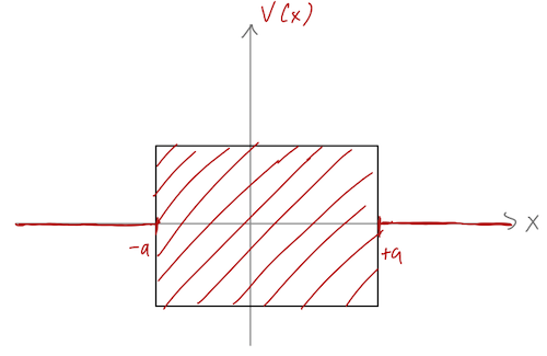
We can start by thinking about a very general case where we have a “black box” target potential near the origin; let’s say it’s an arbitrary function but still restricted to exist in the range |x| < a. We thus know that outside the black box region, we still have simple plane-wave solutions:
\psi(x) = \begin{cases} A e^{ikx} + Be^{-ikx}, & (x < -a); \\ {\rm (something\ messy)}, & (-a < x < a); \\ F e^{ikx} + Ge^{-ikx}, & (x > a). \end{cases} This is a little simplified, since we’re assuming a sharp cutoff on the black box region. If you like, you can think of the two plane-wave solutions as being asymptotic behavior for x \rightarrow \pm \infty.
We can still define the S-matrix that relates the incoming coefficients A and G to the outgoing ones B and F: \left( \begin{array}{c} F \\ B \end{array} \right) = \left( \begin{array}{cc} S_{11} & S_{12} \\ S_{21} & S_{22} \end{array} \right) \left( \begin{array}{c} A \\ G \end{array} \right). (Note that the way David Tong chooses to define his S-matrix is ever so slightly different, but nothing substantial changes in my version.) Let’s be a little more concrete about what the entries in S really are. For example, the upper row gives the relation F = S_{11} A + S_{12} G. Remember that if we introduce time dependence, A and G represent incoming particles from the left and the right respectively. We think of these coefficients as being inputs under our experimental control. If we have G=0, then S_{11} = F/A \equiv t is the ratio of transmitted to incoming amplitude - i.e. we would have for the transmission coefficient T = |t|^2. On the other hand, if we switch off A then S_{12} = F/G \equiv r' gives the reflected wave amplitude, and reflection coefficient R' = |r'|^2. (I’m using primes to distinguish the G experiment from the A experiment.)
Using this language, we can rewrite the S-matrix as {S}(k) = \left( \begin{array}{cc} t(k) & r'(k) \\ r(k) & t'(k) \end{array} \right). I’ll suppress the k dependence below to avoid clutter, but I’m writing it here to emphasize that the S-matrix consists of four numbers for each choice of wave number k. By repeated scattering experiments at different k, we can build up an arbitrarily large amount of information about the black-box region.
If we plug this back in to rewrite the wavefunction, then in terms of these coefficients we can see that \psi(x) = \begin{cases} Ae^{ikx} + (rA+t'G) e^{-ikx}, & (x < -a), \\ (tA+r'G) e^{ikx} + Ge^{-ikx}, & (x > a), \end{cases} from which we can easily read off the reflected and transmitted waves both proportional to A and to G.
There are some important constraints on the S-matrix, and therefore on the transmission and reflection parameters, that come from symmetries. First, there is simple conservation of probability. As a reminder, the probability current is given by \vec{j} = \frac{\hbar}{m} \textrm{Im} (\psi^\star \nabla \psi) and we’ve already computed it in the past for plane-wave solutions of this form (see Section 8.3): there, we found that the resulting condition is |A|^2 + |G|^2 = |B|^2 + |F|^2 which as a matrix equation, implies that S^\dagger S = 1, i.e. the S-matrix is unitary. We can use this to write out a matrix equation: {S}^\dagger {S} = \left( \begin{array}{cc} |t|^2 + |r|^2 & t^\star r' + r^\star t' \\ tr'^\star + rt'^\star & |t'|^2 + |r'|^2 \end{array} \right) = 1. From the diagonal entries, we immediately have |t|^2 + |r|^2 = |t'|^2 + |r'|^2 = 1 which is the usual statement that in either of the left-moving or right-moving experiments, we have R + T = 1; all of the incoming probability flux is either reflected or transmitted, nothing is lost. Thus, we see that a unitary S-matrix implies conservation of probability in our system, and vice-versa. The off-diagonal entries give additional conditions relating our four coefficients, but on their own they aren’t very enlightening.
However, there are two additional symmetry conditions we can add that will give us more information. The first is time reversal symmetry; we haven’t talked about this in detail, but in the present context it amounts to the condition that the black-box V(x) is real, which is true for most non-exotic Hamiltonians. Adding this condition leads to the result that t' = t, i.e. the transmitted amplitudes must be identical, and |r'| = |r| - so the reflected amplitudes have the same magnitude but can differ by a phase.
Finally, if we also have parity symmetry inside the black box, then we also find that the reflected phases must be equal, so r' = r. In the fully symmetric case, then, the entire S-matrix is characterized by just two numbers (per k value.)
Repeating the conditions and adding a bit of physical intuition:
- Conservation of probability (equivalent to S-matrix unitarity) gives us R + T = 1 for both the primed and unprimed experiments.
- A real potential in the black box (equivalent to time reversal symmetry) gives t = t' and |r'| = |r|. Intuitively, the potential doesn’t have to be symmetric so reflection can look different from the left and the right; but for transmission we pass through the entire potential, and the results must be the same from both directions.
- Finally, a parity-symmetric potential in the black box gives us r = r'; the experiments from the left and from the right are just identical.
Here I do out the algebra to show the claims I made just above. Starting with time reversal, if V(x) in the black box is real, then everything in the Schrödinger equation becomes real, which means that \psi^\star(x) is also a valid solution: \psi^\star(x) = \begin{cases} (r^\star A^\star + t'{}^\star G^\star) e^{ikx} + A^\star e^{-ikx}, & (x < a), \\ G^\star e^{ikx} + (t^\star A^\star + r'{}^\star G^\star) e^{-ikx}, & (x > a). \end{cases} You’ll notice that when we conjugate, our two “incoming” waves are now emerging from the target region; this is one way that time reversal symmetry manifests as a consequence of V(x) being real. Since this is a valid solution it must satisfy the same S-matrix equation, \left( \begin{array}{c} G^\star \\ A^\star \end{array} \right) = \left( \begin{array}{cc} t & r' \\ r & t' \end{array} \right) \left( \begin{array}{c} B^\star \\ F^\star \end{array} \right). with B = rA+t'G and F = tA + r'G from above. This is more expediently written in terms of the S-matrix again: \left( \begin{array}{c} G^\star \\ A^\star \end{array} \right) = \left( \begin{array}{cc} t & r' \\ r & t' \end{array} \right) \left( \begin{array}{cc} t'{}^\star & r^\star \\ r'{}^\star & t^\star \end{array} \right) \left( \begin{array}{c} G^\star \\ A^\star \end{array} \right), so the product of the two matrices in the middle must be the identity, \left( \begin{array}{cc} t'{}^\star t + |r'|^2 & r^\star t + t^\star r' \\ t'{}^\star r + r'{}^\star t' & |r|^2 + t{}^\star t' \end{array} \right) = 1. We can compare this to the unitarity matrix equation again: {S}^\dagger {S} = \left( \begin{array}{cc} |t|^2 + |r|^2 & t^\star r' + r^\star t' \\ tr'^\star + rt'^\star & |t'|^2 + |r'|^2 \end{array} \right) = 1. Comparing to the diagonal entries of the time-reversal matrix, we see that the transmission amplitudes must be equal, t' = t. If we take this and apply it to the off-diagonal conditions, we see that the equations in the unitary and the time-reversal condition are redundant, and they all amount to variations on the condition r' = -r^\star \frac{t}{t^\star}. So in other words, on top of the conservation of probability we already knew about, the magnitudes of the reflection and transmission coefficients are equal for left- and right-moving experiments, |r| = |r'| and |t| = |t'|. Moreover, the phase of the transmission coefficients are also equal, but the phases of the reflected amplitudes can be different.
The final symmetry that we haven’t yet considered is parity. If the black-box potential is symmetric under x \rightarrow -x, then the full Hamiltonian is parity invariant. Parity simply tells us that we can swap the left-incoming and right-incoming experiments and everything will be identical, which gives us the final condition that r' = r.
32.1.1 The S-matrix in parity basis
Since it will map nicely onto how we approach scattering in three-dimensional systems, let’s exploit parity symmetry a bit further by switching to the parity basis. This means that instead of considering left-incoming (A \neq 0), or right-incoming (G \neq 0) experiments, we instead split the system into parity-even incoming (I_e) and parity-odd incoming (I_o) experiments. Likewise, we rewrite the outgoing waves as a linear combination of parity-even (with amplitude F_e) and parity-odd (F_o). Explicitly, we can construct this as a change of basis as follows: \begin{cases} I_e &= \frac{1}{\sqrt{2}} (A+G), \\ I_o &= \frac{1}{\sqrt{2}} (-A+G), \\ \end{cases}\ \ \ \ \begin{cases} F_e &= \frac{1}{\sqrt{2}} (B+F), \\ F_o &= \frac{1}{\sqrt{2}} (B-F). \end{cases} For both the incoming and outgoing states, the basis change is given by the unitary matrix U_P = \frac{1}{\sqrt{2}} \left( \begin{array}{cc} 1 & 1 \\ -1 & 1 \end{array} \right) (you can easily verify that this is unitary, with U_P^\dagger U_P = U_P^T U_P = 1.) This gives us a different version of the S-matrix: \left( \begin{array}{c} F_e \\ F_o \end{array} \right) = S_P \left( \begin{array}{c} I_e \\ I_o \end{array} \right) with S_P = U_P S U_P^T = \left( \begin{array}{cc} t + (r + r')/2 & (r'-r)/2 \\ (r-r')/2 & t - (r+r')/2 \end{array}\right), imposing time reversal so that t=t'.
There are a couple of interesting statements we can make in this basis. First, notice that if we further impose the requirement that the black-box potential is symmetric (and thus parity-invariant), we have r=r' which gives S_P \rightarrow \left( \begin{array}{cc} t+r & 0 \\ 0 & t-r \end{array} \right) \equiv \left( \begin{array}{cc} S_e & 0 \\ 0 & S_o \end{array}\right). We see that S_P becomes diagonal due to parity symmetry; for experiments where only I_e \neq 0, we get only a parity-even output wave O_e \neq 0, and similarly for the parity-odd case. For asymmetric potentials, there is some mixing between parity-even and parity-odd states, captured entirely in the difference r'-r.
We also know that there are further constraints on S_e and S_o from other symmetries. In particular, if we square them, |S_e|^2 = |t+r|^2 = |t|^2 + |r|^2 + r^\star t + t^\star r \\ |S_o|^2 = |t-r|^2 = |t|^2 + |r|^2 - r^\star t - t^\star r But unitarity above gave us the condition that r^\star t + t^\star r = 0, so we have |S_e|^2 = |S_o|^2 = 1. In other words, the S-matrix in parity basis for a symmetric potential is given by two phase shifts, written conventionally as S_P(k) = \left( \begin{array}{cc} e^{2i\delta_e(k)} & 0 \\ 0 & e^{2i\delta_o(k)} \end{array} \right). Measuring how the phases of our outgoing and incoming waves compare as a function of momentum is thus all we need in order to probe the black-box potential.
32.2 The S-matrix and bound states
There is an enormous amount of useful information encoded in the S-matrix, which as we’ve emphasized is a function of the scattering momentum k. As long as E > 0 we know that k will be real; as k \rightarrow \infty, we expect that {S}(k) goes to the identity matrix, since for a sufficiently energetic particle the potential will have little effect and we expect the transmission coefficient T \rightarrow 1.
What about the case where E < 0? At first glance this would seem to have nothing to do with the S-matrix, because the plane-wave form of our solutions to the Schrödinger equation becomes invalid at asymptotic x. However, that’s not entirely true: from a mathematical point of view, the Schrödinger equation in regions where V=0 simply looks like \psi''(x) = -\frac{2mE}{\hbar^2} \psi(x) = -k^2 \psi(x) where the latter definition is still perfectly fine if E < 0, as long as we allow k to be imaginary. If k \equiv i\kappa where \kappa is real, then we have for our asymptotic solutions \psi(x) = \begin{cases} Ae^{-\kappa x} + (r(k)A+t'(k)G) e^{\kappa x}, & (x \rightarrow -\infty); \\ (t(k)A+r'(k)G) e^{-\kappa x} + Ge^{\kappa x}, & (x \rightarrow +\infty). \end{cases}
We see a problem right away: two of the exponential solutions blow up at infinite x and are not normalizable! The appropriate limit to remove the divergent parts of our solutions is A, G \rightarrow 0. But then since A and G appear in every term in the solution, we seem to have no solution left: \psi(x) = 0 everywhere. But there is another option: if r(k)A and t(k)A remain finite as A \rightarrow 0, then the well-behaved real exponentials can be non-zero, as in the bound-state solutions that we expect to find. This means that the S-matrix entries themselves must diverge at the values of k corresponding to bound states.
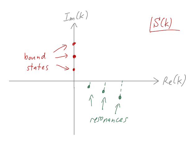
In other words, thinking of {S}(k) as a function of the complex wave number k, the behavior of {S}(k) along the real axis tells us about asymptotic scattering states with positive energy, but we can get even more: bound states can be identified as poles of {S}(k) along the imaginary axis.
You might complain that talking about poles of a matrix is imprecise; if you like, the correspondence is with poles in the eigenvalues of {S}(k), in general. To be more concrete, we can specialize to a symmetric potential and work in the parity basis, where we know that S(k) = \left( \begin{array}{cc} e^{2i\delta_e(k)} & 0 \\ 0 & e^{2i\delta_o(k)} \end{array} \right). Here we have a simple diagonal matrix, and the interpretation is clear: along the real axis, the phase shifts \delta(k) should remain finite, encoding information about the scattering potential V(x). On the imaginary axis, S(i\kappa), the poles in \delta(k) correspond to bound-state solutions, and away from these special values of k no solutions to the scattering problem occur.
32.2.1 Resonances
The fact that both the real and imaginary parts of S(k) contain interesting physics information about a given potential should make us wonder whether there is anything else interesting hidden in the complete structure of S(k) continued into the complex plane. In fact, there is: the phenomenon of resonance can be understood in terms of poles structure at complex k.
It’s easiest to understand this part of the discussion if we work backwards. Assume that S(k) has a pole at the complex value k_0 - i \gamma, where \gamma > 0 (this will turn out to be the interesting case.) We can work backwards to obtain the energy of the state from k: E = \frac{\hbar^2 k^2}{2m} = \frac{\hbar^2 (k_0^2 - \gamma^2)}{2m} - 2i \frac{\hbar^2 \gamma k_0}{2m} \equiv E_0 - \frac{i\Gamma}{2}. So the energy is complex. Your first reaction might be “obviously this is unrealistic” - either because you know on physical grounds that energy should be real, or because we’ve said the Hamiltonian is Hermitian and so its eigenvalues should be real. But let’s ignore that for the moment and ask what a complex energy might mean. The simplest way to understand what’s happening is to consider the time-dependence of such a state: we will have \psi(x,t) \sim e^{-iEt/\hbar} \psi(x) = e^{-iE_0 t/\hbar} e^{-\Gamma t/2\hbar} \psi(x). In addition to the usual phase, we have exponential decay of the entire state! We would similarly find that the probability density is decaying exponentially. To think about asymptotic behavior in this case, it’s helpful to restore the spatial dependence: for example, for the transmitted part of the solution as x \rightarrow \infty, we have \psi(x,t) \sim e^{ikx} e^{-iEt/\hbar} = e^{ik_0 x} e^{-iE_0 t/\hbar} \exp \left[ \gamma x - \frac{\Gamma t}{2\hbar}\right] \\ = (...) \exp \left[ \gamma (x - vt) \right], where v = \frac{\Gamma}{2\hbar \gamma} = \frac{\hbar k_0}{m} is the linear speed determined by the (real) energy and mass of our particle. We see that in addition to the usual plane-wave oscillations, there is an exponential profile, but more importantly, that profile is translating to the right at speed v. (We’ll find a similar solution on the left.)
We’ve now seen enough math to assign a physical interpretation. As we discussed above, poles in S(k) indicate the energy values that correspond to bound states. These are generally on the imaginary-k axis, corresponding to E<0, since the solution must not exist asymptotically for the particle to be truly bound. But we could easily imagine a potential which consists of a large and deep well, but not an infinitely deep one:
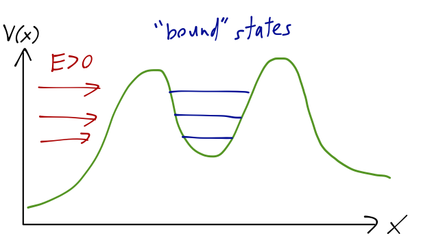
We might expect to find “bound states” here if the well is deep and wide enough and we ignore the outside. But the presence of the lower-energy region outside the well means any such states must be unstable! If we imagine an initial state with our particle trapped inside the well, it will have some finite probability per unit time to tunnel through the barrier and escape; if we wait long enough, it will definitely escape. This is exactly the situation described by a complex energy eigenvalue above: the local wavefunction \psi(x,t) within the well decays exponentially to zero, and the wavefront outside the well moves away with some linear speed.
The energy levels inside the well are also known as resonances. They can indeed be identified as complex poles in the S-matrix. Of course, if we probe the well by carrying out a scattering experiment and measuring the transmission coefficient T, we will only be studying S(k) on the positive real axis, so we will never see a divergence in T. However, it’s easy to see that the presence of nearby complex poles will cause local maxima in T - precisely the phenomenon of transmission resonance that we noted before.
Note that this whole explanation requires \gamma > 0, i.e. the poles to be in the lower half-plane; otherwise we would have exponential growth with \Gamma instead of decay, which would not match on to this experimental situation anymore.
We can go a step further and see precisely how a pole would cause a transmission resonance. Let’s think in terms of energy instead of k this time: suppose the transmission amplitude t(E) has a pole at E = E_0 - i\Gamma/2 as above. Close enough to the pole, it will dominate over all other contributions: t(E) \approx \frac{Z}{E - E_0 + i\Gamma/2}, where Z is the residue of the pole. The transmission coefficient for real E is then equal to T(E) \approx \frac{|Z|^2}{(E-E_0)^2 + \Gamma^2/4}. This should look familiar: this is exactly the same Lorentzian distribution that we saw in our discussion of line widths. The peak is at E_0, and the parameter \Gamma is known as the width of the Lorentzian, because it corresponds to the width of the peak (strictly, the “full-width at half-max”, i.e. the distance between the points halfway down from the peak):
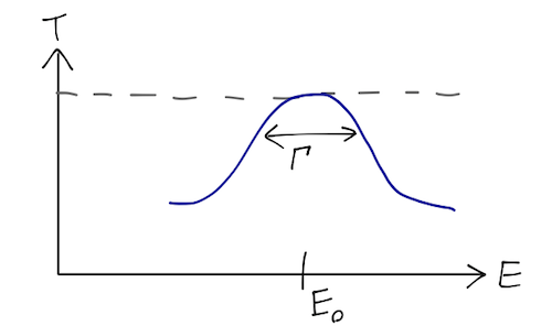
The Lorentzian isn’t always a great approximation, depending on how far away the closest pole is and how many other poles are nearby, but it always works if we’re “close enough” to a single pole.
I’ll emphasize once again that actually interpreting complex energies as “physical” states is a phenomenological concept. Strictly speaking, in quantum mechanics probability is conserved, Hamiltonians are Hermitian, and there are no complex energy eigenvalues. But if we look at a local part of a whole system, like the inside of a potential well, then we can approximate the behavior by making use of complex energies. Probability conservation is lost, but just because we’ve restricted our attention - we know the lost probability flows out of the well and into asymptotic states.
32.3 Example: The potential step and the S-matrix
Now that we’ve set up the formalism, we’re ready to see the payoff in terms of physics understanding in an example system. Let’s do a unified treatment of the well and the barrier that I’ll call the potential step, where we have constant V_0 for |x| < a but the sign of V_0 is left arbitrary. We can write the general solution as \psi(x) = \begin{cases} A e^{ikx} + Be^{-ikx}, & (x < -a); \\ C e^{ik'x} + De^{-ik'x}, & (-a < x < a); \\ F e^{ikx} + Ge^{-ikx}, & (x > a). \end{cases} where k = \sqrt{2mE} / \hbar and k' = \sqrt{2m(E-V_0)} / \hbar will be complex in general. They are, of course, not independent - we recognize immediately that k'^2 = \frac{2m(E-V_0)}{\hbar^2} = k^2 - \frac{2mV_0}{\hbar^2}.
At the left boundary, we have the equations A e^{-ika} + Be^{ika} = Ce^{-ik'a} + De^{ik'a} \\ kA e^{-ika} - kBe^{ika} = k'C e^{-ik'a} - k'D e^{ik'a} and at the right boundary, C e^{ik'a} + De^{-ik'a} = Fe^{ika} + Ge^{-ika} \\ k'C e^{ik'a} - k'D e^{-ik'a} = kFe^{ika} - kGe^{-ika}
We can brute-force the algebra in Mathematica for this problem; the expressions are messy but not intractible. However, since this is a symmetric potential it’s actually much nicer to switch to the parity basis, at which point we can work things out by hand. Let’s calculate the two matrix elements one at a time, first turning only the even-parity incoming wave, so I_o = 0. This means that A = G = I_e / \sqrt{2}, and B = F = F_e / \sqrt{2}. Because we’re selecting a parity-even solution, \psi(x) should be even under parity, which also tells us that in the middle region we must have C = D. Finally, parity guarantees that the left and right boundaries will give us the same equations, so let’s just focus on the left boundary: I_e e^{-ika} + F_e e^{ika} = 2\sqrt{2} C \cos (k' a), \\ I_e e^{-ika} - F_e e^{ika} = 2\sqrt{2} \frac{-iCk'}{k} \sin(k' a), or dividing through to cancel C off, \frac{I_e e^{-2ika} - F_e}{I_e e^{-2ika} + F_e} = \frac{-ik'}{k} \tan(k'a). Let’s solve for F_e; reorganizing a bit, I_e e^{-2ika} (1 + \frac{ik'}{k} \tan(k'a) ) = F_e (1 - \frac{ik'}{k} \tan(k'a)) \\ \Rightarrow S_e = \frac{F_e}{I_e} = e^{-2ika} \frac{k + ik' \tan(k'a)}{k - ik' \tan(k'a)}. Let’s check a couple of limits: if we take a \rightarrow 0 then S_e = 1, so the incoming wave isn’t affected at all. Similarly in the limit E \rightarrow \infty or V_0 \rightarrow 0 we would have k = k', and we find I_e \rightarrow e^{-2ika} \frac{\cos(ka) + i \sin(ka)}{\cos(ka) - i \sin(ka)} = e^{-2ika} (e^{2ika}) = 1 as expected (if E is very large the presence of the step doesn’t disturb the incoming wave either.) As one more check, you can easily verify that S_e is a pure phase as expected, i.e. |S_e|^2 = 1.
For S_o, the equations are almost identical except that for an odd-parity solution, we instead have C = -D in the middle region. This results in the equation \frac{I_o e^{-2ika} - F_o}{I_o e^{-2ika} + F_o} = \frac{ik'}{k} \cot(k'a) which leads to S_o = e^{-2ika} \frac{k - ik' \cot(k'a)}{k + ik' \cot(k'a)}.
Converting these to phase shifts is a bit non-trivial, but it also isn’t necessary; we now have everything we need to study the structure of the S-matrix in the complex plane. By inspection, we see that the even and odd S-matrix elements respectively have poles in the complex plane at the positions k = ik' \tan k'a,\ \ k = -ik' \cot k'a. These right-hand sides are pure imaginary; if E > 0, then k is real and there are no poles in the transmission coefficient (good news!) On the other hand, if E < 0 we have poles that we know should correspond to bound states, and indeed we recover exactly the bound-state energy equations that we found previously (see Section 8.5), e.g. \eta = \xi \tan \xi!
What about the other possibility, that k' is pure imaginary? (This corresponds to the case E < V_0.) If we identify k' = i \kappa, then instead we find the two equations k = -\kappa \tanh \kappa a,\ \ k = -\kappa \coth \kappa a.
In the k plane, these solutions must lie somewhere on the negative real axis; but since k is the square root of the (real) energy, it’s either real and positive or imaginary and positive. (Letting k be negative will amount to flipping which solutions we think of as incoming and outgoing, which invalidates some assumptions we’ve made.) So there are no poles in the case of the potential barrier, which is good because a pole in the transmission coefficient with visible asymptotic states at x = \pm \infty would violate probability conservation badly!
We know that we can actually generalize completely to allow k to be in the complex plane. Finding the complex pole locations is not easy, so I will resort to a numerical treatment: we can plot t(k) in the complex plane for some simple numerical values a = 1, m = 1, and V_0 = \pm 1. Here’s what we see:
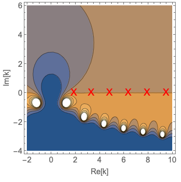
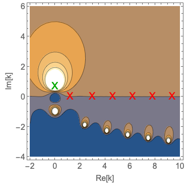
I’ve put the locations of the transmission resonances (where |T| = 1, we’ve looked at these before) for positive/negative V_0 on the real axis (red X’s), and the first bound-state energy solution for negative potential on the imaginary axis in the right plot (green X). We see that everything lines up pretty well! (The transmission resonances are not perfectly above the poles, but since the poles are relatively close together we wouldn’t expect them to be; imagine adding together a sequence of increasingly broad Lorentzian curves.)