1 Introduction
Since this is a graduate course, I don’t really need to begin by motivating quantum mechanics; you all know that we live in a fundamentally quantum world. No matter what topics your undergraduate physics education emphasized, you are certainly aware of concepts like particle-wave duality and the crucial role of probability in quantum mechanics.
However, there are some important ideas at the core of quantum mechanics which fight against human intuition. Your undergraduate quantum course may have emphasized wave mechanics, focusing on the wavefunction and the Schrödinger equation. There is certainly nothing wrong with such an approach; I could teach an entire semester-long graduate course with nothing but wave mechanics (as in the excellent book by Merzbacher), and we would learn a lot of physics. But the wave mechanics picture alone is incomplete; to understand many important quantum phenomena, we need the more abstract idea of a Hilbert space, which is a vector space with some additional properties.
To be more concrete, the language of Hilbert spaces will let us fill in two huge gaps from wave mechanics:
- Finite-dimensional spaces - the wavefunction is a continuous distribution, but some important quantum systems only have a finite number of states, e.g. spin.
- Operators - translating classical observables into ``operators’’ (promoting momentum p to the momentum operator \hat{p} = -i\hbar (d/dx), for example) is a mysterious procedure, and not every quantum observable has a classical starting point (once again, spin turns out to be a good example.)
In addition to all of the above benefits, the Hilbert space approach has the benefit of giving us deeper understanding in cases where we can’t simply write down and solve an equation - outside of a handful of exactly-solvable and famous examples, solving the Schrödinger equation is usually not tractable!
The formalism of Hilbert space will allow us to describe wave mechanics as well, but describing a continuous wavefunction in this way will require wrapping our heads around infinite-dimensional vectors. So to make the introduction of Hilbert spaces slightly gentler, we’ll begin with some finite-dimensional examples before we return to see how wave mechanics fits in.
1.1 The double-slit experiment
The double-slit experiment is a classic example of particle-wave duality. The setup is simple: a barrier with two gaps in it, a source, and a detector. I presume you have all seen this before, so I’ll just remind you of the punchline - if we conduct the experiment with low-intensity light, or with electrons, we see a characteristic interference pattern:
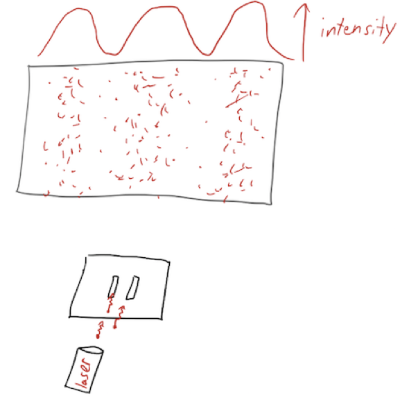
But at the same time, we can still see individual counts from the particles passing through the slits one at a time. So electrons are particles - we clearly see their individual impacts on the screen - and they are waves, as evidenced by the interference pattern that builds up.
Richard Feynman, who played a large role in promoting the double-slit experiment using electrons and its variations, called it “the heart of quantum mechanics”; you’ll find a more detailed treatment, including lots of interesting variations on the experiment, in the Feynman lectures. By the way, if you’ve never seen a video of this experiment with single photons, you should watch it (you can start around 6:50 if you just want to see the pattern): https://www.youtube.com/watch?v=I9Ab8BLW3kA#t=6m50s.
1.2 The Stern-Gerlach experiment
Although I don’t want to spend too much time on broad motivation, let’s begin with one specific example, the Stern-Gerlach experiment. This example, which Sakurai also begins with, will help to motivate the study of finite-dimensional Hilbert spaces in particular. I also like starting with experiment because a lot of quantum mechanics is very weird and counter-intuitive, and it’s nice to see explicitly that it isn’t just because theoretical physicists like cooking up strange theories: we are forced to confront the quantum nature of reality even by careful study of a simple experiment like this. For an even more in-depth study of this system and its implications, you should refer to the Feynman Lectures on Physics.
We start with a beam of atoms - let’s say silver atoms specifically, since silver has a single unbound valence electron, which makes it act like a very heavy, neutral, free electron. In particular, the magnetic moment \boldsymbol{\mu} of the silver atom is the same as the magnetic moment of an electron. The experiment we want to consider is based on interaction with the magnetic moment:
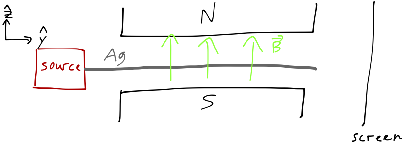
We pass our beam of silver atoms through a magnetic field, oriented in the \hat{z} direction as pictured, and then look for their locations on a distant screen in the \hat{y} direction. As you may remember, the potential energy of a magnetic moment interacting with a magnetic field \mathbf{B} is equal to U = -\boldsymbol{\mu} \cdot \mathbf{B}, so that the silver atoms will feel a force in the \hat{z} direction, \mathbf{F}_z = \frac{\partial}{\partial z} (\boldsymbol{\mu} \cdot \mathbf{B}) \approx \mu_z \frac{\partial B_z}{\partial z}, assuming the other components of the \mathbf{B}-field are negligible. (Note that this requires a non-uniform B_z, which explains the funny spiked shape of a Stern-Gerlach apparatus if you look at a real one.) We assume the experiment is large enough that the displacement of the atoms can be treated classically.
Although it’s not essential to understand the experiment, it’s useful to point out that the magnetic moment of a particle is proportional to its spin, \boldsymbol{\mu} \propto \boldsymbol{S}. This makes some amount of intuitive sense; if a classical ball of charge is spinning, it will generate a magnetic moment proportional to its angular velocity vector. There are some good reasons not to take this mental picture too literally for real quantum spin - in particular, there is no sensible way to interpret the electron’s spin as rotating charge once we get into the details. But I will still frame the rest of the example in terms of spin rather than magnetic moment, to be more in-line with other standard treatments and since spin is a little more intuitive as a property of a particle.
Now, if the silver atoms behave like classical objects, then we should expect the z component of their spins to vary between -|\mathbf{S}| and +|\mathbf{S}| continuously, corresponding to a random distribution for the axes of the spin vectors coming from the source. This would give us a continuous band of impacts on the screen between the two extreme values. What we actually see is two well-separated spots:
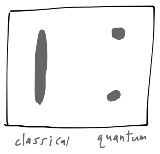
The position of the spots allows us to work backwards to determine the \hat{z}-component of the atomic spin: S_z = \pm \hbar/2. So the atom’s spin cannot vary continuously, it is quantized to two discrete values. (The magnitude is irrelevant for the rest of discussion, so I’ll just say S_z = \pm.) This is a fundamentally quantum phenomenon; the name “quantum” comes from quantization, which was at the heart of early quantum models such as Bohr’s atomic model.
We can declare success at this point, but it’s worth going a little further to appreciate some of the weirdness of the quantum world that goes beyond just quantization. Based on the results above, we can think of a single Stern-Gerlach apparatus as a box that splits an incoming beam into two outgoing ones which are pure spin-up (S_z = +) or spin-down (S_z = -) atoms. A second S-G apparatus in the \hat{z} direction is found to have no additional effect; we see only a single spot corresponding to the unblocked component.
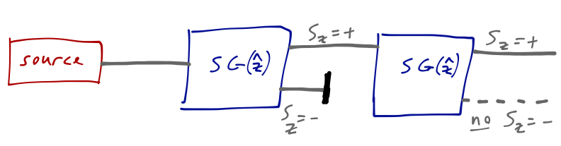
This is just confirming that the first apparatus produced a beam of S_z = + atoms. If we now rotate the second magnet so that it points in the \hat{x} direction, then we once again see two spots on the screen, corresponding to S_x = + and S_x = -.
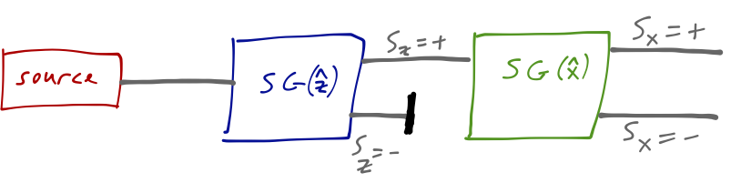
The intensity of the two spots is equal, as in the single S-G experiment. But we’ve now filtered on both S_z and S_x. If we take the top beam here, does that mean that it is a pure beam containing atoms with both S_z = + and S_x = +? To find out, we add another S-G apparatus in the \hat{z} direction, and we find something truly surprising: two spots, corresponding to S_z = \pm!
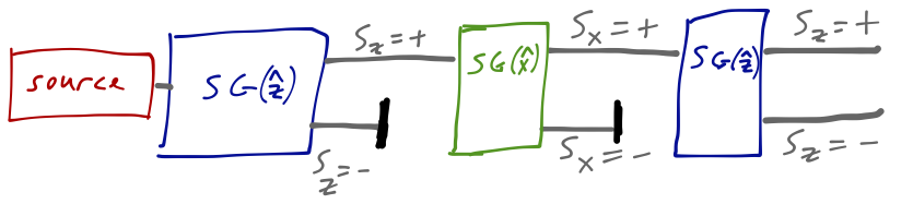
Even though we blocked the S_z = - component, it has returned simply due to the presence of the \hat{x}-oriented magnet in the middle! This tells us that the atoms coming out of the second S-G experiment can’t just be thought of as having their spins oriented in a definite direction; somehow, the projection onto the S_x components has removed the ``memory’’ of the first S_z = + projection.
You could object that this experiment on its own isn’t ironclad proof of quantum behavior: after all, a magnetic field in the \hat{x} direction will cause the precession of a classical magnetic moment around the \hat{z} axis. Of course, describing this effect using a classical theory would be difficult since the two-point distribution that comes out of the S-G is already at odds with the classical idea of a spin vector moving continuously around in space.
At any rate, we can avoid this complication by being more careful about the experimental setup; for example, in the Feynman lectures he considers an ``improved S-G device” which consists of two back-to-back Stern-Gerlach devices that have opposite orientation, so that the beams are brought back together. We then put in the blocks internally, between the two devices. In the improved device, any precession from the first device will be reversed by the second one.
In these notes I haven’t bothered to do this since we’re not too concerned with the experimental details; this is just a pedagogical example. But the question occurred to me when writing this, so I thought I’d include it as an aside.
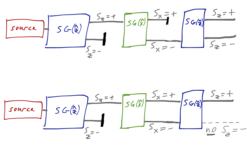
Let’s consider two more similar experiments. In the top configuration, we block the S_z = + component; the outcome from the final \hat{z} device is the same. But if we unblock both components and then recombine, then the effect of the middle S-G apparatus is to do nothing at all.
But now we have something really interesting! Immediately, we see signs of an interference effect: removing the blocks in the middle (and so increasing the number of atoms passing through the experiment) has decreased the number of atoms coming out of the end with S_z = -. We can see this concretely by writing the conditional probabilities for atoms in the final S_z = - state: p(S_z = -) = p(S_z = - | S_x = +) p(S_x = +) + p(S_z = - | S_x = -) p(S_x = -)
(here I’m focusing on what happens when we change the blocks in the middle apparatus, so I’m ignore the fact that the initial state was S_z = + from the very beginning.) Every number on the right-hand side of this equation is 50%, from the other versions of the experiment above. But the left-hand side, experimentally, is zero! We see that our quantum theory of probability and events must be somewhat different than the classical theory, and indeed we will find that in quantum mechanics there is a third term in the equation above due to interference that cancels the other two.
There’s one more essential ingredient of quantum mechanics that we are forced to adopt by going a little further with Stern-Gerlach experiments. Since the outcome of a Stern-Gerlach experiment is binary (spin-up or spin-down), we can use a two-dimensional vector space to represent the states. For example, we can use the \hat{z} direction experiment to establish basis vectors, S_z = + \Rightarrow \left(\begin{array}{c}1\\0\end{array}\right) \\ S_z = - \Rightarrow \left(\begin{array}{c}0\\1\end{array}\right). Given this choice, to reproduce all experimental results the S_x spin orientations should be expressed as S_x = + \Rightarrow \frac{1}{\sqrt{2}} \left(\begin{array}{c}1\\1\end{array}\right) \\ S_x = - \Rightarrow \frac{1}{\sqrt{2}} \left(\begin{array}{c}-1\\1\end{array}\right) In this abstract vector space, passing our beam through a Stern-Gerlach device and blocking one of the output components is exactly a projection along the given direction. It’s easy to see in these terms that even after projecting only the S_z = + component out, the subsequent projection on the S_x = + direction will have both \hat{z} spin components present.
But we’ve been forgetting about the third direction, S_y. There should be nothing special about the \hat{x} direction versus \hat{y}, of course - and indeed if we run the experiment above using \hat{y} instead of \hat{x}, we get the same results. In fact, if you pick any two of \{\hat{x}, \hat{y}, \hat{z}\} and run experiments like we did above, you’ll get the same results. However, it seems like we’ve used up our mathematical freedom in defining the S_x states. If you try, you’ll quickly realize that the only way out is to enlarge the space by allowing the vector components to be complex; then we can write S_y = \pm \hbar/2 \Rightarrow \frac{1}{\sqrt{2}} \left(\begin{array}{c}1\\ \pm i\end{array}\right) and reproduce all possible combinations of Stern-Gerlach experiments.
Another reasonable objection you could make to the argument so far is that we didn’t need complex numbers; the only thing that we’ve argued is that we definitely need more than two independent degrees of freedom to describe the Stern-Gerlach system. Going to two complex numbers is one way to solve this, but we could also have tried to describe the results using a larger number of real dimensions instead.
In fact, while it is possible to do so for this limited example, we will eventually run into inconsistencies if we try to define a purely real quantum theory; in particular, we will find that we end up with the wrong number of dimensions again when we try to relate single-particle to multi-particle quantum systems. The way in which these inconsistencies manifest is subtle, but if you’re interested in more, see this Physics Today article. In these notes we’ll continue with the standard complex approach, and not worry about possible real-number formulations.
To summarize, in the Stern-Gerlach experiment, we’ve found three essential ingredients to describe the physics of reality:
- Quantization;
- Interference;
- Complex numbers.
All of this is just a motivation for how we will write down quantum mechanics as a theory; if you’re puzzled, read the discussion in Sakurai, which also includes a discussion of polarization of light which you may find helpful.