25 Propagators and path integration
As far as time evolution in quantum mechanics goes, we’ve seen a fair amount of formalism by now, but a lot of it has focused on evolution of quantum states. While this is technically all that we need to study any quantum system, it will be useful to focus a bit more specifically on time evolution for particles propagating in space. This will lead us to some very useful tools: the propagator, and the path integral.
25.1 Warm-up: propagation of plane waves
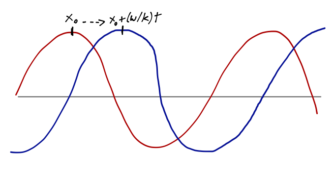
Let’s begin by reminding ourselves of how time evolution works for simple, free solutions in quantum mechanics: that is, solutions where the potential is V(\hat{x}) = 0, so the Hamiltonian is \hat{H} = \hat{p}^2 / 2m. Our energy eigenstate solutions, which are also momentum eigenstates, are plane waves: \psi_E(x) = Ae^{ikx} + Be^{-ikx} where the wave number k = p/\hbar. Acting with the time evolution operator gives us an overall phase since this is an energy eigenstate, \psi_E(x,t) = \bra{x} \exp \left( \frac{-i \hat{H} t}{\hbar} \right) \ket{\psi} = e^{-iEt/\hbar} \left\langle x | \psi \right\rangle \\ = A e^{i(kx-\omega t)} + Be^{-i(kx+\omega t)}, with \omega = E/\hbar. Overall, each plane wave is represented as a pure phase, e^{i\phi(x,t)}. Moreover, we see that the value of the phase repeats in time, e.g. for wave A: kx = k\left(x+\frac{\omega}{k} t \right) - \omega t \\ \Rightarrow \phi_A(x,0) = \phi_A(x+\frac{\omega}{k} t,t). We identify v_p \equiv \omega / k as the phase velocity associated with our (right-moving) plane wave, A. Similarly, wave B moves to the left with the same phase velocity.
As implied by thinking about “right-moving” versus “left-moving”, a plane wave clearly represents a moving particle, in some way. This seems to match nicely onto the descriptions of the two plane-wave solutions as momentum eigenstates: acting with \hat{p} = -i\hbar \partial / \partial x we easily see that e^{ikx} is a momentum eigenstate with p = \hbar k, and similarly p = -\hbar k for the left-moving wave.
However, we notice something odd if we plug in the dispersion relation (energy-momentum relation) for a free particle to find the phase velocity: E(k) = \frac{\hbar^2 k^2}{2m} = \hbar \omega \\ \Rightarrow v_p = \frac{\omega}{k} = \frac{\hbar k}{2m} = \frac{p}{2m}. This is only half of the classical momentum of a single particle! Why is there a discrepancy?
We have to remember that a plane wave is something of an odd object. For simplicity I will set B=0 and focus on a right-moving plane wave. If we’re going to try to do an experiment to find out the velocity of our particle, we have to measure its position at successive times: Born’s rule tells us that the probability of any outcome is p(x) = \int_{-\infty}^\infty dx' \delta(x-x') |\psi(x',t)|^2 = |\psi(x,t)|^2. But for a plane wave, |\psi(x,t)|^2 is a constant, A^2! So we’re equally likely to find our particle anywhere, at any t, regardless of the phase velocity. Thus we shouldn’t be worried that the phase velocity doesn’t equal the classical velocity, because the phase velocity clearly doesn’t have the same physical meaning. (I am not aware of any good explanation of why it should be precisely half of the classical velocity, but at least the fact that it is different from the classical velocity shouldn’t bother us.)
25.2 Propagation of wave packets and dispersion
To make a proper comparison with the classical velocity of a particle, we have to start with a more localized state; a natural candidate is the wave packet, which we met before as a minimum-uncertainty solution to the free Hamiltonian. Given the parameters x_0, k_0, and \Delta x, the wave packet solution is \psi(x,0) \propto \exp \left( ik_0 x - \frac{(x-x_0)^2}{4(\Delta x)^2} \right) As we’ve seen before, this looks like plane wave multiplied by a Gaussian “envelope”; the probability density |\psi(x,0)|^2 is pure Gaussian, centered at x_0 and with width (\Delta x). If we take the Fourier transform of a Gaussian, we find another Gaussian in momentum space: \tilde{\psi}(k,0) = \frac{1}{\sqrt{2\pi}} \int_{-\infty}^\infty dx\ \psi(x,0) e^{-ikx} \\ \propto \exp \left[ -ik x_0 - \frac{(k-k_0)^2}{4(\Delta k)^2} \right]. where \Delta k = 1 / (2 \Delta x).
We have seen before in Section 5.4 that the wave packet is a (minimum-uncertainty) solution to the free Hamiltonian. However, it’s actually a useful wavefunction in a much more general context, which is any system for which there is a dispersion relation. A dispersion relation is a function E(k) (or equivalently, \omega(k) = E(k) / \hbar) that relates energy to wave number. Obviously for this relation to be sensible, it has to be true that our energy eigenstates can also be labelled by their wave number (i.e. momentum). Since momentum is the generator of translation, this means that dispersion relations occur in systems which preserve translation symmetry in some form. This can take several forms:
- The free Hamiltonian \hat{H} = \hat{p}^2 / (2m) satisfies [\hat{H}, \hat{p}] = 0, so it is fully translation invariant, and the energy eigenstates are momentum eigenstates.
- Any Hamiltonian which preserves finite translations, [\hat{H}, \hat{\tau}(L)] = 0, satisfies a dispersion relation with restricted values of k allowed as per Bloch’s theorem (see Section 10.2).
- If our wave packet width \Delta x is very narrow compared to the scale over which the potential V(x) varies, then translations can be approximately conserved, so that we can usefully write an approximate, local dispersion relation E(k).
We’ll proceed from here without assuming anything about what Hamiltonian we’re considering, except that it should have some undetermined dispersion relation E(k). Since this means that momentum eigenstates are also energy eigenstates, the time evolution of the wave packet is simple to write down since it’s built as a linear combination of momentum states: \tilde{\psi}(k,t) = \left\langle k | \psi(t) \right\rangle = \bra{k} e^{-i\hat{H} t/\hbar} \ket{\psi(0)} = e^{-i\omega(k) t} \tilde{\psi}(k,0). Fourier transforming back to position space, the time-evolved wave packet is thus \psi(x,t) = \frac{1}{\sqrt{2\pi}} \int_{-\infty}^\infty dk\ \exp \left[ -ikx_0 - \frac{(k-k_0)^2}{4(\Delta k)^2} \right] e^{i \phi(k)} where I’ve defined the phase \phi(k) = kx - \omega(k) t. If the dispersion relation is totally general, then we have to stop here; but since our wave packet is sharply peaked around k=k_0, let’s try to do a Taylor expansion of the phase \phi(k) about the same point: \phi(k) \approx \phi_0 + \phi'_0 (k-k_0) + \frac{1}{2} \phi''_0 (k-k_0)^2 where \phi_0 = k_0 x - \omega_0 t \\ \phi'_0 = \left. \frac{d\phi}{dk} \right|_{k=k_0} = x - \frac{d\omega}{dk} t \\ \equiv x - v_g t \\ \phi''_0 = \left. \frac{d^2 \phi}{dk^2} \right|_{k=k_0} = -\frac{d^2 \omega}{dk^2} t \\ \equiv -\alpha t. Plugging back in, we find \psi(x,t) \propto e^{i (k_0 x - \omega_0 t)} \int_{-\infty}^\infty dk\ \exp \left[ i(k-k_0) \left( x-x_0 - v_g t\right) - (k-k_0)^2 \left( \frac{1}{4(\Delta k)^2} + i \alpha t \right) \right].
You’ll recognize this as a Gaussian integral; with some appropriate changes of variables we can reduce the integrand to something of the form e^{-u^2} and then do it. I’ll just tell you the result, up to normalizing constants that I’ve been ignoring anyway: \psi(x,t) \propto \exp \left[ i(k_0 x - \omega_0 t) - (x-x_0 - v_g t)^2 \frac{1 - 2\alpha i (\Delta k)^2 t }{4\sigma(t)^2} \right]. with \sigma^2(t) = (\Delta x)^2 + \frac{\alpha^2 t^2}{4 (\Delta x)^2}. At t=0 this reduces to our original formula for the wave packet, which is a good cross-check. This formula is a little intimidating, but if we square it to find the probability density for finding our particle at position x, it becomes illuminating: |\psi(x,t)|^2 \propto \frac{1}{\sigma(t)} \exp \left[ -\frac{(x-x_0 - v_g t)^2}{2 \sigma^2(t)} \right]. This is, once again, a Gaussian distribution, but with the peak translated from x_0 to x_0 + v_g t. So the constant v_g = d\omega / dk is exactly what we should interpret as the analogue of the classical speed of our particle; it determines the rate at which the most likely outcome of measuring x changes. v_g is called the group velocity. It’s easy to check that the dispersion relation for a free particle gives us v_g = \frac{\hbar k}{m} = \frac{p}{m}, matching on to the classical expectation. So to summarize, the center of a wave packet travels at the group velocity v_g = d\omega / dk, while the phase of a plane wave changes with the phase velocity v_p = \omega / k. The wave packet is the closest analogue to a classical experiment involving a single particle; a plane wave is better thought of as a continuous stream of particles moving in one direction.
One other observation we can make from our result for the evolution of a wave packet is that although it remains Gaussian, the width of the packet \sigma(t) increases over time, according to the constant \alpha = d^2 \omega / dk^2, which is commonly called the “group velocity dispersion” or sometimes just “the dispersion”. Since \sigma(t) \sim \alpha^2, you can see that whatever the sign of \alpha, the wave packet will spread out over time; for example, for the free particle we have \alpha_{\rm free} = \frac{\hbar}{m}.
The only exception to the spreading of wave packets occurs when \alpha = 0. This is the case for systems with linear dispersion relations, \omega(k) = ck; light waves are one example. Linear dispersion also leads to the property that v_p = v_g, e.g. light waves and light pulses travel at the same speed, c.
25.3 Time evolution and propagators
Note that in the below, I’m going to almost always work with a single spatial dimension, in order to make definitions and derivations a little bit simpler. Generalizing the propagator and related concepts to three dimensions is simple: just replace x \rightarrow \vec{x} and make any other needed adjustments that result (normalization of things like Fourier transforms, and delta functions go from \delta(x-x') \rightarrow \delta^{(3)}(\vec{x} - \vec{x}'), for example.)
Our method for finding the time evolution of the wave packet points us towards a more general procedure that we can use for time evolution of any wavefunction. Now we want to be as general as possible, so we no longer assume that momentum commutes with the Hamiltonian. Given some completely arbitrary initial state, we know that the time evolution can be written as \ket{\psi(t)} = \exp \left[ -\frac{i \hat{H} (t-t_0)}{\hbar} \right] \ket{\psi(t_0)}. We can rewrite this fully in position space by dotting in a position eigenstate from the left, and also inserting a complete set of position states, to get the following: \left\langle x' | \psi(t) \right\rangle = \int dx\ \bra{x'} \exp \left[ -\frac{i \hat{H} (t-t_0)}{\hbar} \right] \ket{x} \left\langle x | \psi(t_0) \right\rangle \\ \equiv \int dx K(x', t; x, t_0) \psi(x, t_0), defining the kernel function K, also known as the propagator, K(x', t; x, t_0) \equiv \bra{x'} \exp \left[ -\frac{i\hat{H} (t-t_0)}{\hbar} \right] \ket{x}.
In the limit t \rightarrow t_0, the operator in the middle approaches the identity, so we find simply \lim_{t \rightarrow t_0} K(x', t; x, t_0) = \delta(x'-x).
Treating the propagator as a wavefunction itself, it’s straightforward to show that it is a solution to the Schrödinger equation: \left[ - \frac{\hbar^2}{2m} (\nabla')^2 + V(\vec{x}') - i \hbar \frac{\partial}{\partial t} \right] K(\vec{x}', t; \vec{x}, t_0) = -i \hbar \delta^3 (\vec{x}' - \vec{x}) \delta(t-t_0), subject to the boundary condition K(\vec{x}', t; \vec{x}, t_0) = 0 for t < t_0, i.e. the solution is explicitly for times after t_0. Those of you familiar with integral solutions to differential equations, especially in electrostatics, will recognize the propagator K as nothing more than the Green’s function for the time-dependent Schrödinger equation.
Propagators can be joined together (or split apart) in a simple way; if we insert a complete set of position states into the definition of a single propagator, we see that K(x',t; x, t_0) = \int dx'' \bra{x'} e^{-i \hat{H} (t - t')/\hbar} \ket{x''} \bra{x''} e^{-i \hat{H} (t'-t_0)/\hbar} \ket{x} \\ = \int dx'' [K(x',t; x'', t') \times K(x'', t'; x, t_0)]. This property is known as composition. In fact, this property is much simpler to understand if we switch to Heisenberg picture. In Heisenberg picture, the position operator becomes time-dependent, which means so do its eigenstates: we go from \ket{\vec{x}} to \ket{\vec{x}, t}. The time-evolution of eigenstates in Heisenberg picture is given by the time evolution operator with opposite sign, so we can immediately read off the result: K(\vec{x}', t; \vec{x}, t_0) = \bra{x'} \exp \left( -\frac{i\hat{H} t}{\hbar} \right) \exp \left( +\frac{i \hat{H} t_0}{\hbar} \right) \ket{x} \\ = \left\langle x', t | x, t_0 \right\rangle. So the propagator is nothing more than the overlap of position ket \ket{\vec{x}} at time t_0 with a different position ket \ket{\vec{x}'} at later time t. This overlap is known as the transition amplitude between these two states; taking the squared absolute value gives us the probability that, given we have observed the particle at \vec{x} at time t_0, we will find it has transitioned to \vec{x}' at time t. This is a very intuitive way to understand what the propagator encodes!
In Heisenberg picture certain things are much more obvious, including the composition property we derived just above, which can be thought of as just inserting a complete set of states: \left\langle \vec{x}', t' | \vec{x}, t \right\rangle = \int dx'' \left\langle \vec{x}', t' | \vec{x}'', t'' \right\rangle \left\langle \vec{x}'', t'' | \vec{x}, t \right\rangle.\ \ (t < t'' < t') using the equal-time completeness relation \int dx\ \ket{\vec{x}, t} \bra{\vec{x}, t} = 1.
Note in particular that there is no integral over time here, just space; we’re holding the values of t fixed, in such a way that each matrix element sensibly represents a state propagating forwards in time (which imposes time-ordering on the states appearing.)
25.4 Propagator examples
Now that we’ve introduced the formalism and basic idea, let’s see how the propagator can be used in practice to extract physical results. Time evolution can be tricky to think about in quantum mechanics, and the propagator formalism makes certain questions much easier to answer.
25.4.1 Free propagator
Let’s first go back to the case of the free particle in one dimension, \hat{H} = \hat{p}^2 / (2m). A good choice (really the only choice) for an observable commuting with \hat{H} is the momentum itself. This gives for the propagator K_{\rm free}(x', t; x, t_0) = \bra{x'} e^{-i\hat{H} (t-t_0)/\hbar} \ket{x} \\ = \int dp \left\langle x' | p \right\rangle e^{-ip^2 (t-t_0)/2m\hbar} \left\langle p | x \right\rangle \\ = \frac{1}{2\pi \hbar} \int dp\ \exp \left[ \frac{ip (x'-x)}{\hbar} - \frac{ip^2 (t-t_0)}{2m\hbar} \right]. We can do this integral by completing the square to write it as a standard Gaussian, giving a result worth circling in your notes: K_{\rm free} = \sqrt{\frac{m}{2\pi i \hbar (t-t_0)}} \exp \left[ \frac{im(x'-x)^2}{2\hbar (t-t_0)} \right] \Theta (t-t_0) where I’ve added the Heaviside function to remind us that the propagator only applies for t > t_0.
You can verify that if we set the initial state \psi(x,0) to be a wave packet, then using this propagator will allow us to recover the time-evolved form that we derived before.
It’s also possible to derive a closed-form expression for the propagator of the simple harmonic oscillator; I won’t repeat the derivation here because it’s not very enlightening, but you can find it in Sakurai. In fact, the free propagator is much more useful than the SHO propagator, since it allows us to tackle a variety of interesting systems where our particles spend time propagating through empty space.
25.4.2 The Moshinsky quantum race
One interesting and very simple experiment which sheds some light on the time evolution of particles in a quantum system is known as the Moshinsky quantum race. The idea is simple: we produce an (approximately) monochromatic beam of non-interacting particles, with some mass m and energy E, which we can describe as a plane-wave state with wave number k = \sqrt{2mE}/\hbar. The beam is sent into a barrier with a movable shutter in the center:
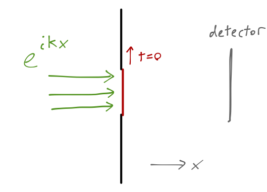
Until t=0, the shutter is closed and the wavefunction remains localized on the left side of the screen (x<0.) At t=0, we open the shutter; what does the profile of the traveling wave look like as time evolves? If we put a detection screen at some distance in front of the shutter, what will we observe?
The propagator makes these questions very straightforward to answer. The initial wavefunction is a plane wave trapped on the left side of the barrier, or \psi(x,0) = \Theta(-x) e^{ikx}. The wavefunction at time t is then just given by integrating this with the free propagator: \psi(x,t) = \int_{-\infty}^\infty dx' K_{\textrm{free}}(x,t; x',0) \psi(x',0) \\ = \sqrt{\frac{m}{2\pi i \hbar t}} \int_{-\infty}^0 dx' \exp \left[ \frac{i}{\hbar} \left( \frac{m (x-x')^2}{2t} + \hbar kx' \right) \right] Since we have an integral from -\infty to 0 and the function isn’t even in x', this is a bit more complicated than just a Gaussian integral, but it’s not too bad; Mathematica or some careful pen-and-paper work will give you the result \psi(x,t \geq 0) = \frac{1}{2} \exp \left( ikx - i k^2 \tau \right) {\rm erfc} \left( \frac{x-k\tau}{\sqrt{2i \tau}} \right) where \tau \equiv \hbar t/m. “Erfc” is the complementary error function, equal to 1 minus the integral of a Gaussian curve; it looks like a smoother version of the Heaviside step function, equal to 1 at large, negative arguments and 0 for large and positive arguments. (It tends to show up in cases like this where we integrate over Gaussian integrands but not over the full range of x.) The total solution is a convolution of this smoothed-out step shape with a plane wave, and looks something like this:
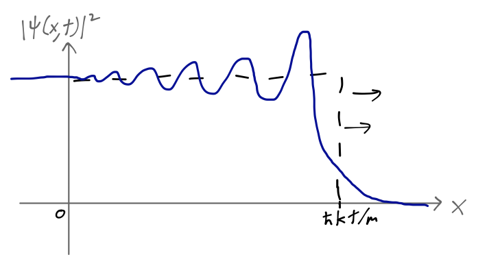
The wavefront here, defined as the point where the error function argument is zero, is at x = k \tau = \hbar k t / m = pt/m, exactly how a classical particle would move. In the classical limit \hbar \rightarrow 0, the error function becomes infinitely steep, and we find a perfectly localized “wavefront”, corresponding to the leading edge of the classical beam.
Quantum mechanically, this edge is smeared out; once we localized the wave at x=0, t=0, the evolution of different momentum components as a wave packet caused some spreading to occur. Still, if we performed the experiment of putting the screen in front of the shutter, we would find roughly zero probability of a particle hitting the screen for t < mx/\hbar k, and roughly unit probability for t > mx/\hbar k.
25.4.3 The double-slit experiment
Another nice application of the free propagator is to one of the first experiments you probably encountered in discussing quantum mechanics, which is the double-slit experiment:
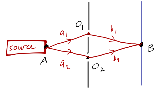
The wavefunction at point B on the screen at time t is given precisely by the propagator from the source at A, \left\langle B, t | A, 0 \right\rangle. We can decompose this propagator into the product of propagators from A to the barrier, and from the barrier to B. However, there are two possible paths now; the particle can either go through the upper opening O_1, or the lower opening O_2. From a probability point of view, these are completely independent events; the particle either goes through O_1 or O_2. Thus, the total probability amplitude can be written as a sum, \left\langle B,t | A,0 \right\rangle = \int_0^t dt_1 \left\langle B,t | O_1,t_1 \right\rangle \left\langle O_1,t_1 | A,0 \right\rangle + \int_0^t dt_2 \left\langle B,t | O_2,t_2 \right\rangle \left\langle O_2,t_2 | A,0 \right\rangle. This may look confusing at first; above, I said there is a spatial integration but no time integration when inserting a complete set of states. But now I’m writing just the opposite! What gives? Both are a result of the specific experimental setup here, in which we’re requiring our particle to propagate through the points O_1 or O_2. The positions of these openings collapse our integral over intermediate position to just the sum over O_1 and O_2 shown above. As for the time integration, that has been added to account for the fact that although our particles must pass through O_1 or O_2, the precise time at which they do so will vary depending on their speed. We could simplify by specifying a perfectly monochromatic source, i.e. fixed momentum, which would then fix t_1 and t_2 and remove the integrals.
Each of the four individual propagators is nothing more than the free-particle propagator, for example \left\langle O_1,t_1 | A,0 \right\rangle = \left( \frac{m}{2\pi i \hbar t_1} \right) \exp \left( \frac{im a_1^2}{2\hbar t_1} \right) where a_1 is the distance from A to O_1 as on the sketch. (This is also written in two dimensions, which changes the normalization factor, but we’re really interested in the phase to study interference effects so this isn’t really important.)
Here, you should complete Tutorial 12 on “Propagators and double-slit interference”. (Tutorials are not included with these lecture notes; if you’re in the class, you will find them on Canvas.)
Much of the detail here is on the tutorial, but if we plot the real part of the phase of \left\langle B,t | O_1,t_1 \right\rangle \left\langle O_1,t_1 | A,0 \right\rangle, we notice that as a function of the form e^{ix^2}, it looks something like this:
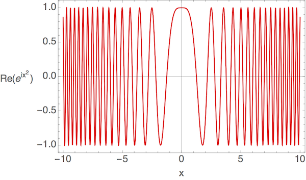
As done in the tutorial exercise, this sort of function invites the use of stationary-phase approximation, which approximates the result using the dominant contribution near x=0; the rest of the integrand contains rapid oscillating terms that give zero contribution on average. The physical argument for stationary phase is nothing more than the observation that there is a certain time t_1 at which a classical particle with a given speed will tend to hit the screen, and the contribution from other times is much smaller.
Taking approximations like the above in the appropriate way, for all four lengths a_i and b_i approximately equal (but not exactly equal) we find that the squared propagator takes on the familiar form of an interference pattern, |\left\langle B,t | A,0 \right\rangle|^2 \propto 1 + \cos \left( \frac{m (\ell_1 - \ell_2) (\ell_1 + \ell_2)}{2\hbar t} \right) \sim \cos^2 \left( \frac{m (\ell_1 - \ell_2) (\ell_1 + \ell_2)}{4\hbar t} \right). where \ell_i = a_i + b_i is the total path length through each of the two slits.
Notice that the 1/t may look funny, but remember that this is the propagator, which is only equal to the wavefunction if our initial state is really \ket{A,0}, i.e. a sharp delta function localized at the source at time t=0. In this case, we expect non-trivial time dependence. If we have a steady-state source, we would remove t by identifying it as the time of flight from the source, t = \frac{\ell}{v} = \frac{m\ell}{p} = \frac{m\ell}{\hbar k} where \ell = (\ell_1 + \ell_2) / 2, so |\left\langle B,t | A,0 \right\rangle|^2 \sim \cos^2 \left( \frac{k}{2} (\ell_1 - \ell_2) \right) = \cos^2 \left( \frac{\pi (\ell_1 - \ell_2)}{\lambda} \right), matching the textbook result based on wave interference.
25.5 Path integration
We could at this point imagine generalizing this approach to deal with more complicated variants of the same problem. For example, if we had a barrier with three holes, or four, or N we could still find the final interference pattern just by summing over the possible propagator combinations: \left\langle B,t | A,0 \right\rangle = \sum_{i=1}^N \int_0^t dt_i \left\langle B,t | O_i,t_i \right\rangle\left\langle O_i,t_i | A,0 \right\rangle.
25.5.1 A thought experiment: removing the screen
As this thought experiment becomes more complicated, it starts to lead us in an interesting direction. What if we added a second barrier in between the first and the detector?
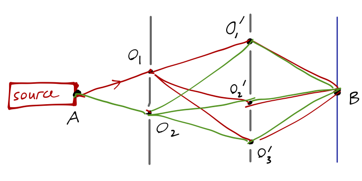
The events of the particle passing through any hole in any barrier are still all independent, so we can write the overall amplitude as a more complicated sum, decomposing into propagators from A to O_i to O'_j to B. While the sum has more terms, the basic idea is the same: the amplitude to travel any one path is just the product of the propagators along each piece of the path. At this point, it’s easy to imagine adding more barriers and more holes; the sum gets more complicated, but the basic principle remains the same - just sum over the propagator products for all possible paths from A to B.
Now here is the important realization: if we take the limit where the number of holes in the barrier goes to infinity, so that there really isn’t any barrier at all, then we’re left with nothing but a particle propagating through empty space! But as we take the limit, we’re still carefully summing over all of the number of possible paths, now approaching infinity. So screens or not, the probability amplitude for a particle to propagate from x to y in time T is equal to the sum over all possible paths from x to y. This was Richard Feynman’s key insight into a new way of formulating quantum mechanics.
Let’s go back to our rigorous definitions now. How do we formally describe such a “sum over paths”? Let’s start by considering the interval from some initial time t_1 to final time t_N, which we’ll subdivide into N-1 equal steps in between: t_j - t_{j-1} = \frac{t_N - t_1}{N-1}. We’ll also call the initial position x_1 and the final position x_N. With no screens in the middle, we want to continuously average over the paths, so the sums become integrals: \left\langle x_N, t_N | x_1, t_1 \right\rangle = \int dx_{N-1} \int dx_{N-2} ... \int dx_2 \\ \hspace{40mm} \left\langle x_N, t_N | x_{N-1}, t_{N-1} \right\rangle \left\langle x_{N-1}, t_{N-1} | x_{N-2}, t_{N-2} \right\rangle ... \left\langle x_2, t_2 | x_1, t_1 \right\rangle. (If you like, this is sort of equivalent to the limit where we still have N screens, but each screen has an infinite number of holes so there is no screen left.) You’ll immediately recognize this as just the application of the composition of propagators, as we defined above. In fact, we could have skipped the digression and just gone right to this equation, as Sakurai does. But I wanted to make the “sum over paths” idea a bit more clear. You should also suspect that this will be a particularly useful way to think about the case where \hat{H} depends explicitly on time (imagine a different \hat{H} appearing in each of the infinitesimal propagators.)
25.5.2 The path integral
Now we’re ready to return to the quantum expression for the propagator. Notice that we can rewrite each of the intermediate propagators by pulling out the time evolution to find \left\langle x_j, t_j | x_{j-1}, t_{j-1} \right\rangle = \bra{x_j} \exp \left( - \frac{i\hat{H} \Delta t}{\hbar} \right) \ket{x_{j-1}}. Since we’re studying the evolution of a single particle, let’s split the Hamiltonian up into the kinetic and potential energy terms, \hat{H} = \frac{\hat{p}^2}{2m} + V(\hat{x}). Since \hat{x} and \hat{p} don’t commute, normally we wouldn’t be able to split up the exponential. But since we’re dealing with the infinitesimal time-step \Delta t, we can rewrite \exp \left( -\frac{i\hat{H} \Delta t}{\hbar} \right) = \exp \left( -\frac{i \hat{p}^2 \Delta t}{2m \hbar} \right) \exp \left( -\frac{i V(\hat{x}) \Delta t}{\hbar} \right) + \mathcal{O}(\Delta t^2). Inserting a complete set of states then gives \left\langle x_j, t_j | x_{j-1}, t_{j-1} \right\rangle = \int dx' \bra{x_j} \exp \left( -\frac{i \hat{p}^2 \Delta t}{2m\hbar} \right) \ket{x'} \bra{x'} \exp \left( -\frac{i V(\hat{x}) \Delta t}{\hbar} \right) \ket{x_{j-1}} \\ = \int dx' \bra{x_j} \exp \left( -\frac{i \hat{p}^2 \Delta t}{2m\hbar} \right) \ket{x'} \exp \left( -\frac{i V(x_{j-1}) \Delta t}{\hbar} \right) \delta(x' - x_{j-1}). The first expression is just the free-particle propagator which we’re now familiar with, and the delta function from the second term collapses the integral, so we have \left\langle x_j, t_j | x_{j-1}, t_{j-1} \right\rangle = \sqrt{\frac{m}{2\pi i \hbar \Delta t}} \exp \left[ \left( \frac{m(x_j - x_{j-1})^2}{2 (\Delta t)^2} - V(x_{j-1}) \right) \frac{i \Delta t}{\hbar} \right].
(As a very brief aside, this equation has exactly the sort of form that would be useful for setting up numerical solutions of quantum time evolution in the usual way, by evaluating finite differences repeatedly.) Plugging back in to the full propagator above, we thus find \left\langle x_N, t_N | x_1, t_1 \right\rangle = \left( \frac{m}{2\pi i \hbar \Delta t}\right)^{(N-1)/2} \int dx_{N-1} dx_{N-2} ... dx_2 \\ \exp \left[ \frac{i \Delta t}{\hbar} \sum_{j=2}^{N-1} \left(\frac{1}{2} m \left( \frac{x_{j+1} - x_j}{\Delta t}\right)^2 - V(x_j) \right) \right] Finally taking the limit \Delta t \rightarrow 0, the difference becomes a derivative and the sum an integral:
The formal solution to the propagator for a general quantum system can be written in terms of the Feynman path integral,
\lim_{\Delta t \rightarrow 0} \left\langle x_N, t_N | x_1, t_1 \right\rangle = \int \mathcal{D}[x(t)] \exp \left[ \frac{i}{\hbar} \int_{t_1}^{t_N} dt \left( \frac{1}{2} m \dot{x}(t)^2 - V(x(t)) \right) \right]. \\ = \int_{x_1}^{x_N} \mathcal{D}[x(t)] \exp \left[ \frac{i}{\hbar} \int_{t_1}^{t_N} dt\ \mathcal{L}(x, \dot{x}) \right] \\ = \int_{x_1}^{x_N} \mathcal{D}[x(t)] \exp \left[ \frac{iS(x,\dot{x})}{\hbar} \right]. The script D denotes the “path integration” itself, which is the properly-normalized infinite-dimensional limit of our interval subdivision, \int_{x_1}^{x_N} \mathcal{D}[x(t)] \equiv \lim_{N \rightarrow \infty} \left( \frac{m}{2\pi i \hbar \Delta t} \right)^{(N-1)/2} \int dx_{N-1} \int dx_{N-2} ... \int dx_2. The quantity S = \int dt\ \mathcal{L} is the action, the same function which appears mysteriously in the derivation of the Lagrangian framework in classical mechanics.
Path integrals are a radically different-looking way to formulate quantum mechanics, but one which is equivalent to the Schrödinger approach we’ve been working in. In fact, it’s straightforward to go in the opposite direction: start with the path integral and derive the time-dependent Schrödinger equation.
We can even solve for the dynamics of quantum systems using the path integral, at least in principle. As Sakurai points out, the path integral can be exactly evaluated for the simple harmonic oscillator, giving the propagator (and with a little more work, the energy eigenfunctions and corresponding energy levels.) Unfortunately, the path integral is intractable for all but the simplest non-relativistic quantum systems. Our goal will mostly be to use it as a formal construct, to give us useful insights into gauge symmetry that are much more obscure without the path integral.
In quantum field theory and statistical mechanics, the path integral sees much more practical use. In fact, there is a subfield known as lattice field theory which turns the infinite-dimensional path integral into a finite-dimensional object by discretizing space and time into a finite lattice, and then uses Monte Carlo methods to evaluate the path integral numerically. But that’s a story for another class!
25.5.3 WKB and path integration
The path integral provides us with a very intuitive way of seeing how classical mechanics arises from quantum mechanics, and in particular why a classical system should satisfy the principle of least action. Suppose we want to compare the contribution of two paths to the overall propagator, one with action S_0, and another with action S_0 + \delta S. As we’ve seen, the total contribution is the sum over the paths of e^{iS/\hbar}, i.e. \exp \frac{i S_0}{\hbar} + \exp \left(\frac{i (S_0 + \delta S)}{\hbar} \right) = e^{iS_0 / \hbar} \left(1 + e^{i \delta S / \hbar} \right). If we average over many paths, “integrating” over \delta S in the formal sense, we see that if the changes in action are large compared to \hbar, then the phase will oscillate wildly; as the phase varies, it will go from 1 to -1 and anywhere in between in the complex plane, and we can find large cancellations. The only sets of paths which will contribute significantly, similar to what we saw in the two-slit example above, are those which add coherently, i.e. for which \delta S \approx 0. Turning points of the action, where \delta S changes slowly as the path is deformed, are exactly those paths given by the Euler-Lagrange equations; they are the classical paths.
We can make this idea more concrete by connecting back to the other way we had of trying to obtain a semi-classical limit, which was the WKB approximation. To make this connection, our starting point is the path-integral expression for the propagator, K(x',t';x, t) = \int_{x}^{x'} \mathcal{D}[x(t)] \exp \left[ \frac{i}{\hbar} \int_{t}^{t'} dt\ \mathcal{L}(x,\dot{x}) \right]. As we know, the classical solution for the motion in a given system corresponds to a turning point of the action S = \int dt\ \mathcal{L}; the contributions of paths near the classical path constructively interfere.
This means that the path integral will be dominated by paths close to the classical solution x_{\rm cl}. We can expand x = x_{\rm cl} + y, and then rewrite as an integration over the small differences y = x - x_{\rm cl} to the classical trajectory, K = \int \mathcal{D}[y] \exp \left[ \frac{i}{\hbar} \int_{t}^{t'} dt\ \mathcal{L}(x_{\rm cl} + y, \dot{x}_{\rm cl} + \dot{y}) \right] This can be expanded out in terms of variations of the action \delta S, but rather than getting too far into the details, we’ll just work with the leading-order approximation, which is that the lowest-order result of the integration is just using the classical path: K(x',t'; x, t) \approx C \exp \left[ \frac{i}{\hbar} \int_t^{t'} dt\ \mathcal{L}(x_{\rm cl}, \dot{x}_{\rm cl}) \right]. We’re working with Schrödinger’s equation in an arbitrary potential, which means we’ve explicitly assumed the form of the Lagrangian is \mathcal{L}(x, \dot{x}) = \frac{1}{2} m \dot{x}^2 - V(x). Now, for the WKB approximation we are working with energy eigenstate solutions \psi_E(x), which means we’ve separated out the time dependence from the spatial dependence in the wavefunction. To make this more explicit in the current approach, we assume our classical solution corresponds to total energy E. We know the relationship between the classical solution and the energy: E = \frac{1}{2}m \dot{x}_{\rm cl}^2 + V(x_{\rm cl}), which lets us eliminate the potential in favor of the energy: K(x',t'; x,t) \approx C \exp \left[ \frac{i}{\hbar} \int_{t}^{t'} dt\ \left( m \dot{x}_{\rm cl}^2 - E \right) \right] \\ = C \exp \left[ \frac{im}{\hbar} \int_{t}^{t'} dt\ \dot{x}_{\rm cl}^2 \right] \exp \left[ \frac{-iE (t'-t)}{\hbar} \right], splitting the time-dependence out in the expected form. Focusing on the remaining part, since we know what we’re working towards, let’s rewrite one of the two velocity terms using p \equiv m \dot{x}_{\rm cl}. Using the other to swap limits of integration, K(x',t'; x,t) \approx C \exp \left[ \frac{i}{\hbar} \int_x^{x'} dx\ p(x) \right] \exp \left[ \frac{-iE (t'-t)}{\hbar} \right]. Since the temporal and spatial parts are fully separated, we can read off the evolution for the spatial wavefunction from the first part: recalling that \psi(x',t') = \int dx'' K(x', t'; x'',t) \psi(x'',t) we can just insert a delta function for the initial spatial wavefunction to obtain \psi(x',t') \sim C \exp \left[ \frac{-iEt'}{\hbar} \right] \exp \left[ \frac{i}{\hbar} \int_x^{x'} dx\ p(x) \right].
This more or less recovers our WKB wavefunction, except that we’re missing the 1/\sqrt{k(x)} that came from the next-to-leading order term in the \hbar expansion. This is exactly what we’ve discarded by just keeping the classical action; if we go back and carefully do the path integral over the path variations y(t), we will find a Gaussian integral that we can evaluate to get the 1/\sqrt{k} and recover the WKB approximation in full. So we see that making the idea of just keeping small fluctuations around the classical path concrete leads to exactly the WKB approximation - two equivalent ways of thinking about a semi-classical limit!