4 Time evolution in quantum mechanics
So far, we’ve set up a lot of formalism to discuss static properties of a quantum system. But there is a lot more interesting physics in the dynamics of a quantum system - that is, in describing how it evolves in time. From postulate 5, time evolution of quantum states is governed by the Schrödinger equation, i\hbar \frac{\partial}{\partial t} \ket{\psi(t)} = \hat{H} \ket{\psi(t)}.
To understand what this means and how to use it, we have to define the Hamiltonian operator, \hat{H}, which appears in the equation. As the name suggests, \hat{H} is exactly the quantum analogue of the Hamiltonian as defined in classical mechanics. (In fact, you may have seen discussions where some classical H is “quantized” to produce the quantum \hat{H} - but of course, quantum mechanics is the more fundamental theory, so really this is going backwards!)
We can get a bit of intuition by thinking about dimensions in the Schrödinger equation. The constant \hbar, Planck’s constant, has units of energy times time: I’ve referred to it before, but now that we’re thinking about units I’ll remind you of its value:
Planck’s constant \hbar is equal to, in SI units and also in more convenient units for atomic physics,
\hbar \approx 1.05 \times 10^{-34}\ {\rm J} \cdot {\rm s} \approx 6.58 \times 10^{-16}\ {\rm eV} \cdot {\rm s}.
For historical reasons, \hbar is really called the “reduced Planck’s constant”, while “Planck’s constant” is reserved for h = 2\pi \hbar. But in quantum mechanics, \hbar is the thing which appears more often, so I’ll always work with \hbar instead of h and will usually just call \hbar “Planck’s constant”.
By inspection, then, the quantum Hamiltonian \hat{H} has to have units of energy. In fact, in a typical quantum system \hat{H} is an observable, corresponding to the total energy of our quantum system. (Again, this is in direct analogy to classical mechanics, where in most systems H corresponds to the total energy E.) This means that the eigenstate of \hat{H} are energy eigenstates, state with definite energy: \hat{H} \ket{E} = E \ket{E}.
Now, if \hat{H} is an observable then it has to be Hermitian. Let’s suppose that \hat{H} is time-independent, \partial \hat{H} / \partial t = 0. (This clearly corresponds to the total energy of the system being conserved, dE/dt = 0; we’ll deal with time-dependent Hamiltonians later.) Then we can formally integrate the Schrödinger equation to find the solution \ket{\psi(t)} = \exp\left[ \frac{-i}{\hbar} \hat{H} t \right] \ket{\psi(0)} \equiv \hat{U}(t) \ket{\psi(0)}. If \hat{H} is Hermitian, then the operator \hat{U}(t) which evolves our state in time is unitary. Recall that our probabilistic interpretation of physical states requires them to have norm 1; as long as time evolution is unitary, these states will always have norm 1. We say that a theory with a unitary time evolution has conservation of probability. This also tells us that the only systems where \hat{H} is not an observable giving the total energy are ones where probability is not conserved - typically “open” systems which have some interaction with an external environment.
From here forward, we’ll always assume \hat{H} is Hermitian unless explicitly noted otherwise. We can then see that the bras evolve in time according to the adjoint equation -i\hbar \frac{\partial}{\partial t} \bra{\psi(t)} = \bra{\psi(t)} \hat{H}{}^\dagger = \bra{\psi(t)} \hat{H} as long as \hat{H} is Hermitian; if it’s also time-independent we can write down a formal solution again, just with an extra minus sign, \bra{\psi(t)} = \bra{\psi(0)} \exp \left[ \frac{+i}{\hbar} \hat{H} t \right] = \bra{\psi(0)} \hat{U}^\dagger(t).
4.0.1 Solving for time evolution
Let’s turn from formalism to practical thoughts. Although the formal solutions to the Schrödinger equation above are correct, for most problems they’re also not particularly useful. In order to apply them, we have to calculate the exponential of \hat{H}. It is true that the exponential of an operator can be written in general as a power series, \exp(\hat{A}) \equiv \sum_{k=0}^\infty \frac{1}{k!} \hat{A}{}^k. This allows us to write out the time evolution operator as \exp \left[ \frac{-i}{\hbar} \hat{H} t \right] = \hat{1} - \frac{i}{\hbar} t \hat{H} - \frac{1}{2\hbar^2} t^2 \hat{H}{}^2 + ... Unfortunately, for a generic \hat{H} we can’t write the answer in closed form; we need to compute every power of \hat{H}. The only exception is when the series terminates, i.e. when some power of \hat{H} gives us 1 or 0 and the sequence starts to repeat; or when some part of \hat{H} t is so small that we can truncate the series and ignore the higher terms.
Fortunately for us, there is another approach that we can always use. If we expand our arbitrary state \ket{\psi} in the energy eigenstates, then \ket{\psi(t)} = \sum_E \exp \left[ -\frac{i}{\hbar} \hat{H} t \right] \ket{E} \left\langle E | \psi(0) \right\rangle \\ \Rightarrow \left\langle E | \psi(t) \right\rangle = \left\langle E | \psi(0) \right\rangle e^{-iEt/\hbar}. In other words, if we expand our initial state \ket{\psi(t_0)} in energy eigenstates, then the coefficients of the expansion evolve simply in time by picking up an oscillating phase determined by the energy eigenvalue.
Notice that the probability of observing energy E_j at any time is p(E_j) = |\left\langle E_j | \psi(t) \right\rangle|^2 = |\left\langle E_j | \psi(0) \right\rangle|^2 which is time-independent. However, this is special to energy: eigenstates of some other observable \hat{A} will generally become mixtures of eigenstates as the system evolves. The exception is when \hat{A} commutes with the Hamiltonian, [\hat{A}, \hat{H}] = 0. As you know, this means that we can find a common set of eigenvectors for \hat{A} and \hat{H}, and thus if \ket{\psi(t_0)} = \ket{a, E_a}, then \ket{\psi(t)} = \ket{a, E_a} \exp \left(-\frac{i E_a t}{\hbar}\right). In other words, the system remains in an eigenstate \ket{a, E_a} of \hat{A} with eigenvalue a (and energy E_a) for all time. The state isn’t completely identical; it picks up a complex phase factor. But there’s no mixing of eigenstates as the system evolves. As you might guess, finding observables that commute with \hat{H} is a very important task in dynamical quantum mechanics!
4.1 Example: Larmor precession
Now that we understand the energy eigenstates in the generalized two-state system, let’s see what happens to it under time evolution. We’ll consider the specific example of an electron in an external magnetic field, which has the following Hamiltonian: \hat{H} = -\hat{\vec{\mu}} \cdot \vec{B} = \frac{e}{mc} \hat{\vec{S}} \cdot \vec{B}. As the hats remind us, the magnetic field is a classical field which exists in the background, so it’s not an operator, just an ordinary vector. In fact, in the usual \hat{S_z} basis we know that the spin operators are proportional to the Pauli matrices \vec{\sigma}, and so we can expand out the dot product as \hat{\vec{S}} \cdot \vec{B} = \frac{\hbar}{2} \hat{\vec{\sigma}} \cdot \vec{B} = \frac{\hbar}{2} \left( \begin{array}{cc} B_z & B_x - iB_y \\ B_x + iB_y & -B_z \end{array} \right). It’s convenient to define the quantity \omega = \frac{e|B|}{mc} in which case we simply have \hat{H} = \frac{\hbar \omega}{2} (\hat{\vec{\sigma}} \cdot \vec{n}), where \vec{n} is a unit vector pointing in the direction of the applied magnetic field. The angular frequency \omega is known as the Larmor frequency.
A word of warning: I’m following Sakurai and using “Gaussian” or “cgs” units, which includes some extra factors of c in the definitions of electromagnetic fields. See appendix A of Sakurai for how to convert between Gaussian and SI units. If you try to plug in an SI magnetic field above you will get a wave number and not a frequency, so at least you’ll know something is wrong!
In general, the Hamiltonian will not commute with any of the spin operators, since it is a combination of all three. However, since we’re studying the spin-1/2 system in complete isolation, there’s nothing stopping us from calling the magnetic field direction z. Then we can see that [\hat{H}, \hat{S_z}] = 0, and our Hamiltonian becomes \hat{H} = \frac{\hbar \omega}{2} \left( \begin{array}{cc} 1 & 0 \\ 0 & -1 \end{array} \right) which is already diagonal, with eigenvalues E_{\pm} = \pm \hbar \omega/2. Because it is already diagonal, we can find the time evolution of an arbitrary state in a very simple way by expanding in \hat{S}_z eigenstates. For example, given an arbitrary initial state \ket{\psi(0)} = \alpha \ket{\uparrow} + \beta \ket{\downarrow}, the time-evolution operator \hat{U}(t) just acts on each of the basis states according to its eigenvalue, so we have simply \ket{\psi(t)} = \hat{U}(t) \ket{\psi(0)} \\ = e^{-i\hat{H} t/\hbar} (\alpha \ket{\uparrow} + \beta \ket{\downarrow}) \\ = \alpha e^{-i\omega t/2} \ket{\uparrow} + \beta e^{+i\omega t/2} \ket{\downarrow}.
Notice that if we compute the probability of measuring \hat{S}_z = +\hbar/2 as a function of time, we find that it is time-independent: p(S_z = +) = |\left\langle \uparrow | \psi(t) \right\rangle|^2 = \left| \bra{\uparrow} (\alpha e^{-i\omega t/2} \ket{\uparrow} + \beta e^{+i\omega t/ 2} \ket{\downarrow}) \right|^2 \\ = |\alpha|^2 |\bra{\uparrow} e^{-i\omega t/2} \ket{\uparrow}|^2 = |\alpha|^2 for any t. (This might be a little surprising, but it makes sense; \hat{S}_z is proportional to the Hamiltonian so this is just an energy measurement, and the lack of time evolution in this quantity is basically just energy conservation!)
Here, you should complete Tutorial 2 on “Larmor precession”. (Tutorials are not included with these lecture notes; if you’re in the class, you will find them on Canvas.)
On the tutorial, you studied the evolution of the initial state \ket{\psi(0)} = \frac{1}{\sqrt{2}} (\ket{\uparrow} + \ket{\downarrow}), which is the spin-up eigenket in the x direction. The quantum evolution gives us a rather simple result for the expectation values: \left\langle \hat{S_x} \right\rangle = \frac{\hbar}{2} \cos \omega t, \left\langle \hat{S_y} \right\rangle = \frac{\hbar}{2} \sin \omega t, \\ \left\langle \hat{S_z} \right\rangle = 0. The applied z-direction magnetic field causes the spin to rotate, or precess, in the xy plane; this particular example is known as Larmor precession. This is a very important effect; I’ve glossed over the point that the Larmor precession frequency is more generally defined as \omega = \frac{eg|B|}{2mc}, where the quantity g is an intrinsic property of the charged object, relating angular momentum to the magnetic moment. For a classical spinning charged sphere, g=1; for the electron, quantum effects lead to g=2.
In fact, g is not exactly two for the electron; quantum electrodynamics, the quantum field theory which describes the electromagnetic force, predicts small corrections as a power series in the fine-structure constant \alpha \approx 1/137. Experiments to measure the Larmor precession of electrons and theoretical calculations of this power series have been carried out to extraordinary precision, and the agreement between the two is now at a level below 1 part per trillion.
4.1.1 Application: muon (g-2)
We’ve been doing a lot of theory, so let’s talk briefly about experimental determination of the muon (g-2). (This is a more direct application of what we’ve just done than electron (g-2) experiments, which tend to exploit atomic physics.) The Larmor frequency \omega looks a lot like a familiar classical expression, which is the cyclotron frequency: a classical charge of magnitude e will undergo circular motion in a transverse magnetic field with angular frequency
\omega_c = \frac{e|B|}{mc}
This suggests a straightforward way to set up an experiment: we inject a beam of muons into a circular storage ring with magnetic field applied in the \hat{z} direction. The muon is unstable and will decay into an electron (plus neutrinos), and the direction of the outgoing electron turns out to be correlated with the direction of the muon’s spin, so we can measure the spin direction by looking for electrons coming out.
Now, if g is exactly 2 for the muon, then if we put a detector at a fixed point on our storage ring, the spin will precess at precisely the same rate as the motion around the ring, which means that we should never see any variation in the muon’s spin direction. If there is an anomalous contribution to (g-2), then we’ll see it as a modulated signal, i.e. we expect an anomalous precession frequency
\omega_a = \frac{(g-2)e|B|}{2mc}.
Here’s what the ongoing Muon (g-2) Experiment at Fermi National Laboratory has seen recently:
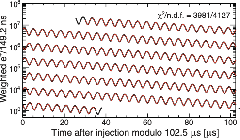
This is a really beautiful plot: there is no manipulation for presentation, this is raw experimental data (and a fit). Muons decay into electrons, so the number of counts dies off exponentially over time as shown. By eye, the oscillation period is about 5 microseconds, which translates to (g-2)/2 \sim 0.001. Of course, this is just a summary plot, the real experimental measurement is much more precise: the present world average (dominated by the latest Fermilab measurements) is
\frac{g_\mu - 2}{2} = 0.001165920715(145).
I’ve ignored all kinds of important details here, of course, not least of which is relativistic effects since the muons have to be moving pretty fast to make the experiment work! But the basic idea here is very simple. The experiment itself is a masterful piece of precision physics, and if you’re interested I invite you to look at their recent paper to see all the details.
The Standard Model of particle physics predicts a value of the muon (g-2) which is very close to the number given above, but depending on the method used there is some tension. More work is needed on the theory side (which I am involved in!) to finish the story here. If the theory prediction agrees precisely, this is a very powerful constraint on possible models of new physics.
4.1.2 Arbitrary magnetic field directions
The previous example exploited the fact that time evolution acts simply on eigenstates of the Hamiltonian, which were also eigenstates of the \hat{S}_z operator. However, more generally we might be interested in the case where the Hamiltonian is not simply proportional to \hat{S}_z. If we allow the magnetic field to point in any direction, then we find the Hamiltonian \hat{H} = \frac{\hbar \omega}{2} \hat{\vec{\sigma}} \cdot \vec{n}, where \vec{n} = \vec{B} / |\vec{B}| is a unit vector in the direction of the applied magnetic field. (If this is the entire Hamiltonian, then we’re just making life harder for ourselves by not rotating our coordinates to make \vec{n} = \hat{z}! But there are plenty of systems that have this interaction as one of many.)
For this case, it can be helpful to just use exponentiation directly; you’ve tried this on the homework for a simpler case. Recall that earlier we wrote down a formal expression for the time-evolution operator when \hat{H} itself is time-independent, namely \hat{U}(t) = e^{-i\hat{H} t/\hbar} = e^{-i \omega t \hat{\vec{\sigma}} \cdot \vec{n}/2}. We know that this exponential can be rewritten as a power series, e^{-i\omega t \hat{\vec{\sigma}} \cdot \vec{n}/2} = \hat{1} - \frac{i \omega t}{2} (\hat{\vec{\sigma}} \cdot \vec{n}) + \frac{1}{2} \left(\frac{i \omega t}{2}\right)^2 (\hat{\vec{\sigma}} \cdot \vec{n})^2 + ... Taking powers of (\hat{\vec{\sigma}} \cdot \vec{n}) isn’t as easy as it looks, since we know the three Pauli matrices don’t commute with each other. However, we can show that the product of two Pauli matrices satisfies the identity \hat{\sigma}_i \hat{\sigma}_j = i \epsilon_{ijk} \hat{\sigma}_k + \hat{1} \delta_{ij}, and thus (\hat{\vec{\sigma}} \cdot \vec{n})^2 = \hat{\sigma}_i n_i \hat{\sigma}_j n_j \\ = \left( i \epsilon_{ijk} \hat{\sigma}_k + \hat{1} \delta_{ij} \right) n_i n_j. (Note that here I am using the Einstein summation convention, that when you see repeated indices they are implicitly summed over. If it’s ever unclear in a particular situation I will write explicit sums.)
Anyway, since \vec{n} is a unit vector pointing in some direction, we know that \epsilon_{ijk} n_i n_j = \vec{n} \times \vec{n} = 0, and \delta_{ij} n_i n_j = \vec{n} \cdot \vec{n} = 1. So (\hat{\vec{\sigma}} \cdot \vec{n})^2 = \hat{1}, which means that (\hat{\vec{\sigma}} \cdot \vec{n})^3 = \hat{\vec{\sigma}} \cdot \vec{n}, and so forth. This immediately lets us write our infinite sum of matrix products as a pair of infinite sums multiplied by known matrices: e^{-i\omega t \hat{\vec{\sigma}} \cdot \vec{n}/2} = \sum_{k=0}^\infty \frac{1}{k!} \left[ \left(\frac{i \omega t}{2}\right) \hat{\vec{\sigma}} \cdot \vec{n}\right]^k \\ = \sum_{k=0}^\infty \left[ \frac{1}{(2k)!} (i \omega t)^{2k} \hat{1} + \frac{1}{(2k+1)!} (i \omega t)^{2k+1} (\hat{\vec{\sigma}} \cdot \vec{n}) \right] \\ = \hat{1} \cos \frac{\omega t}{2} - i (\hat{\vec{\sigma}} \cdot \vec{n}) \sin \frac{\omega t}{2}. Writing it out in matrix form, \hat{U}(t) = \left( \begin{array}{cc} \cos \omega t/2 - i n_z \sin \omega t/2 & (-i n_x - n_y) \sin \omega t/2 \\ (-i n_x + n_y) \sin \omega t/2 & \cos \omega t/2 + i n_z \sin \omega t/2 \end{array} \right). I leave it as an exercise to verify that this is (as expected) a unitary matrix, i.e. \hat{U}{}^\dagger \hat{U} = \hat{1}, and that setting n_z = 1 recovers the time evolution we found in the Larmor precession example.
It can be instructive to see another way to calculate the same matrix, which is easier to work with in cases where summing the power series as we did above is hard. This is basically what we did for Larmor precession - using expansion in energy eigenstates - but in this case we don’t have a simple basis in which \hat{H} is diagonal.
Remember that we can rewrite the time evolution operator by summing over energy eigenstates, \hat{U}(t) = e^{- i\hat{H}t / \hbar} = \sum_{i} \sum_j \ket{E_i} \bra{E_i} e^{-i\hat{H} t/\hbar} \ket{E_j} \bra{E_j} \\ = \sum_i \ket{E_i} e^{-i \hat{E_i} t/\hbar} \bra{E_i}. So to find the evolution operator, we just need to compute the eigenvalues and eigenvectors of \hat{H}, which in matrix form looks like \hat{H} = \frac{\hbar \omega}{2} \left( \begin{array}{cc} n_z & n_x - in_y \\ n_x + in_y & -n_z \end{array} \right). We diagonalized this matrix last time; here we identify the energy splitting \epsilon = \hbar \omega n_z/2 and the off-diagonal term \delta = \hbar \omega (n_x - in_y) / 2. The average energy is 0, so that the energy eigenvalues are E_{\pm} = \pm \sqrt{\epsilon^2 + |\delta|^2} = \pm \sqrt{ (\hbar \omega / 2)^2} \sqrt{n_z^2 + n_x^2 + n_y^2} = \pm \hbar \omega/2. The mixing angle which determines the eigenstates is \tan 2\alpha = \frac{\epsilon}{|\delta|} = \frac{n_z}{\sqrt{n_x^2 + n_y^2}} and the phase \phi is given by the expression e^{i\phi} = \frac{\delta^\star}{|\delta|} = \frac{n_x + in_y}{\sqrt{n_x^2 + n_y^2}} These are, in fact, exactly the spherical angles defining the unit vector \vec{n} itself! The only oddity is that the mixing angle \alpha is half of the coordinate-space angle \theta. So the eigenstates are, referring back to our previous work, \ket{\uparrow} = \left( \begin{array}{c} \cos (\theta/2) \\ \sin (\theta/2) e^{i \phi} \end{array} \right) \\ \ket{\downarrow} = \left( \begin{array}{c} -\sin (\theta/2) \\ \cos (\theta/2) e^{i \phi} \end{array} \right) giving the outer products \hat{U}(t) = e^{-i \omega t/ 2} \ket{\uparrow} \bra{\uparrow} + e^{i \omega t /2} \ket{\downarrow} \bra{\downarrow} \\ = \left( \begin{array}{cc} \cos^2 (\theta/2) e^{-i\omega t/2} + \sin^2 (\theta/2) e^{i \omega t/2} & \cos (\theta/2) \sin (\theta/2) e^{-i\phi} (e^{-i \omega t/2} - e^{i \omega t /2}) \\ \cos (\theta/2) \sin (\theta/2) e^{i\phi} (e^{-i \omega t/2} - e^{i \omega t/2}) & \sin^2 (\theta/2) e^{-i\omega t/2} + \cos^2 (\theta/2) e^{i \omega t/2} \end{array} \right) \\ = \left( \begin{array}{cc} \cos (\omega t/2) - i \cos \theta \sin (\omega t/2) & -i\sin (\omega t/2) \sin \theta e^{-i \phi} \\ -i\sin(\omega t/2) \sin \theta e^{i\phi} & \cos (\omega t /2) + i \cos \theta \sin(\omega t/2) \end{array} \right) recovering our result above, in a slightly different notation.
4.2 Example: magnetic resonance
As a lead-in to our next topic, let’s look at another situation which is very hard to deal with in general, but tractable for the two-state system; explicit time variation in the Hamiltonian. The physical effect that we will be studying here is known as magnetic resonance, and is one of the more important applications of the two-state system.
(Note: beware factors of 2 in the definitions of frequencies if you look up this derivation elsewhere!)
Let’s apply an external magnetic field which has a large, constant component B in the z direction, and a small component which rotates around the xy plane with angular frequency \nu: \vec{B} = (b \cos \nu t, b \sin \nu t, B). This is just a specific choice of an external magnetic field, so we can write the Hamiltonian like we did in the previous example, \hat{H} = \frac{\hbar \omega}{2} \hat{\sigma}_z + \frac{\hbar \Omega_0}{2} \left( \hat{\sigma}_x \cos (\nu t) + \hat{\sigma}_y \sin (\nu t) \right) = \frac{\hbar}{2} \left( \begin{array}{cc} \omega & \Omega_0 e^{-i\nu t} \\ \Omega_0 e^{i \nu t} & -\omega \end{array} \right) where we’ve now defined two angular frequencies \omega = \frac{eB}{mc}, \\ \Omega_0 = \frac{eb}{mc}. This time, we’ll apply the Schrödinger equation directly; since this is a two-state system, we end up with a pair of coupled differential equations. If we define \ket{\psi(t)} = \left( \begin{array}{c} a_+(t) \\ a_-(t) \end{array} \right) then applying the Hamiltonian, we find i \hbar \frac{d}{dt} \ket{\psi(t)} = \hat{H} \ket{\psi(t)} \\ \begin{cases} 2i \dot{a}_+ &= \omega a_+ + \Omega_0 e^{-i\nu t} a_- \\ 2i \dot{a}_- &= \Omega_0 e^{i\nu t} a_+ - \omega a_-. \end{cases} where I’m using the common shorthand notation \dot{a}_{\pm} = da_{\pm}/dt. We can solve this coupled system by ansatz (physics jargon for a clever guess). Noticing the complex exponential time dependence, if we assume the same is true for the wavefunction solution, i.e. a_{\pm} = A_{\pm} e^{-i \lambda_{\pm} t}, then in matrix form, we arrive at the equation \left( \begin{array}{cc} 2\lambda_+ - \omega & -\Omega_0 e^{-i(\nu -\lambda_+ + \lambda_-)t} \\ -\Omega_0 e^{i(\nu - \lambda_+ + \lambda_-)t} & 2 \lambda_- + \omega \end{array} \right) \left( \begin{array}{c} A_+ \\ A_- \end{array} \right) = 0. Now we see that the time dependence is entirely removed if we choose \lambda_+ = \lambda_- + \nu. That just leaves us with the simple system \left( \begin{array}{cc} 2\lambda_- + 2\nu - \omega & -\Omega_0 \\ -\Omega_0 & 2\lambda_- + \omega \end{array} \right) \left( \begin{array}{c} A_+ \\ A_- \end{array} \right) = 0. Setting the determinant equal to zero gives us the condition for a solution to exist, which is \lambda_- = \frac{-\nu \pm \Omega}{2}, \\ \Omega = \sqrt{\Omega_0^2 + (\nu - \omega)^2}. The most general solution is a linear combination of the two possibilities, e.g. a_-(t) = A_-^{(1)} e^{-i(\Omega - \nu)t/2} + A_-^{(2)} e^{-i(-\Omega-\nu)t/2}. We can’t proceed without specifying a boundary condition, here the state of the system at t=0 (the second constraint is provided by the overall normalization of the physical state.) For example, let’s suppose that at t=0 our electron has spin up, \ket{\psi(0)} = \left( \begin{array}{c} 1 \\ 0 \end{array} \right). Then a_-(0) = 0, which requires us to take A_-^{(1)} = -A_-^{(2)}, and thus a_-(t) = A e^{i\nu t/2} \sin \left(\frac{\Omega t}{2} \right). Here we still have an undetermined constant A, but that’s because we’ve only applied half of our initial condition; we still need to impose a_+(0) = 1. We could write out the solution for a_+(t), but a simpler way is just to use the differential equations we started with. First, we compute the derivative: \dot{a}_-(t) = A \left[ \frac{i\nu}{2} e^{i\nu t/2} \sin \left( \frac{\Omega t}{2} \right) + \frac{\Omega}{2} e^{i\nu t/2} \cos \left( \frac{\Omega t}{2} \right) \right] \\ \Rightarrow \dot{a}_-(0) = \frac{A \Omega}{2}.
Returning to the differential equations and evaluating one at t=0, we find i \frac{da_-(0)}{dt} = \Omega_0 a_+(0) - \omega a_-(0) \\ iA \Omega = \Omega_0 where I’ve used a_+(0) = 1 and a_-(0) = 0. Thus, our solution is a_-(t) = -i \frac{\Omega_0}{\Omega} \sin \left(\frac{\Omega t}{2}\right) e^{i \nu t/2}. The probability that our initially spin-up electron flips to spin-down at time t is therefore P(-) = |a_-(t)|^2 = \frac{\Omega_0^2}{\Omega^2} \sin^2 \left(\frac{\Omega t}{2} \right). So the probability oscillates sinusoidally, but with a maximum given by \frac{\Omega_0^2}{\Omega^2} = \frac{\Omega_0^2}{\Omega_0^2 + (\omega - \nu)^2} If the applied oscillating field |b| is strong, then this probability goes to 1 and \Omega \rightarrow \Omega_0. However, the more interesting case is when the applied oscillating field and therefore \Omega_0 is small. Then the probability amplitude exhibits resonance; it will be sharply peaked for \nu \approx \omega. In fact, the functional form above for \Omega_0^2 / \Omega^2 is an example of a Lorentzian or Cauchy distribution. Its maximum will always occur around \nu \approx \omega, and will be more sharply peaked as the strength of the rotating field b becomes small.
Magnetic resonance provides a powerful experimental tool for studying the properties of particles which carry spin; set up properly, we can learn \omega (and therefore, in our simple example, the charge and mass of the spinning particle) just by varying the driving frequency \nu and watching the response.
4.2.1 Recap
To briefly review, we’ve now gone through three very different approaches to solving for time evolution in a quantum two-state system:
- Energy eigenstate expansion (Larmor precession)
- Operator algebra (coupling to an arbitrary magnetic field direction)
- Differential equations (magnetic resonance)
I’ve deliberately shown all of these methods to you to emphasize that our “quantum toolkit” of problem-solving methods contains many approaches: we can often use more than one method for a given problem, but often selecting the right approach will make a given problem easier. (If you need practice, feel free to mix and match the approaches above with the problems and see what happens!)
Over the rest of the semester, we’ll be making use of all three approaches depending on the problem. Knowing which method to apply to a specific problem is an art - something you have to get a feel for by solving problems and seeing examples. This is, of course, not new in physics: in classical mechanics you already know that you can apply Newton’s laws, or conservation of energy, or the Lagrangian, or the Hamiltonian, and the best choice will vary by what system you’re studying and what question you’re asking.
If you’re used to quantum mechanics as wave mechanics, then two of these methods are familiar: the “time-dependent Schrödinger equation” is method 3, while the “time-independent Schrödinger equation” is method 1 (expansion in energy eigenstates.) It may take some time to build up your intuition in the more general case, especially for the operator method.
4.3 Solving the two-state system: the general case
Now let’s tackle the most general case for the two-state system, since as I said it has a wide variety of applications. Actually, doing completely general time evolution isn’t useful, but what is useful is to find the most general form for the energy eigenvalues and eigenvectors. As we’ve seen, that will tend to be the simplest way to write out the time evolution in practice.
We’ll write the Hamiltonian as follows: \hat{H} = \left( \begin{array}{cc} \epsilon_1 & \delta \\ \delta^\star & \epsilon_2 \end{array} \right). Since \hat{H} must be Hermitian, the quantities \epsilon_1, \epsilon_2 are real, but \delta can be complex. This is a 2x2 matrix, so the energy eigenvalues are easy enough to find: \left| \begin{array}{cc} \epsilon_1 - E & \delta \\ \delta^\star & \epsilon_2 - E \end{array} \right| = 0 \\ (\epsilon_1 - E)(\epsilon_2 - E) - |\delta|^2 = 0 which gives the pair of solutions E_{\pm} = \frac{\epsilon_1 + \epsilon_2}{2} \pm \sqrt{ \left( \frac{\epsilon_1 - \epsilon_2}{2}\right)^2 + |\delta|^2} \equiv \frac{\epsilon_1 + \epsilon_2}{2} \pm \hbar \omega. Both the energy difference on the diagonal \epsilon_1 - \epsilon_2 and the off-diagonal quantity \delta contribute to the energy splitting between the two eigenvalues, which I’ve defined to be \Delta E \equiv \hbar \omega since the corresponding frequency will be of interest. We also see that by definition E_+ > E_-, except for the “fully degenerate” case \epsilon_1 = \epsilon_2 and \delta = 0 - I’ll comment on this later.
On to the eigenkets. We know that any state in this system can be represented on the Bloch sphere, and we also know that the two energy eigenkets should be orthogonal to each other. Let’s start by just taking the larger-energy state to be in some arbitrary direction: \ket{E_+} = \left( \begin{array}{c} \cos (\theta/2) \\ \sin (\theta/2) e^{i\phi} \end{array} \right).
The eigenvalue equation is then \hat{H} \ket{E_+} = E_+ \ket{E_+} \\ \Rightarrow \begin{cases} \epsilon_1 \cos (\theta/2) + \delta \sin (\theta/2) e^{i\phi} &= E_+ \cos (\theta/2) \\ \delta^\star \cos (\theta/2) + \epsilon_2 \sin (\theta/2) e^{i\phi} &= E_+ \sin (\theta/2) e^{i\phi} \end{cases} Dividing through by \cos (\theta/2) in both equations and by e^{i\phi} in the bottom equation, we get \begin{cases} (\epsilon_1 - E_+) = -\delta e^{i\phi} \tan (\theta/2) \\ (\epsilon_2 - E_+) \tan (\theta/2) = \delta^\star e^{-i\phi} \end{cases} Since the left-hand sides above are purely real, we must choose \phi to cancel the complex phase in \delta, i.e. e^{i\phi} = \delta^\star/|\delta|. Then we have from the upper equation \tan (\theta/2) = -\frac{\epsilon_1 - E_+}{|\delta|} = \frac{\epsilon_2 - \epsilon_1}{2|\delta|} + \sqrt{\left( \frac{\epsilon_1 - \epsilon_2}{2|\delta|}\right)^2 + 1} (You can verify that the lower equation is automatically satisfied by this solution, as it should be.)
Now we notice that this expression only depends on the dimensionless quantity (\epsilon_1 - \epsilon_2) / |\delta|. In fact, to clean things up we can define \lambda = \frac{2|\delta|}{\epsilon_1 - \epsilon_2} \equiv \frac{|\delta|}{\epsilon} defining the quantity \epsilon \equiv \frac{\epsilon_1 - \epsilon_2}{2}, (the energy splitting, which is the only real information of physical consequence in the two diagonal energies since we can always shift our energy zero-point arbitrarily to set the average energy to zero). In terms of this quantity, \tan (\theta/2) = -\frac{1}{\lambda} + \sqrt{1 + \frac{1}{\lambda^2}}. This happens to simply very nicely if we apply a double-angle formula: \tan \theta = \frac{2 \tan (\theta/2)}{1 - \tan^2 (\theta/2)} = \lambda. This solution is unique, due to the properties of the tangent function.
For the other energy eigenstate, we don’t need to solve again; we can just use orthogonality. Since we’re on the Bloch sphere, we can just do this geometrically; we already know that orthogonal states live on opposite poles of the sphere, so we just need to reflect this solution to get the other eigenstate. We have to be a little careful with how the angles are mapped by doing this, but one transformation that will give us the desired reflection is to rotate \theta \rightarrow \theta + \pi, while keeping \phi unchanged. This gives the result \ket{E_-} = \left( \begin{array}{c} -\sin (\theta/2) \\ \cos (\theta/2) e^{i\phi} \end{array}\right). You can easily verify that \left\langle E_- | E_+ \right\rangle = 0, so these states are orthogonal as desired.
It’s interesting to look at the limits here. If |\delta| is very small compared to \epsilon, then we can series expand the energy eigenvalues: E_{\pm} = \frac{1}{2} (\epsilon_1 + \epsilon_2) \pm \frac{\epsilon}{2} \sqrt{1 + \frac{4|\delta|^2}{\epsilon^2}} \\ = \frac{1}{2} (\epsilon_1 + \epsilon_2) \pm \frac{\epsilon}{2} \left(1 + \frac{2|\delta|^2}{\epsilon^2} + ... \right) so E_+ \approx \epsilon_1 + \frac{|\delta|^2}{\epsilon_1 - \epsilon_2}, \\ E_- \approx \epsilon_2 - \frac{|\delta|^2}{\epsilon_1 - \epsilon_2}. In this limit \lambda is also extremely small, so we have for the eigenstates \ket{E_+} \approx \left(\begin{array}{c} 1 \\ \lambda \end{array} \right), \\ \ket{E_-} \approx \left(\begin{array}{c} -\lambda \\ 1 \end{array} \right). So the diagonal entries are approximately the energy eigenvalues, and the eigenstates are nearly unmixed. Notice also that in this limit, the energy splitting between the two states depends quadratically on |\delta|.
In the other limit |\delta| \gg \epsilon, then |\delta| dominates the square root and we find simply E_{\pm} = \frac{\epsilon_1 + \epsilon_2}{2} \pm |\delta|. Here the dependence on the off-diagonal parameter is linear. The value of |\delta| / \epsilon = \tan 2\theta is going to infinity in this limit, which means that \theta is driven to \pi/4; the eigenstates become \ket{E_+} \rightarrow \frac{1}{\sqrt{2}} \left( \begin{array}{c} 1 \\ 1 \end{array} \right), \\ \ket{E_-} \rightarrow \frac{1}{\sqrt{2}} \left( \begin{array}{c} -1 \\ 1 \end{array} \right). \\ If we plot the complete dependence of the two energy levels E_{\pm} on the parameter |\delta|, we find that the behavior we’ve seen in the limits is reproduced by a hyperbolic curve, approaching the lines E_{\pm} = \pm |\delta| asymptotically at large |\delta|, and giving E_+ = \epsilon_1 and E_- = \epsilon_2 at \delta = 0.
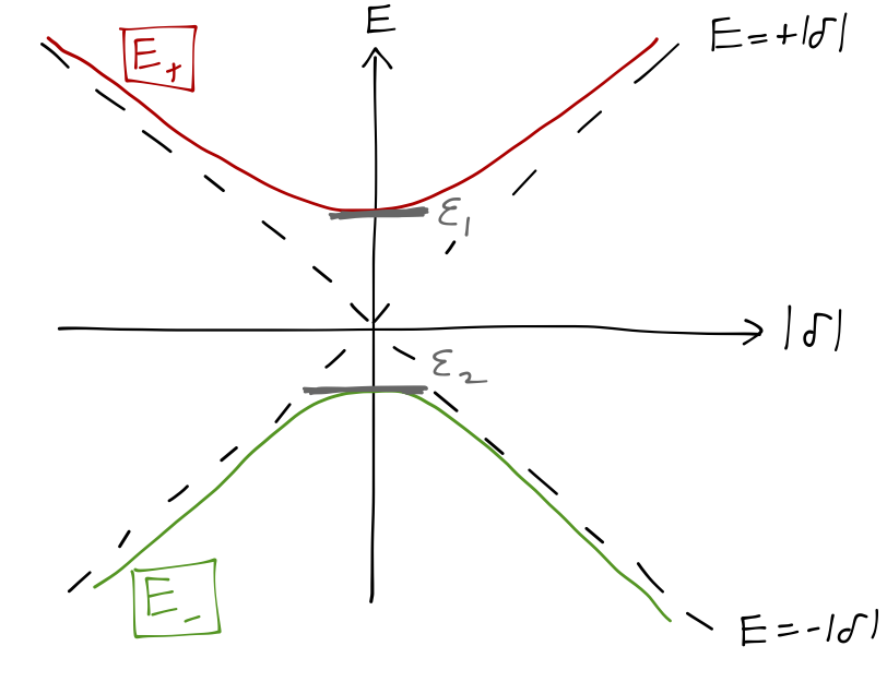
(This is a slightly funny plot since |\delta| is a norm and can’t be negative; you should interpret negative |\delta| on this plot as shifting the phase of \delta by \pi.)
This is an example of a phenomenon known as avoided level crossing. The two curves for \epsilon_1 and \epsilon_2 can never cross in this system, except in the special case where the splitting \epsilon = 0, where the eigenvalues become degenerate at \delta = 0. When the energies are degenerate, the system is in a state of enhanced symmetry; including either \epsilon or \delta breaks the symmetry, and there can be no level crossing. This is actually quite a general result, but this is just a preview; we can’t elaborate on the general no-crossing theorem until we study perturbation theory.
One other feature of note for the avoided level crossing: the sign of \delta is irrelevant for the energies, but it does affect the eigenstates. If the phase of \delta is shifted by \pi, then that’s the same as shifting the phase \phi in the eigenvectors by \pi. So the observation above about \ket{E_{\pm}} at |\delta| \gg \epsilon is true at positive |\delta| on the plot, whereas at negative |\delta| we have instead \ket{E_+} \rightarrow \frac{1}{\sqrt{2}} \left( \begin{array}{c} 1 \\ -1 \end{array} \right), \\ \ket{E_-} \rightarrow \frac{1}{\sqrt{2}} \left( \begin{array}{c} -1 \\ -1 \end{array} \right). \\ The overall sign is irrelevant, so we see that the states have swapped as we go from large, negative |\delta| to large, positive |\delta|. This is another generic feature of avoided level crossings.
4.3.1 Time evolution in the general case
So far, all I’ve done is solve for the energy eigenvalues and eigenvectors; we’ve seen some interesting things, but I haven’t said anything about computing time evolution. To come back to that, if we begin with an arbitrary initial state on the Bloch sphere: \ket{\psi(0)} = \cos (\theta_0/2) \ket{\uparrow} + \sin(\theta_0/2) e^{i\phi_0} \ket{\downarrow} what is \psi(t) given the most general Hamiltonian above? Since we have the eigenvectors and eigenvalues, the simplest approach is to expand in energy eigenvectors: we rewrite the state vector as
\ket{\psi(0)} = c_+ \ket{E_+} + c_- \ket{E_-}, and then simply write down the answer: \ket{\psi(t)} = c_+ e^{-iE_+ t/\hbar} \ket{E_+} + c_- e^{-iE_- t/\hbar} \ket{E_-}. What does this mean in practice? Well, what I’ve hidden in the c_\pm coefficients is that we had to do a change of basis as the first step from the initial \ket{\uparrow}/\ket{\downarrow} to the energy eigenvalues \ket{E_{\pm}}. The values of the coefficients are the inner products of the same quantum state \ket{\psi(0)} with different bases:
\left\langle \uparrow | \psi(0) \right\rangle = \cos (\theta_0/2), \left\langle - | \psi(0) \right\rangle = \sin(\theta_0/2) e^{i\phi_0}; \\ \left\langle E_+ | \psi(0) \right\rangle = c_+, \left\langle E_- | \psi(0) \right\rangle = c_-. To relate the coefficients, we just apply completeness: \left\langle E_+ | \psi(0) \right\rangle = \left\langle E_+ | \uparrow \right\rangle \left\langle \uparrow | \psi(0) \right\rangle + \left\langle E_+ | \downarrow \right\rangle \left\langle \downarrow | \psi(0) \right\rangle. We know all the numbers on the right-hand side: they are the Bloch sphere coordinates, and then the components of the energy eigenvector E_+ in the original \hat{S}_z basis.
I’m not going to write out the answer explicitly here - it will be messy in the most general case. Instead, I want to think about the procedure here, because this is an example of a common method for solving time evolution in quantum systems:
- Diagonalize the Hamiltonian;
- Change to the energy eigenbasis;
- Evaluate the time evolution (and if needed, change back.)
Diagonalization is exactly just solving for the eigenvectors and eigenvalues of \hat{H}; we know that this is powerful because time evolution in the energy eigenbasis is simple (energy eigenstates just pick up time-dependent phases.)
Although you can work all of this out just using bra-ket notation and completeness, it’s often simpler to see what is happening in matrix-vector notation, so let me briefly remind you about the details of changing bases now, and connect it to our bra-ket notation.
4.3.2 Change of basis
Let’s consider the general case where we have two different orthonormal basis sets \{ \ket{a}\} and \{ \ket{b} \} for a given Hilbert space. Since they are both bases, they have the same dimension N as our space and as each other.
For an arbitrary ket \ket{\psi}, we can begin by expanding it in the a basis as: \ket{\psi} = \sum_{i} \ket{a_i} \left\langle a_i | \psi \right\rangle. In vector notation, this can be written as \ket{\psi} = \left( \begin{array}{c} \left\langle a_1 | \psi \right\rangle \\ \left\langle a_2 | \psi \right\rangle \\ ... \\ \left\langle a_N | \psi \right\rangle \end{array} \right)_{a} where since we’re considering more than one basis now, I’m using a subscript to denote explicitly that this is a vector in the \{ \ket{a} \} basis. Similarly, in the \{ \ket{b} \} basis, we have \ket{\psi} = \left( \begin{array}{c} \left\langle b_1 | \psi \right\rangle \\ \left\langle b_2 | \psi \right\rangle \\ ... \\ \left\langle b_N | \psi \right\rangle \end{array} \right)_{b} How are the vector components related? We can just insert a complete set of states: \left\langle b_i | \psi \right\rangle = \sum_j \left\langle b_i | a_j \right\rangle \left\langle a_j | \psi \right\rangle \\ This formula is correct, but to connect on to matrix-vector notation, let’s write it in the form of a matrix-vector product in the a basis: \left\langle b_i | \psi \right\rangle \equiv \sum_j \bra{a_i} \hat{U}^\dagger \ket{a_j} \left\langle a_j | \psi \right\rangle. This is just rewriting so far, completely general, although my choice to call the operator \hat{U}^\dagger is anticipating what the answer will be. Comparing the two equations, we read off: \hat{U}^\dagger = \sum_k \ket{a_k} \bra{b_k}. Calling this the daggered operator is a choice of convention, but it ensures that the un-daggered operator directly relates the basis kets, i.e. \ket{b_i} = \hat{U} \ket{a_i}. It’s also straightforward to check that indeed \hat{U} is unitary (left as a quick exercise for you.) So going back to matrix notation, we see that we can translate our vectors from the original basis to the new basis by matrix multiplication with \hat{U}^\dagger: \left( \begin{array}{c} \left\langle b_1 | \psi \right\rangle \\ \left\langle b_2 | \psi \right\rangle \\ ... \\ \left\langle b_N | \psi \right\rangle \end{array} \right)_{b} = \left( U^\dagger \right) \left( \begin{array}{c} \left\langle a_1 | \psi \right\rangle \\ \left\langle a_2 | \psi \right\rangle \\ ... \\ \left\langle a_N | \psi \right\rangle \end{array} \right)_{a}. A similar derivation for the matrix elements of an operator \hat{X} allows us to show that the new matrix representing \hat{X} is given by a similarity transformation of the old matrix, \hat{X} \rightarrow \hat{U}{}^\dagger \hat{X} \hat{U}.
Prove that \hat{X} transforms to \hat{U}^\dagger \hat{X} \hat{U} under a change of basis, using completeness and the other definitions above.
Answer:
(to be filled in; check back later!)
Notice that for both matrices and vectors, \hat{U}{}^\dagger is always on the left. The reason that we multiply our state vectors by \hat{U}{}^\dagger and not by \hat{U} is that we’re thinking of this as a passive transformation; if the basis rotates according to \hat{U}, then the components of a state vector are rotated the opposite way. This is ultimately a choice of convention, so be wary of how things are defined in other references!
A unitary transformation preserves the norm of all of our kets; we can think of it as a rotation in the Hilbert space. In fact, operators have a property which is also invariant under unitary transformations, called the trace {\rm Tr} (\hat{X}), {\rm Tr} (\hat{X}) \equiv \sum_n \bra{a_n} \hat{X} \ket{a_n}. In other words, the trace of an operator is just the trace (sum of the diagonal components) of its matrix representation, in any orthonormal basis. From our definitions, the trace obviously maps to itself under a basis change: {\rm Tr} (\hat{X}) \rightarrow \sum_n \bra{a_n} \hat{U} (\hat{U}^\dagger \hat{X} \hat{U}) \hat{U}^\dagger \ket{a_n} = \sum_n \bra{a_n} \hat{X} \ket{a_n}.
The trace has some useful properties: {\rm Tr} (\hat{X} \hat{Y} \hat{Z}) = {\rm Tr} (\hat{Z} \hat{X} \hat{Y}) = {\rm Tr} (\hat{Y} \hat{Z} \hat{X})\ \ \textrm{(cyclic permutation)} \\ {\rm Tr} (\ket{a_i}\bra{a_j}) = \delta_{ij} \\ {\rm Tr} (\ket{b_i}\bra{a_i}) = \left\langle a_i | b_i \right\rangle.
4.3.3 Diagonalization
All of the above is useful, but requires us to specify our new basis \{ \ket{b_i} \} explicitly. More generally, we can use the standard procedure for finding matrix eigenvalues and eigenvectors in order to find a clever basis, constructing a \hat{U} which will diagonalize any given Hermitian operator.
Suppose that we’re working in a basis \{\ket{a}\}, in which operator \hat{B} is not diagonal. The eigenvectors of \hat{B} will satisfy the equation \hat{B} \ket{b} = b \ket{b} \\ \sum_i \hat{B} \ket{a_i} \left\langle a_i | b \right\rangle = b \sum_i \ket{a_i} \left\langle a_i | b \right\rangle \\ \sum_i \bra{a_j} \hat{B} \ket{a_i} \left\langle a_i | b \right\rangle = b \sum_i \left\langle a_j | a_i \right\rangle \left\langle a_i | b \right\rangle \\ \sum_i \left( \bra{a_j} \hat{B} \ket{a_i} - b \delta_{ij} \right) \left\langle a_i | b \right\rangle = 0. This is exactly the matrix eigenvalue equation; it has a solution only if \det(\hat{B} - b \hat{I}) = 0. For an N-dimensional Hilbert space, this is an N-th order polynomial equation with N (not necessarily distinct) solutions for b, which are the eigenvalues. Solving for the eigenvalues and then eigenvectors in the standard way, the change of basis matrix is \hat{U} = \left( \begin{array}{cccc} &&&\\ &&&\\&&&\\ &&&\\ \ket{b_1} & \ket{b_2} & ... & \ket{b_N} \\ &&&\\ &&&\\ &&&\\ &&& \end{array}\right)_a i.e. it is constructed by stacking the eigenvectors as columns. You should already know how to do all of this; I’m just reminding you of the details and telling you that the procedure with operators is completely standard.
One final word: although the eigenvectors of an operator obviously depend on our basis, the eigenvalues do not, i.e. the operators \hat{A} and \hat{U}{}^\dagger \hat{A} \hat{U} have the same eigenvalues. Two operators related by such a transformation are known as unitary equivalent; the proof that their spectrum (set of eigenvalues) is identical is in Sakurai. Many symmetries can be stated in terms of unitary operators, for example, we will see that spatial rotations can be expressed as a unitary operator, from which we could predict that the various spin-component operators in the Stern-Gerlach experiment had exactly the same eigenvalues \pm \hbar/2.
Just to be explicit, let’s finish up the two-state system with our new formalism. From our results above, the change of basis matrix from the \hat{S}_z basis to the energy eigenbasis is
\hat{U}_{z \rightarrow E} = \left( \begin{array}{cc} &\\ \ket{E_+} & \ket{E_-}\\ &\\ \end{array}\right) \\ = \left( \begin{array}{cc} \cos (\theta/2) & -\sin(\theta/2) \\ \sin (\theta/2) e^{i\phi} & \cos (\theta/2) e^{i \phi} \end{array} \right) with e^{i\phi} = \delta^\star / |\delta| and \tan \theta = -2|\delta| / (\epsilon_1 - \epsilon_2) as we found above. We can use this to take an arbitrary initial state, transform to the energy eigenbasis, apply the simple diagonal time evolution, and then transform back. Or, we can apply this to the diagonal time-evolution operator in the energy eigenbasis and similarity transform back to find \hat{U}(t) in our \hat{S}_z eigenbasis. (Again, I won’t write any such formulas out explicitly, and you shouldn’t either! Just construct this matrix for your specific problem and then apply the coordinate changes.)