31 Semi-classical electromagnetism
Some of the previous examples we’ve considered have been only partly quantum mechanical: we’ve used a quantum treatment of matter (e.g. atoms), but a classical treatment of electromagnetism as a background field. This is known as a semi-classical treatment.
This is, of course, eventually inconsistent; if we push the theory too far in certain directions, things will break down as classical physics gives way to quantum behavior. All of this is fixed by a fully quantum treatment of the electromagnetic field (and eventually by also incorporating special relativity, leading us to quantum electrodynamics and quantum field theory.) We know that a fully quantum-mechanical treatment requires acknowledging that the electromagnetic field itself is quantized, with the quanta of radiation known as photons.
But there are many useful results we can obtain just using the semi-classical approach. In fact, one key result was actually obtained by Einstein back in 1917, before quantum mechanics. There are other very useful results we’ll be able to obtain for quantum systems from study of semi-classical electromagnetic effects. Just keep in mind that what we’re about to set up is not completely internally consistent, which may make some features of the theory seem a little bit strange or arbitrary.
31.1 Prelude: Radiation and Einstein coefficients
Following Einstein, let’s consider the possible interactions of radiation with matter. We’ll focus on transitions involving two states, \ket{1} and \ket{2}, arbitrarily choosing E_2 > E_1, and we’ll consider the interactions as a function of the frequency \omega of the radiation. If we assume that a single photon is involved and we have a single transition from initial state to final state, then there are three different processes possible:
- Spontaneous emission: \ket{2} \rightarrow \ket{1} + \gamma.
The energy of the photon in this case (and all cases) will be E_\gamma = E_2 - E_1; the decay rate is defined to be \Gamma_S = A_{12}. Note that this only works for \ket{2} \rightarrow \ket{1}, since the photon has to have positive energy; in other words, there is no A_{21}. This is a process with no classical analogue!
- Absorption: \ket{1} + \gamma \rightarrow \ket{2}.
Here we do have a classical analogue, which is illuminating a system with a classical electromagnetic field. The transition rate should be proportional to the power of the radiation field; the photon is an input, and the more photons we send in per second, the faster the process will be. To parameterize this, we’ll work with the spectral energy density, u_\omega = du/d\omega, where u itself is the energy per unit volume. We use the spectral form instead of the straight energy density since we want to talk about rates at specific frequencies, rather than integrated over all photon frequencies. We write the absorption rate, then, as \Gamma_A = B_{21} u_\omega(\omega). (For a monochromatic electromagnetic wave, u_\omega is related to the time-averaged magnitude of the Poynting vector |\vec{S}|; more on that below.) Since the left-hand side \Gamma_A is a decay rate (1/time), and u_\omega has units of energy * time / volume, this means that B_{21} itself must have units of volume / energy / time{}^2.
- Stimulated emission: \ket{2} + \gamma \rightarrow \ket{1} + 2\gamma.
Once again, in this case we should find a rate proportional to the power, since there must be an incoming photon in order for this process to happen. However, the difference from absorption is that now the transition is down to the lower-energy state. The rate for this process is given by \Gamma_E = B_{12} u_\omega(\omega).
Since I find it confusing myself (partly due to an accumulation of somewhat odd definitions due to historical precedents, especially relating to astronomy), here I collect together some definitions related to the question: “how much light is there in our system?” (The relevant Wikipedia page may help, although it sets my personal record for how many times I’ve seen the word “confusing” or “confusion” appearing on one article…)
In statistical mechanics, a natural choice might be the energy density, with units of energy / volume. In the context of electromagnetism, this is typically denoted as u. For a thermal bath of photons, energy density is described by the Planck distribution, u_\omega(\omega, T) = \frac{8\pi h\nu^3}{c^3} \frac{1}{e^{h\nu / (k_B T)} - 1} = \frac{\hbar \omega^3}{\pi^2 c^3} \frac{1}{e^{\hbar \omega/(k_B T)} - 1} converting between the ordinary frequency \nu and angular frequency \omega which we prefer to use in quantum mechanics. Except, this is not the energy density, this is the spectral energy density, which is the energy per volume, per unit frequency. It is a differential quantity, meaning that we integrate it over frequency to get the ordinary energy density: u = \int d\omega\ u_\omega(\omega).
(In fact, I knew this to do the conversion above, since there is an extra factor of 2\pi that is hidden in converting from d/d\nu to d/d\omega.) However, this isn’t always the most convenient quantity to use. If you’re interested in the light radiated by a star, what the photons are doing inside the star is irrelevant; only the photons emitted from the surface of the star are of interest. Similarly, in a quantum experiment we often have the situation where light is propagating freely through space for a long time, before interacting with a small target in some way. In either case, we want to remove one dimension (the interior of the star, or the direction of propagation of the light) and instead talk about energy per unit area.
In the context of stars, the spectral energy density can be conveniently replaced with a quantity known as the spectral radiance B_\omega, which describes energy per area, per unit time. The are related by B_\omega = \frac{c}{4\pi} u_\omega = \frac{\hbar \omega^3}{4\pi^3 c^2} \frac{1}{e^{\hbar \omega/(k_B T)}-1} with the 4\pi coming from a solid-angle integration. This is once again a differential quantity; integrating it gives B = \int d\omega\ B_\omega which is just the radiance, units of energy / area. (Strictly speaking, the SI units are energy / area / steradian, to help disambiguate the point I’m about to make, although I never liked solid angles as “units”…)
In the present context, we’re not interested in stars; in the second context mentioned of illuminating a target with a beam of light, we more naturally want to normalize to the area of our target/beam, and the integration over the full solid angle doesn’t make sense. This gives a slight but important difference in our definitions, which basically amounts to discarding the 4\pi from solid-angle integration but otherwise keeping our units fixed. This defines the more relevant quantity for us and Einstein, which is the spectral irradiance I_\omega, given by I_\omega = 4 \pi B_\omega = \frac{\hbar \omega^3}{\pi^2 c^2} \frac{1}{e^{\hbar \omega/(k_B T)} - 1}. which is once again differentially related to the plain irradiance, I = \int d\omega\ I_\omega. This is in physics often simply called intensity, although “intensity” has been used for a few too many things in science, so “irradiance” is more specific if you want to be careful.
One can formulate the Einstein coefficient argument in terms of spectral irradiance, but we’ve worked in terms of spectral density; I think it’s most natural since the argument ends up in statistical mechanics. But I wanted to collect all this here since it can be confusing, and irradiance/intensity is much more natural for many problems in experimental physics as I’ve said.
The three as-yet unknown quantities A_{12}, B_{21}, B_{12} are known as Einstein coefficients. Now, continuing to follow Einstein, we suppose that we have a system consisting of a large population of atoms and photons (say inside of a reflective cavity), so that everything is in thermal equilibrium. The equilibrium populations of the two atomic states are N_1 and N_2. But if the system is at equilibrium, then we know that the rates for transitions from \ket{1} to \ket{2} and vice-versa must be balanced: N_1 \Gamma_A = N_2 (\Gamma_S + \Gamma_E) \\ N_1 B_{21} u_\omega(\omega) = N_2 (A_{12} + B_{12} u_\omega(\omega)). If we solve this for the radiation energy density, we find u_\omega(\omega) = \frac{A_{12}}{\tfrac{N_1}{N_2} B_{21} - B_{12}} Now, this is a system at some finite temperature T, which means that by Boltzmann statistics, we know that \frac{N_1}{N_2} = e^{-(E_1-E_2)/(k_B T)}. We don’t know what the energy levels are, but we do know what their splitting is: conservation of energy tells us that E_2 - E_1 = E_\gamma = \hbar \omega. Plugging back in, we find that u_\omega(\omega) = \frac{A_{12}}{e^{\hbar \omega/(k_B T)}B_{21} - B_{12} }. This should look familiar; it is precisely the Planck distribution, which is the predicted blackbody distribution for photons in equilibrium at temperature T. Well, to be precise, it has precisely the right functional form to be the Planck distribution, which is u_{\omega}^{\rm Planck}(\omega) = \frac{\hbar}{\pi^2 c^3} \frac{\omega^3}{e^{\hbar \omega/(k_B T)} - 1}. For everything to match, then, the Einstein coefficients must satisfy the following relations between them: B_{12} = B_{21} \equiv B, \\ A_{12} = \frac{\hbar \omega^3}{\pi^2 c^3} B.
As a final check, you can verify that the units of the prefactor in front of B come out to (energy) (time) / (volume); above we said that B itself has units of (volume) / (energy) / (time){}^2, so the product matches 1/(time) for the rate A_{12}.
This is as far as Einstein could get, prior to the invention of quantum mechanics. Matching on to the Planck distribution is certainly a nice achievement, but it’s a little unsatisfying to use thermal equilibrium as our tool to study this process - in particular, A_{12} is a rate for spontaneous emission, which certainly shouldn’t care about whether our system is in a thermal bath or not! Moreover, this argument can’t give us the actual values for the rates we’re interested in, just these relations between them. Still, this was a landmark result, and a key test of quantum-mechanical theory including electromagnetism is to be able to reproduce the Einstein relations. We’ll plan to do just that as we develop our own treatment of electromagnetism here.
I should comment that something may seem backwards at this point, since the Einstein argument starts with photons, whereas I told you that semi-classical electromagnetism uses background radiation fields instead of photons. But the Einstein argument doesn’t really treat single-photon interactions fully; it requires a statistical mechanical ensemble, averaged over many photons, in order to reach its conclusions. This averaging is what makes it a semi-classical treatment.
31.2 Electromagnetism in CGS units
Since we’ll now be relying more heavily on electromagnetism, although I’ve used some formulas already, let’s next write out some basics of electromagnetism in the CGS (a.k.a. “Gaussian”) units that are commonly used for quantum mechanics, including by Sakurai. Maxwell’s equations in CGS are as follows: \begin{aligned} \nabla \cdot \vec{E} &= 4\pi \rho(\vec{x}) \\ \nabla \cdot \vec{B} &= 0 \\ \nabla \times \vec{E} + \frac{\partial \vec{B}}{\partial t} &= 0 \\ \nabla \times \vec{B} - \frac{1}{c} \frac{\partial \vec{E}}{\partial t} &= \frac{4\pi}{c} \vec{J} \\ \end{aligned} and the Lorentz force law for the force on a charge q is \vec{F} = q\vec{E} + \frac{q}{c} \vec{v} \times \vec{B} picking up an extra factor of c relative to SI. It will be often be useful to write our fields in terms of the electromagnetic potentials \phi and \vec{A}, which are related to the fields as \begin{aligned} \vec{E} &= \nabla \phi - \frac{1}{c} \frac{\partial \vec{A}}{\partial t}, \\ \vec{B} &= \nabla \times \vec{A}. \end{aligned} We know that the potentials are only defined up to gauge transformations, so we can pick a convenient gauge; we will adopt Coulomb gauge, \nabla \cdot \vec{A} = 0. For our current discussions, the most important solution to these equations is that for radiation in free space, so with \rho = \vec{J} = 0. In free space with \rho = 0 and with the Coulomb gauge condition, the scalar potential satisfies the equation \nabla^2 \phi = 0, which implies simply that \phi = 0. (The combination of \nabla \cdot \vec{A} = 0 and \phi = 0 is sometimes known as “radiation gauge”, although it’s really just Coulomb gauge with some extra conditions.)
With these conditions, the Maxwell equations imply that the vector potential itself satisfies the wave equation, \nabla^2 \vec{A} = \frac{1}{c^2} \frac{\partial^2 \vec{A}}{\partial t^2}, which yields the solution \vec{A}(\vec{x}, t) = A_0 \vec{\epsilon} \cos (\vec{k} \cdot \vec{x} - \omega t) where A_0 gives the field strength, \omega = c|\vec{k}| and \vec{\epsilon} is a unit polarization vector (so |\epsilon|^2 = 1.) Applying the Coulomb gauge condition to this solution gives \vec{k} \cdot \vec{\epsilon} = 0, so that the polarization vector must be transverse to the wave vector \vec{k} and has only two independent degrees of freedom. Going forwards to the electric and magnetic fields, we have for radiation \begin{aligned} \vec{E} &= -\frac{\omega}{c} A_0 \vec{\epsilon} \sin (\vec{k} \cdot \vec{x} - \omega t), \\ \vec{B} &= -A_0 (\vec{k} \times \vec{\epsilon}) \sin (\vec{k} \cdot \vec{x} - \omega t). \end{aligned}
An important quantity that was already referred to in our previous derivation was the energy density u, which is given in terms of the electric and magnetic fields by u = \frac{1}{8\pi} (|\vec{E}|^2 + |\vec{B}|^2). Substituting in using the fields above, we have for free radiation u = \frac{|A_0|^2}{8\pi} \left( \frac{\omega^2}{c^2} |\vec{\epsilon}|^2 + |\vec{k} \times \vec{\epsilon}|^2 \right) \sin^2 (\vec{k} \cdot \vec{x} - \omega t) \\ = \frac{|A_0|^2}{8\pi} \left( \frac{\omega^2}{c^2} + |\vec{k}|^2 \right) \sin^2 (\vec{k} \cdot \vec{x} - \omega t) We can simplify this by identifying \omega = c|\vec{k}| and then by doing a time average, which reduces the \sin^2(...) \rightarrow 1/2, leaving us with \bar{u} = \frac{|A_0|^2 \omega^2}{8\pi c^2}.
Thus, if we are dealing with radiation with a known energy density u(\omega), we can invert this equation to find the field normalization |A_0|.
Finally, in quantum mechanics, we remind ourselves that the appropiate Hamiltonian to include electromagnetism for a charge q with mass m is \hat{H} = \frac{1}{2m} \left( \hat{\vec{p}} - \frac{q}{c} {\vec{A}} \right)^2 + V_0(\hat{x}). Note that we put hats on the momentum and position operators, but not on the gauge potential since we’re working semi-classically and treating it as a background field, so we don’t have to worry about gauge invariance or kinematical momentum operators.
There is a term missing from the Hamiltonian I’ve written above, one which is rather important and that we’ve seen before, as long as our charge has spin, which is the coupling of the spin magnetic moment to the magnetic field: \hat{V}_\mu = -\hat{\vec{\mu}} \cdot \hat{\vec{B}} = -\frac{q}{mc} \hat{\vec{S}} \cdot \vec{B}.
Why am I not writing this above? In general, we should include it, but we can also make a quick estimate of how large this is compared to the term that we are keeping, in the context of our radiation solution. The size of the largest term in the Hamiltonian above is E_1 \sim \frac{q}{mc} \vec{p} \cdot \vec{A} \sim \frac{q p A_0}{mc} while the magnetic term corresponds to an energy of order E_2 \sim \frac{q}{mc} \vec{S} \cdot \vec{B} \sim \frac{\hbar k q A_0}{mc} and if we take the ratio, \frac{E_2}{E_1} \sim \frac{\hbar k}{p}. So we end up with a ratio of momentum scales, but what momenta are they? \hbar k is the momentum associated with the EM wave itself, corresponding to a wavelength of \lambda = (2\pi/k). On the other hand, p is the momentum of the atomic electron itself; its characteristic wavelength will be roughly set by the Bohr radius, so p/\hbar \sim 2\pi/a_0. Thus, \frac{E_2}{E_1} \sim \frac{a_0}{\lambda}.
The Bohr radius a_0 is about 0.05 nm, whereas typical photon wavelengths from atomic transitions are of order hundreds or thousands of nm. So at least for an initial, first-order perturbative treatment, we are certainly justified in ignoring the magnetic moment interaction. This observation will also be useful for some other approximations that we’ll make below.
(This is, schematically, the difference between the de Broglie wavelength of an electron with 10 eV of energy and the wavelength of a photon with 10 eV of energy. Up to factors of c, the Bohr radius is set by an energy scale which is the geometric mean of 10 eV with the electron rest-mass energy scale of 511 keV.)
31.3 Electromagnetic transition amplitudes
Now that we’ve reminded ourselves of the basics, let’s move on to see explicitly how electromagnetic fields show up in time-dependent perturbation theory. We can separate out the electromagnetic parts to treat them as our perturbation, writing \hat{H}_0 = \frac{\hat{\vec{p}}^2}{2m} + V_0(\hat{x}) and then \hat{V} = -\frac{q}{mc} (\hat{\vec{p}} \cdot \vec{A} + \vec{A} \cdot \hat{\vec{p}}) + \frac{q^2}{2mc^2} |\vec{A}|^2 Under normal circumstances, [\vec{\hat{p}}, \vec{A}] \neq 0 because \vec{A} is a function of the position operator \hat{x}. But since we’re working in Coulomb gauge, \nabla \cdot \vec{A} = 0 means that they do commute, which lets us simplify the first term. We’ll also drop the second term; if we’re perturbing in the field strength |\vec{A}|, then it will be second-order and we’ll just focus mainly on first-order interactions. Thus, we have for our perturbation \hat{V} \approx -\frac{q}{mc} \vec{A} \cdot \hat{\vec{p}} = -\frac{qA_0}{mc} \cos (\vec{k} \cdot \hat{\vec{x}} - \omega t) (\vec{\epsilon} \cdot \hat{\vec{p}}).
Now let’s write down the resulting first-order transition amplitude. The general formula is U_{fi}^{(1)}(t) = -\frac{i}{\hbar} \int_0^t dt' e^{-iE_f (t-t')/\hbar} \bra{f} \hat{V}(t) \ket{i} e^{-iE_i t'/\hbar} \\ = \frac{i}{\hbar} e^{-iE_f t/\hbar} \frac{qA_0}{mc} \int_0^t dt' e^{i\omega_{fi} t'} \bra{f} \cos (\vec{k} \cdot \hat{\vec{x}} - \omega t) (\vec{\epsilon} \cdot \hat{\vec{p}}) \ket{i}. where once again we define \omega_{fi} \equiv (E_f - E_i) / \hbar. As we did before for a harmonic perturbation, it’s helpful to split the cosine into two complex exponentials, which allows us to isolate two separate transitions. Following our previous results for harmonic perturbations, the key difference now is that the perturbation matrix element is different for the two terms: we see that U_{fi}^{(1)}(t) = -\frac{e^{-iE_f t/\hbar}}{2\hbar} \left[ V_{fi}^{(+)} \frac{1 - e^{-i(\omega_{fi} - \omega)t}}{\omega_{fi} - \omega} + V_{fi}^{(-)} \frac{1 - e^{-i(\omega_{fi} + \omega)t}}{\omega_{fi} + \omega} \right] where we then have for the matrix elements in position space V_{fi}^{(+)} = \frac{-i\hbar qA_0}{2mc} \int d^3x\ e^{i\vec{k} \cdot \vec{x}} \psi_f^\star(\vec{x}) (\vec{\epsilon} \cdot \nabla) \psi_i(\vec{x}), \\ V_{fi}^{(-)} = \frac{-i\hbar qA_0}{2mc} \int d^3x\ e^{-i\vec{k} \cdot \vec{x}} \psi_f^\star(\vec{x}) (\vec{\epsilon} \cdot \nabla) \psi_i(\vec{x}), \\ For later use, let’s define the “matrix-element integral” M_{fi}(\omega) to be M_{fi}(\omega) = \int d^3x\ e^{+i(\vec{n} \cdot \vec{x}) \omega/c} \psi_f^\star(\vec{x}) (\vec{\epsilon} \cdot \nabla) \psi_i(\vec{x}) with \vec{n} = \vec{k} / |\vec{k}| defining the direction of propagation of our radiation. Then the full matrix elements are V_{fi}^{(+)} = -\frac{i\hbar qA_0}{2mc} M_{fi}(\omega), \\ V_{fi}^{(-)} = -\frac{i\hbar qA_0}{2mc} M_{fi}(-\omega).
As in the simpler harmonic-perturbation case we saw before, the first term in the transition amplitude corresponds to absorption, dominating when \omega_{fi} \approx \omega \Rightarrow E_f = E_i + \hbar \omega, and the second term corresponds to stimulated emission, dominating when \omega_{fi} \approx \omega \Rightarrow E_f = E_i - \hbar \omega.
31.3.1 Absorption rate
Let’s go on to compute the rates, starting with absorption. Plugging in from before, W_{fi}^{(+)} = \frac{2\pi}{\hbar} \int dE_f |V_{fi}^{(+)}|^2 \rho_f(E_f) \delta(E_f - E_i - \hbar \omega). We need to be cautious about the integration, since the matrix element itself can depend on the energy E_f. To evaluate this more cleverly, we recall that there is also some frequency dependence in the matrix element, coming from the normalization of our radiation solution: |V_{fi}^{(+)}|^2 = \frac{\hbar^2 q^2}{4m^2 c^2} |A_0|^2 M_{fi}(\omega) = \frac{2\pi \hbar^2 q^2}{m^2 \omega^2} \bar{u}(\omega) M_{fi}(\omega) \\ = \frac{2\pi \hbar^2 q^2}{m^2 \omega^2} \int d\omega\ \bar{u}_\omega(\omega) |M_{fi}(\omega)|^2 Now we can go back to our expression for the rate and collapse the delta function by doing the d\omega integral instead. Using \delta(E_f - E_i - \hbar \omega) = \delta(\hbar \omega_{fi} - \hbar \omega) = \delta(\omega_{fi} - \omega) / \hbar, we have W_{fi}^{(+)} = \frac{4\pi^2 q^2}{m^2 \omega^2} \int dE_f \int d\omega\ \bar{u}_\omega(\omega) \delta(\omega_{fi} - \omega) \rho_f(E_f) |M_{fi}(\omega)|^2 \\ = \frac{4\pi^2 q^2}{m^2 \omega^2} \int dE_f\ \bar{u}_\omega(\omega_{fi}) \rho_f(E_f) |M_{fi}(\omega_{fi})|^2. In this form, this expression for the rate should remind you of our discussion of Einstein coefficients above. In particular, suppose we are interested in the situation described by Einstein in which we have two atomic states \ket{1}, \ket{2} interacting with radiation (which also means that the charged particle we’re interacting with is an orbital electron, mass m_e and charge e.) This causes the density of states to become discrete, \rho_f(E) = \delta(E - E_1) + \delta(E - E_2). Identifying i = 1 and f = 2 for absorption, the discrete density of states causes the final integral to collapse and forces \omega_{21} = \omega, and we have an expression for the absorption rate: \Gamma_A = W_{21}^{(+)} \sim \bar{u}_\omega(\omega) \frac{4\pi^2 q^2}{m^2 \omega^2} |M_{21}(\omega)|^2 \equiv \bar{u}_\omega(\omega) B_{21}, recovering the assumed form of the absorption rate from above, and also giving us an explicit quantum-mechanical formula for the Einstein coefficient! (This isn’t quite right yet, hence the \sim; for one thing, this is a rate for a beam of radiation coming from a specific direction, and we need to average over directions and polarizations to really match properly onto the stat-mech system that Einstein had in mind. But we’ll come back to that once we know how to evaluate the matrix element integral M_{21}(\omega).)
31.3.2 Stimulated emission rate
For stimulated emission, the calculation is very similar to what we did for absorption above, but with some signs reversed. Following the same steps, we end up with the result for the emission rate W_{fi}^{(-)} = \frac{4\pi^2 q^2}{m^2 \omega^2} \int dE_f\ \bar{u}_\omega(\omega_{if}) \rho_f(E_f) |M_{fi}(-\omega_{if})| with the definition \omega_{if} = -\omega_{fi}, which has to be positive since the applied \omega = -\omega_{fi} > 0 under the integral. There is an extra minus sign in the integral M as well.
To make use of this observation, we can now specialize to the case of stimulated emission with two discrete energy levels \ket{1}, \ket{2}. This time, we have to switch which state is the final state: we have i = 2 and f = 1 now. The relevant transition rate is thus \Gamma_S = W_{12}^{(-)} = \bar{u}_\omega(\omega) \frac{4\pi^2 q^2}{m^2 \omega^2} |M_{12}(-\omega)|^2 \equiv \bar{u}_\omega(\omega) B_{12} with \omega = \omega_{21} exactly as above due to the initial/final state swap. Once again this matches the expectation from above, and gives us a formula for the Einstein coefficient. But now from the definition of the matrix-element integral M, it’s easy to show with an integration by parts that M_{12}(-\omega) = -M_{21}(\omega)^\star which means that, comparing the formulas, B_{12} = B_{21}. Thus, we’ve reproduced one of the two predictions from the stat-mech argument above, purely from quantum mechanics! In fact, this is a consequence of a symmetry we’ve seen before: if we write out the relation between M integrals in terms of the matrix elements themselves, the relation that is needed for the Einstein coefficients to be equal is \bra{1} \hat{V} \ket{2} = -\bra{2} \hat{V} \ket{1}^\star which can be shown using time reversal, assuming that [\hat{\Theta}, \hat{V}] = 0 - i.e., assuming that time reversal is a good symmetry of electromagnetism.
If you’re paying close attention, you may have noticed that although our original description of stimulated emission was given in terms of photons being both absorbed and emitted, in our calculation here we never included any photon in the density of states; \rho_f(E_f) is taken just to describe the atomic states. Why is this correct? (We’ll even see below that for spontaneous emission, we can’t ignore the presence of the final-state photon…)
The short answer is that this is one of those uncomfortable details that I warned we might run into as part of working semi-classically. When described in a fully quantum theory at the level of single photons, stimulated emission is a process where one photon comes in at frequency \hbar \omega, and two photons come out. Similarly for absorption, one photon goes in and zero photons are present in the final state. But in the current calculation, we have a background EM field present. Physically, this represents a huge number of photons, so we don’t notice any changes at the level of single photons; the field is the same before and after.
31.3.3 Spontaneous emission rate
Our first-order treatment of perturbation by radiation above had two terms, absorption and stimulated emission. But we should also be able to describe the third type of interaction from Einstein’s argument, which is spontaneous emission (which was well-known to occur experimentally even in 1916.) For spontaneous emission, an external EM field is no longer needed, so it should be described by a different perturbation Hamiltonian. But it’s also still an electromagnetic transition; semi-classically, we think of the perturbation as now being provided by the electromagnetic field of the emitted photon. This means the perturbation is almost identical: \hat{V}_\gamma = -\frac{qA_\gamma}{mc} \cos (\vec{k} \cdot \hat{\vec{x}} - \omega t) (\vec{\epsilon} \cdot \hat{\vec{p}}). The only thing that has changed here is the field strength |\vec{A}|. Why does that have to be different? For the two cases above, the energy density u was constant, which makes sense for an external “space-filling” EM field. But to study this process where a single photon is emitted spontaneously, the energy contained in the field should be constant, which means the density should not be.
To proceed, we imagine that we’re working in a box of volume L^3, and (as in previous examples) we expect that dependence on L will cancel out of our final answers. We already know how to write things in terms of the time-averaged energy density \bar{u}; for a single photon, we impose the condition E = \hbar \omega = \bar{u} L^3 which means that the single-photon normalization is |A_0|^2 = \frac{8\pi c^2}{\omega^2} \bar{u} = \frac{8\pi c^2}{\omega^2} \frac{\hbar \omega}{L^3} = \frac{8\pi \hbar c^2}{\omega L^3}.
The other thing that we need is the density of states, since now we will include the presence of the final-state photon in our state sum. We have to do this because, although the energy of the photon will be fixed by the energy-conserving delta function in the rate, the direction of the photon in spontaneous emission is totally arbitrary, so we have to sum over emission directions. (This is as opposed to stimulated emission, in which the direction of the wave vector \vec{k} is fixed.) In this case, it’s more convenient to take our finite box to have periodic boundaries, in which case the photon mode number is related to the wave vector as \vec{k} = \frac{2\pi}{L} \vec{n} (this has an extra factor of 2 compared to the fixed-boundary case.) To get the density of states, then, we first have \int d^3n = \left( \frac{L}{2\pi} \right)^2 \int d^3k = \left( \frac{L}{2\pi} \right)^3 \int d\Omega \int dk\ k^2 splitting the \vec{k} integral up in spherical coordinates, but not doing the solid-angle integral yet. To convert to energy, we previously used E_k = \hbar^2 k^2 / (2m), but that obviously won’t work for a massless photon - this is a non-relativistic dispersion relation. Instead we should use the relativistic relation, which for photons is simply E = \hbar c k leaving us with \int d^3n = \left(\frac{L}{2 \pi \hbar c} \right)^3 \int d\Omega_k \int dE\ E^2. where I’m writing the solid angle with a k subscript to remind us that it correspond to the direction of the \vec{n} vector, i.e. the direction in which the photon is emitted. Now, if we do the solid-angle integral at this point, it kicks out a factor of 4\pi, and we can read off the density of states as \rho(E) = \frac{L^3}{2\pi^2 \hbar^3 c^3} E^2. However, we don’t want to do that integral just yet. In general, the only case in which we can just do the integral is when our system is fully rotationally invariant - remember, we don’t only care about \int d^3n, we want to integrate our perturbative matrix element over d^3n. If that matrix element isn’t fully rotationally invariant, then we should be more careful.
This is enough for us to go back to perturbation theory. Keeping the angular dependence (which adds back a 1/4\pi to the density of states we plug in), the rate for spontaneous emission can be written in the form W_{\gamma,fi}^{(-)} = \frac{2\pi}{\hbar} \int d\Omega_k \int dE_\gamma \int dE_f \rho_f(E_f) |V_{\gamma,fi}^{(-)}|^2 \frac{L^3}{8\pi^3 \hbar^3 c^3} E_\gamma^2 \delta(E_f - E_i + E_\gamma) where the density of states for the atomic final state \ket{f} also appears, along with the density for the photon. The perturbative matrix element here is |V_{\gamma,fi}^{(-)}|^2 = \frac{\hbar^2 q^2}{4m^2 c^2} \frac{8\pi \hbar c^2}{\omega L^3} |M_{fi}(-\omega)|^2 = \frac{2\pi \hbar^3 q^2}{m^2 \omega L^3} |M_{fi}(-\omega)|^2. where \omega \equiv E_\gamma / \hbar. As expected the dependence on the fictitious box size L cancels right away, and we have W_{\gamma,fi}^{(-)} = \frac{\hbar^2 q^2}{2\pi c^3 m^2 \omega} \int d\Omega_k \int d\omega\ \omega^2 \int dE_f \rho_f(E_f) M_{fi}(-\omega) \delta(E_f - E_i + \hbar \omega). trading out E_\gamma, taking us back to something that looks like what we had in the previous two cases. We can do the \omega integral as before: W_{\gamma,fi}^{(-)} = \frac{\hbar q^2}{2\pi c^3 m^2 \omega} \int d\Omega_k \int dE_f \rho_f(E_f) |M_{fi}(-\omega_{if})|^2 \omega_{if}^2. with \omega_{if} \equiv (E_i - E_f) /\hbar as above. Now, it’s important to note that although there is an angular integral being done inside the matrix element M_{fi}(\omega), there can still be residual angular dependence so that the d\Omega_k integral isn’t always trivial. (We will see this explicitly in an example; conceptually, the integral inside M_{fi} is over space given a fixed photon direction \vec{n} = \vec{k}/|\vec{k}|, while the external d\Omega_k integral is over the photon direction.) In fact, in general it’s more convenient to rewrite this as a differential rate, in the form \frac{dW_{\gamma,fi}^{(-)}}{d\Omega_k} = \frac{\hbar q^2}{2\pi c^3 m^2 \omega} \int dE_f \rho_f(E_f) |M_{fi}(-\omega_{if})|^2 \omega_{if}^2
Finally, we specify the density of states to be the two-state system we had before, setting E_f = E_1 and E_i = E_2, and find the result \frac{dW_{\gamma,21}}{d\Omega_k} = \frac{\hbar q^2 \omega}{2\pi c^3 m^2} |M_{21}(-\omega)|^2 and thus the final Einstein coefficient is (up to some averaging details we still need to fill in) A_{21} \sim \int d\Omega_k \frac{\hbar q^2 \omega}{2\pi c^3 m^2} |M_{21}(-\omega)|^2.
This matches the form we expect (in that it is independent of \bar{u}_\omega(\omega), basically by construction!), and it shares some factors with our results for B. In fact, if we take the ratio, we find that at least for the dimensionful quantities, \frac{A_{21}}{B_{21}} \sim \frac{\hbar \omega^3}{c^3} matching precisely the form expected in Einstein’s stat-mech argument. However, we don’t have the numerical factors quite right yet; to do that, we need to simplify further.
31.4 Dipole approximation
Now let’s continue to try to fill in what the matrix-element integral M_{21}(\omega) is. Knowing this will let us use these formulas beyond just the specific motivating stat-mech example, to really describe the details of individual atomic transitions.
Earlier in this chapter, we justified dropping the electron spin contribution to the electromagnetic Hamiltonian by arguing that it will be negligible, based on a large separation of energy scales. This argument boiled down to identifying a separation of length scales, that the wavelength \lambda of typical radiation involved in atomic transitions is much larger than the atoms themselves:
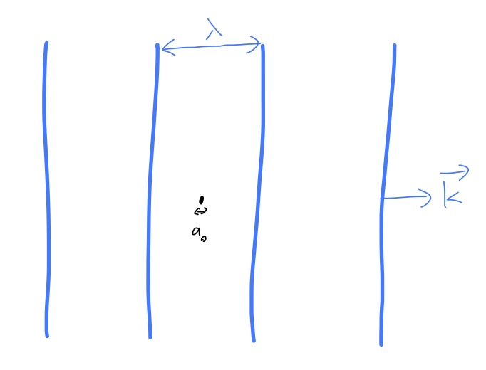
This means that over the distances scales of an atomic interaction, we can treat the electric and magnetic fields as if they are spatially constant. This means that we can evaluate the integral M_{fi}(\omega) by replacing the position-dependent phase e^{i\vec{k} \cdot \vec{x}} \rightarrow 1: M_{fi}(\omega) \approx \int d^3x \psi_f^\star(\vec{x}) (\vec{\epsilon} \cdot \nabla) \psi_i(\vec{x}). Notice that this replacement removes all of the \omega dependence from the integral. The remaining integral can be simplified with a nice trick that requires us first to lift back out of position space: M_{fi} = \vec{\epsilon} \cdot (\bra{f} \frac{i}{\hbar} \hat{\vec{p}} \ket{i}). Now, we can exploit the fact that \ket{i} and \ket{f} are energy eigenstates, together with remembering the fact that for any Hamiltonian of the form \hat{p}^2 / (2m) + V(\hat{x}), the Heisenberg equation of motion for \hat{\vec{x}} is especially simple: \hat{\vec{p}} = \frac{-i}{\hbar} m [\hat{\vec{x}}, \hat{H}] This lets us rewrite: \bra{f} \frac{i}{\hbar} \hat{\vec{p}} \ket{i} = \frac{m}{\hbar^2} \bra{f} [\hat{\vec{x}}, \hat{H}] \ket{i} = -\frac{m \omega_{fi}}{\hbar} \bra{f} \hat{\vec{x}} \ket{i}.
Thus, we have the result:
For radiation interacting with matter in the case where the radiation wavelength \lambda is very large compared to the size of the object, the matrix element for a transition \ket{i} \rightarrow \ket{f} is given by the dipole transition matrix element, M_{fi} = \frac{i}{\hbar} \bra{f} \vec{\epsilon} \cdot \hat{\vec{p}} \ket{i} = -\frac{m \omega_{fi}}{\hbar} \bra{f} \vec{\epsilon} \cdot \hat{\vec{x}} \ket{i} = -\frac{m \omega_{fi}}{\hbar} \vec{\epsilon} \cdot \int d^3x \psi_f^\star(\vec{x}) \vec{x} \psi_i(\vec{x}).
Since we have a couple of frequencies running around and it can be confusing, I’ll emphasize that this has become independent of the radiation frequency \omega; the frequency \omega_{fi} showed up through the Hamiltonian acting on the energy levels \ket{i}, \ket{f}.
This is called “dipole approximation” since the matrix element \bra{f} \hat{\vec{x}} \ket{i} is the same one that would show up for a charged dipole interacting with a background electric field. As we have discussed, it is a natural approximation to use for atomic transitions due to the separation of scales \lambda \gg a_0. It also happens to be exactly the approximation we would want to make in order to make sure our semiclassical treatment of light is valid! Long wavelengths mean (as we’ve seen) that the EM field is approximately static in our interactions, and the fact that the field is really quantized into photons is only really relevant when we consider its dynamics.
Another way to think of dipole approximation is that it comes from series expansion of the object e{i\vec{k} \cdot \vec{x}} appearing inside of M_{fi}: \bra{f} e^{\pm i\vec{k} \cdot \vec{x}} (\vec{\epsilon} \cdot \hat{\vec{p}}) \ket{i} \approx \bra{f} \left(1 \pm i\vec{k} \cdot \hat{\vec{x}} - \frac{1}{2} |\vec{k} \cdot \hat{\vec{x}}|^2 + ...\right) (\vec{\epsilon} \cdot \hat{\vec{p}}) \ket{i}
As we’ve already seen before, in some cases (depending on the specific states \ket{i}, \ket{f}) the dipole matrix element \bra{f} \vec{x} \ket{i} vanishes due to symmetry. In such cases, as long as we still have \vec{k} \cdot \vec{x} \ll 1, the dominant contribution will come from keeping the first non-vanishing term in the expansion.
31.4.1 Evaluating the Einstein coefficients
With this approximation in hand, we can simplify our results for the Einstein coefficients further. We’ll now deal with all the details properly. Let’s begin with absorption. For a given frequency \omega = \omega_{21}, we found the result B_{21} \sim \frac{4\pi^2 q^2}{m^2 \omega^2} |M_{21}(\omega)|^2. The \sim reminds us that this isn’t quite the complete answer; the reason is that it was calculated for a fixed light direction \vec{n} and polarization \vec{\epsilon}, whereas in the context of a stat-mech system of atoms and radiation, we should average over all directions and all polarizations: B_{21} = \frac{4\pi^2 q^2}{m^2 \omega^2} \frac{1}{4\pi} \int d\Omega_k \frac{1}{2} \sum_{\epsilon} |M_{21}(\omega)|^2 \\ = \frac{\pi q^2}{2m^2 \omega^2} \int d\Omega_k \sum_{\epsilon} \left| \frac{-m \omega}{\hbar} \bra{f} \vec{\epsilon} \cdot \vec{x} \ket{i} \right|^2, applying the dipole approximation.
In this example, we average over the two orientations of the polarization vector, which means we pick up an extra factor of 1/2 in front of the sum. The average is done to deal with our uncertainty over the direction of the polarization vector for photons in the isotropic gas we are considering. But in other cases, in particular for spontaneous emission which we’ll consider below, an unknown polarization state is dealt with by summing over polarizations - not including the factor of 1/2.
We can understand the difference in terms of density matrices. Classically, the polarization of our radiation is represented by a normalized two-component vector, \vec{\epsilon} = a \vec{\epsilon}_1 + b \vec{\epsilon}_2. In a quantum mechanics, this means that the polarization is described by a two-state Hilbert space spanned by \ket{\epsilon_1} and \ket{\epsilon_2}. Unpolarized light in quantum mechanics, then, is light with a density matrix which represents maximum uncertainty about the polarization vector: \hat{\rho}_{\rm unpol} = \frac{1}{2} \ket{\epsilon_1}\bra{\epsilon_1} + \frac{1}{2} \ket{\epsilon_2}\bra{\epsilon_2} If we have an observable that depends on polarization, we thus see that its expectation value is given by {\rm Tr} (\hat{\rho}_{\rm unpol} \hat{O}(\epsilon)) = \frac{1}{2} \sum_{\epsilon} \left\langle \hat{O}(\epsilon) \right\rangle.
In other words, as we’ve learned from density matrices, classical uncertainty about polarization in the initial state results in an average over the polarization vector in our observable.
On the other hand, if we don’t know the final-state polarization of our radiation, that simply means that we’re not measuring it, which means that whatever measurement we are doing acts as the identity matrix on the polarization subspace: \hat{O}_{\rm unpol} = \hat{O} \otimes \hat{1}_{\epsilon} = \hat{O} \otimes (\ket{\epsilon_1}\bra{\epsilon_1} + \ket{\epsilon_2}\bra{\epsilon_2}) which is a sum, not an average - so no extra factor to normalize.
The rule of thumb to remember is, generally: average over initial states, sum over final states.
Now we need to evaluate the polarization sum, for which we can derive a simple identity: \sum_{\epsilon} |\vec{\epsilon} \cdot \vec{v}|^2 = |\vec{\epsilon}_1 \cdot \vec{v}|^2 + |\vec{\epsilon}_2 \cdot \vec{v}|^2 \\ = |v_1|^2 + |v_2|^2 \\ = |v_1|^2 + |v_2|^2 + |v_3|^2 - |v_3|^2 \\ = |\vec{v}|^2 - \frac{|\vec{v} \cdot \vec{k}|^2}{|\vec{k}|^2} \\ = |\vec{v}|^2 (1 - \cos^2 \theta_k), where \theta_k is the opening angle between \vec{v} and \vec{k}. Plugging back in above, then, we have
B_{21} = \frac{\pi q^2}{2\hbar^2} \int d\Omega_k (1 - \cos^2 \theta_k) |\bra{f} \hat{\vec{x}} \ket{i}|^2 \\ = \frac{4\pi^2 q^2}{3\hbar^2} |\bra{f} \hat{\vec{x}} \ket{i}|^2.
Now we need to simplify the other coefficient for spontaneous emission: A_{21} = \frac{\hbar \omega q^2}{2\pi m^2 c^3} \int d\Omega_k \sum_{\epsilon} |M_{21}(\omega)|^2 \\ = \frac{\hbar \omega q^2}{2\pi m^2 c^3} \int d\Omega_k \sum_{\epsilon} \left| -\frac{m \omega}{\hbar} \bra{f} \vec{\epsilon} \cdot \hat{\vec{x}} \ket{i} \right|^2 \\ = \frac{\omega^3 q^2}{2\pi \hbar c^3} \int d\Omega_k (1 - \cos^2 \theta_k) |\bra{f} \hat{\vec{x}} \ket{i}|^2 \\ = \frac{4\omega^3 q^2}{3\hbar c^3} |\bra{f} \hat{\vec{x}} \ket{i}|^2 doing the sum and integration exactly as above. Note that in this case, because the photon is only in the final state, we sum instead of averaging over polarization and over direction.
Taking the ratio of these final results, we recover precisely the relation from Einstein’s argument precisely: \frac{A_{21}}{B_{21}} = \frac{\hbar \omega^3}{\pi^2 c^3}, But better yet, we can now compute the coefficients A_{21} and B_{21} from first principles for a given atomic transition!
31.5 Example: absorption of EM radiation by an atom
Let’s try one other example application, aside from the Einstein coefficients, before we move on. Our result for absorption in a generic atomic transition took the form: W_{i \rightarrow n} = \frac{2\pi}{\hbar^2} \int dE_n |V_{ni}^{(+)}|^2 \rho_f(E_n) \delta(\omega_{ni} - \omega) Going back a step, the transition matrix element in dipole approximation is V_{ni}^{(+)} \approx \frac{eA_0}{2mc} im\omega_{ni} \bra{n} \vec{\epsilon} \cdot \hat{\vec{x}} \ket{i} so |V_{ni}^{(+)}|^2 = \frac{e^2 \omega_{ni}^2}{4\hbar^2 c^2} |A_0|^2 |\bra{n} \vec{\epsilon} \cdot \hat{\vec{x}} \ket{i}|^2, or going back to the rate, W_{i \rightarrow n} = \frac{\pi e^2}{2\hbar^2 c^2} \int dE_n |A_0|^2 \omega_{ni}^2 |\bra{n} \vec{\epsilon} \cdot \hat{\vec{x}} \ket{i}|^2 \rho_f(E_n) \delta(\omega_{ni} - \omega).
For this process, rather than working with just the transition rate itself, let’s define an absorption cross-section, \sigma_{\rm abs} \equiv \frac{E_{\rm src} W_{i \rightarrow n}}{|\vec{S}_{\rm src}|}. Notice that the cross section has units of (energy/time) divided by (energy/area * time) = area. Two things to point out: first, this is a more natural quantity to work with for a particle scattering experiment - working with the Poynting vector makes sense if we are running an experiment with a beam applied in a fixed direction with fixed intensity and energy. Second, the cross-section is defined in such a way that the details of our experiment, E_{\rm src} and \vec{S}_{\rm src}, are divided out. This allows us to capture something which we can really think of as an intrinsic property of the target system, independent of how intense our laser beam is.
Returning to our specific example, the Poynting vector in CGS units takes the general form |\vec{S}| = \frac{c}{4\pi} |\vec{E} \times \vec{B}| We’d like to work in terms of the time average for our oscillating radiation solution again. Expanding this out using some vector-calc identities for our radiation solution and then taking a time average as before yields the result \left\langle |\vec{S}| \right\rangle = \frac{c}{8\pi} |E_0|^2 = \frac{|A_0|^2 \omega^2}{8 \pi c}.
Making the replacement of a discrete set of energy levels \rho(E_i) \rightarrow \sum_n \delta(E_n - E_i - \hbar \omega), the rate becomes W_{i \rightarrow n} = \frac{\pi e^2}{2\hbar^2 c^2} \frac{8\pi c \left\langle |\vec{S}| \right\rangle}{\omega^2} |\bra{n} \vec{\epsilon} \cdot \hat{\vec{x}} \ket{i}|^2 \sum_n \omega_{ni}^2 \delta(\omega_{ni} - \omega) so that the absorption cross-section becomes \sigma_{\rm abs}(\omega) = \frac{(\hbar \omega) W_{i \rightarrow n}}{\left\langle |\vec{S}| \right\rangle} \\ = 4 \pi^2 \frac{e^2}{\hbar c} \omega |\bra{n} \vec{\epsilon} \cdot \hat{\vec{x}} \ket{i}|^2 \sum_n \delta(\omega_{ni} - \omega) \\ = 4\pi^2 \alpha \omega |\bra{n} \vec{\epsilon} \cdot \hat{\vec{x}} \ket{i}|^2 \sum_n \delta(\omega_{ni} - \omega).
Since the source is at a fixed frequency \omega, the sum doesn’t really matter (up to possible counting factors from degenerate states), since \omega has to be tuned to pick up a specific energy level E_n and the contribution from all other final states \ket{n} is zero.
While this is a complete description (in dipole approximation) given a plane wave with fixed frequency \omega, in a more realistic situation we would probably be illuminating our atom with a light source that has some frequency distribution, meaning we don’t need to tune exactly to the transition frequency \omega_{ni}.
We can also ask about what happens if we sum over all possible source frequencies. This defines the total cross-section for absorption, \sigma_{\rm abs, tot} = \int d\omega \sigma_{\rm abs}(\omega) \\ = \sum_n 4\pi^2 \omega_{ni} |\bra{n} \hat{z} \ket{i}|^2. Now, we define a quantity known as the “oscillator strength”, f_{ni} \equiv \frac{2m_e}{\hbar} \omega_{ni} |\bra{n} \hat{z} \ket{i}|^2. It turns out that, by the Thomas-Reiche-Kuhn sum rule (which you proved on the homework, and which follows from the observation that [\hat{z}, [\hat{z}, \hat{H}_0]] = 0), these satisfy the identity \sum_n f_{ni} = 1. This means that we can simplify the sum above: pulling out some constant factors, we see that \sigma_{\rm abs, tot} = \frac{4\pi^2 \alpha \hbar}{2m_e} = \frac{2\pi^2 e^2}{m_e}. As is evident from the factor of \hbar cancelling out, this is a classical electrodynamics result! (But as such, it’s also a good check that we’ve set up all our formalism correctly.)