19 WKB approximation
Exactly solvable systems are something of a rare and special case in quantum mechanics (and in most of physics, really.) Now that we’ve seen all of the basic ideas, we’re ready to start our study of approximation methods that will let us study a much wider range of physical systems and phenomena, at the cost of having to settle for approximate solutions and expansions in small parameters. This is a very minor cost in exchange for what we get: actually being able to write down solutions to real physics problems!
Before we get to other, more general methods, let’s start in one-dimensional wave mechanics with the WKB approximation (named after its inventors: Wentzel, Kramers, and Brillouin.) There are various approximation methods useful for solving differential equations in general, but WKB is particular to quantum mechanics, based on a semi-classical expansion (with “semi-classical” roughly meaning expansion in \hbar, but we’ll see below that the precise details are a little more nuanced.)
19.1 Solving in WKB approximation
Let’s start by writing down Schrödinger’s equation in one dimension with an arbitrary potential: \frac{d^2 \psi_E}{dx^2} + \frac{2m}{\hbar^2} (E-V(x)) \psi_E(x) = 0. If V(x) is constant, then we’ve already seen that we can easily find solutions as complex exponentials, with the wave number determined by the difference E-V. The key idea behind WKB approximation is that for a potential that is almost constant (with “almost constant” to be defined more precisely below), the solutions will still be complex exponentials, but with a wave number k(x) that depends on position. We define k(x) = \left[ \frac{2m}{\hbar^2} (E-V(x)) \right]^{1/2}, and then the Schrödinger equation can be rewritten simply as \frac{d^2 \psi_E}{dx^2} + [k(x)]^2 \psi_E(x) = 0. Now let’s try the ansatz that \psi_E(x) = \exp \left[ i W(x) / \hbar \right] and see what happens (we know this has to work in the limit that k(x) becomes constant.) Plugging back in gives us an equation for W(x), i \hbar \frac{d^2 W}{dx^2} - \left( \frac{dW}{dx} \right)^2 + [p(x)]^2 = 0, where p(x) = \hbar k(x). Unfortunately, we can’t actually solve this equation in general. However, we know that it is solvable in certain cases at least: namely, with a constant potential we have W(x) = \hbar kx, which trivially gives us back p(x) = \hbar k since the second derivative vanishes.
This gives us a big hint as to how we should proceed: we can see that if the second-derivative term vanishes in general, we can solve for W(x) simply by integrating the wave number k(x). Instead of requiring it to exactly vanish, we can just consider the case where it is negligible compared to the first derivative term, \hbar \left| \frac{d^2 W}{dx^2} \right| \ll \left| \frac{dW}{dx} \right|^2. The obvious way to guarantee this condition is to work in the semi-classical limit, i.e. by expanding in small \hbar. Since \hbar is dimensionful, this immediately raises the question “small compared to what?” - but let’s just expand in \hbar first, and then we’ll study the validity of our solutions and find a more physical condition. Writing our solution for W(x) as a power series in \hbar, we have W(x) = W_0(x) + \hbar W_1(x) + \hbar^2 W_2(x) + ...
Beware: if you have read the derivation of the WKB approximation in Sakurai, he has secretly done this and then recombined terms, so his W_1(x) is equal to my W_0(x) + \hbar W_1(x). Shankar and other textbooks give a more standard derivation. Of course, what you should beware of in our current approach is that W_0, W_1, W_2... all have different dimensions!
Plugging back in to the Schrödinger equation and keeping only the first few terms in the expansion, we find \left[ - W_0'(x)^2 + p(x)^2 \right] \hbar^0 + \left[ i W_0''(x) - 2 W_0'(x) W_1'(x) \right] \hbar + \mathcal{O}(\hbar^2) = 0. At leading order in \hbar, dropping the second term completely, we find that we just have to integrate to find our approximate solution, W_0'(x) = \pm p(x) and then W_0(x) is simply given by the integral W_0(x) = \int dx\ \hbar k(x). We can do better than this, however; the next term is still not too bad to work with. Each term order by order in the \hbar expansion must vanish independently, so we still have W_0'(x) = p(x), and therefore W_0''(x) = \pm p'(x). Solving the second expression for W_1'(x) then yields -2i W_1'(x) = \frac{W_0''(x)}{W_0'(x)} = \frac{p'(x)}{p(x)} or integrating both sides, -2i W_1(x) = \log p(x) + C \\ \Rightarrow W_1(x) = i \log \sqrt{p(x)} + C'. Putting our two solutions back together and integrating over W_0'(x), we have \psi_E(x) \approx \exp \left[ \frac{i}{\hbar} (W_0(x) + \hbar W_1(x) ) \right] \\ = \frac{1}{\sqrt{p(x)}} \exp \left[ \pm \frac{i}{\hbar} \int^x dx'\ p(x') \right] \\ = \frac{1}{\sqrt{2m(E-V(x))}} \exp \left[ \pm \frac{i}{\hbar} \int^x dx' \sqrt{2m(E-V(x'))} \right], writing the wave number k(x) out explicitly. In general, we usually work compactly with either k(x) or the counterpart which is real when the energy is less than the potential: i.e., we define k(x) = \left[ \frac{2m}{\hbar^2} (E-V(x)) \right]^{1/2}, \\ \kappa(x) = \left[ \frac{2m}{\hbar^2} (V(x)-E) \right]^{1/2}, and then the form of the general solution under WKB looks just like our plane-wave or real-exponential solutions, just with additional position dependence.
Solutions to the Schrödinger equation under the WKB approximation can be written in the form \psi_E(x) \approx \begin{cases} \frac{1}{\sqrt{k(x)}} \exp \left[ \pm i \int^x dx' k(x') \right],& E > V(x); \\ \frac{1}{\sqrt{\kappa(x)}} \exp \left[ \pm \int^x dx' \kappa(x') \right],& E < V(x), \end{cases} with the position-dependent wave numbers k(x) and \kappa(x) defined as above. The funny-looking limit on this integral is a reminder that we don’t care about the overall normalization of this solution, since it’s multiplied by an arbitrary constant; we can pick any lower limit we want as long as we’re consistent.
As usual, there are two solutions, and the most general solution to the differential equation is a linear combination with arbitrary coefficients, e.g.~\psi_E(x) \sim A/\sqrt{k(x)} e^{i \int^x dx' k(x')} + B/\sqrt{k(x)} e^{-i \int^x dx' k(x')}.
What we’ve done here is a truncation: we’re ignoring all of the higher-order terms W_2(x), W_3(x), ... on the assumption that they are “small” (linked to the idea that in some sense \hbar is “small”.) If we’ve made a good assumption, then our series should be converging rapidly to the correct solution, i.e. we should find that \hbar W_1(x) \ll W_0(x). Let’s check: i \hbar \log \sqrt{p(x)} \ll \int^x dx' p(x'), \\ i \hbar \int^x dx' \frac{p'(x')}{p(x')} \ll \int^x dx' p(x'), Since we’re doing the same integral on both sides, the inequality will thus be satisfied as long as |k'(x)| \ll |k(x)^2| (where the absolute value lets us deal with the E < V(x) case in a compact way.) We can interpret this condition physically by defining a position-dependent de Broglie wavelength, \lambda(x) \equiv \frac{2\pi}{k(x)}. Since \lambda'(x) = -\frac{2\pi k'(x)}{k(x)^2}, we can see that our consistency condition for the WKB approximation is just that \left| \frac{d\lambda}{dx} \right| \ll 1 (ignoring the constant factors.) This can be usefully rewritten by noting that \lambda'(x) = -\lambda(x) \frac{p'(x)}{p(x)} \\ p'(x) = \frac{V'(x)}{2\sqrt{2m(E-V(x))}} = \frac{V'(x)}{p(x)} and so the condition becomes \lambda(x) \left| \frac{dV}{dx} \right| \ll \frac{[p(x)]^2}{m}. Thus, WKB is valid when the potential energy is changing slowly (in units of the local wavelength), compared to the kinetic energy. This is generally referred to as “slow variation” of the potential energy, now defined precisely.
This is a good quantitative condition, but what does this have to do with the semiclassical limit? If we work with the momentum p(x) and take \hbar \rightarrow 0, then the de Broglie wavelength \lambda = 2\pi \hbar / p also goes to zero, in which case all potential energy functions become slowly varying. The yardstick that determines what “slowly varying” means in any given problem is just the de Broglie wavelength.
Let’s consider the example of a sinusoidal potential of the form V(x) = V_0 \sin(k_0 x). Let’s look for solutions with E > V_0, so they are strictly oscillating; we then need to further insist that \lambda_0 = 2\pi / k_0 is very large compared to \lambda(x) , which means that k_0 \ll k(x) = \frac{\sqrt{2m}}{\hbar} \sqrt{E-V_0 \sin(k_0 x)}. In particular, for a fixed k_0 taking E very large will do the trick by making the wavefunction oscillate rapidly. With these restrictions, we’re free to solve in the WKB approximation. We need to do an integral first: \int^x dx\ k(x) = \sqrt{\frac{2mE}{\hbar^2}} \int_0^x dx\ \sqrt{1 - \frac{V_0}{E} \sin(k_0 x)}. The bad news is that this is an elliptic integral in general, so we can’t do it exactly. But if we’re working in the limit E \gg V_0, then we can series expand in the ratio \xi \equiv V_0 / E: \int^x dx\ k(x) \approx \sqrt{\frac{2mE}{\hbar^2}} \int_0^x dx\ \left( 1 - \frac{\xi}{2} \sin(k_0 x) \right) \\ = k_E x + \frac{\xi k_E}{2k_0} \cos(k_0 x) + \mathcal{O}(\xi^2), where k_E \equiv \sqrt{2mE/\hbar^2} is the wave number neglecting V_0. Some caution is required here because the ratio k_E / k_0 is by assumption large and not small; however, since \xi \sim 1/E while k_E \sim \sqrt{E}, we see that the second term will still vanish as E \rightarrow \infty, so our expansion is okay.
Now we can write down the general solution: \psi_{WKB}(x) = \frac{A}{\sqrt{k(x)}} \exp \left( ik_E x + i\xi \frac{k_E}{2k_0} \cos(k_0 x) \right) + \frac{B}{\sqrt{k(x)}} \exp \left( -ik_E x -i\xi \frac{k_E}{2k_0} \cos(k_0 x) \right) \\ \approx \frac{A}{\sqrt{2m(E-V_0 \sin(k_0 x))}} e^{ik_E x} \left(1 + i \xi \frac{k_E}{2k_0} \cos(k_0 x) \right) + ... where k_E \equiv \sqrt{2mE/\hbar^2} is the wave number neglecting V_0. Clearly if we take \xi \rightarrow 0, removing the potential completely, we just recover the simple plane-wave solution; the first-order effect of the oscillating potential is a small oscillation in the amplitude of our plane waves.
19.2 WKB connection formulas
The consistency conditions can be violated by a rapidly changing V(x), but even for a “well-behaved” potential we are always guaranteed to run into trouble when solving a problem at the classical turning points where V = E. At these points k(x) vanishes, leading to a rapidly diverging wavelength. Thus, if we try to apply the WKB approximation to an arbitrary potential, we will have gaps in our solution wherever V(x) \approx E. Fortunately, when this latter condition is satisfied we can come up with another approximate solution to the Schrödinger equation, and we can then write down a complete solution by patching WKB wavefunctions together.
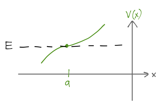
If we make the (usually justified) assumption that the function V(x) - E has a single zero at a, then a Taylor expansion gives V(x) - E \approx C(x-a) and the Schrödinger equation becomes -\frac{\hbar^2}{2m} \frac{d^2 u_E}{dx^2} + C(x-a) u_E(x) = 0.
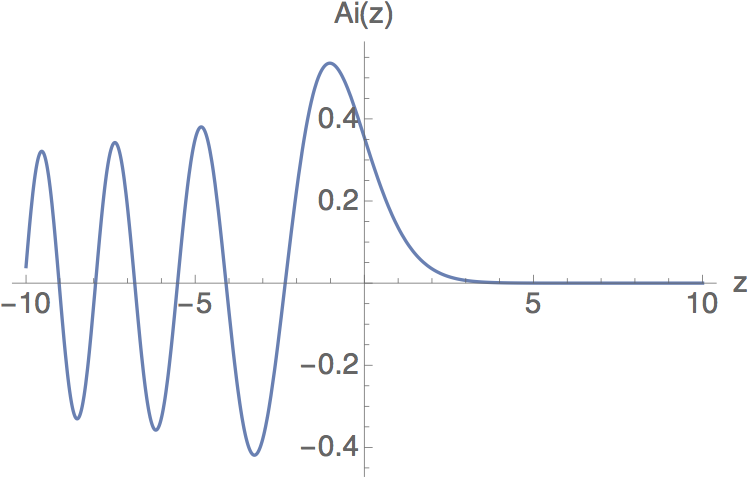
Transforming to A = 2mC / \hbar^2 and then z = A^{1/3} (x-a), the equation simplifies to \frac{d^2 u_E}{dz^2} - zu_E(z) = 0. This is now in standard form for a well-known differential equation, known as the Airy equation; its solutions are the Airy functions {\rm Ai}(z). The Airy function has an interesting functional form: for z < 0\ it oscillates somewhat like a plane wave, while for z > 0\ it is damped to zero somewhat like a pure exponential. Since the classical turning point is exactly where the energy crosses the potential barrier, this is exactly the behavior we expect.
In fact, as a second-order equation it should have two solutions; there is a second set of Airy functions denoted {\rm Bi}(z). You can probably guess that these also look like oscillatory solutions going over to exponential; the important difference is that {\rm Bi}(z) goes to infinity as z \rightarrow \infty, i.e. it acts like a growing exponential in the forbidden region. In some cases this may not be normalizable, but for the moment we’re working out generic forms for the connection formulas; whether certain real exponential solutions are discarded will depend on the problem we’re solving.
Since we are trying to join together WKB solutions on either side of a turning point, we expect to transition from oscillatory behavior to exponential growth and decay, or vice-versa; the Airy functions do precisely this, smoothly interpolating from one to the other. In fact, the asymptotic forms of the Airy functions are well known: (z \rightarrow +\infty): {\rm Ai}(z) \rightarrow \frac{1}{2\sqrt{\pi}} z^{-1/4} \exp \left( -\frac{2}{3} z^{3/2} \right) \\ (z \rightarrow -\infty): {\rm Ai}(z) \rightarrow \frac{1}{\sqrt{\pi}} |z|^{-1/4} \cos \left( \frac{2}{3} |z|^{3/2} - \frac{\pi}{4} \right). \\ For the other Airy function (Airy function of the second kind), we have similarly (z \rightarrow +\infty): {\rm Bi}(z) \rightarrow \frac{1}{\sqrt{\pi}} z^{-1/4} \exp \left( \frac{2}{3} z^{3/2} \right) \\ (z \rightarrow -\infty): {\rm Bi}(z) \rightarrow -\frac{1}{\sqrt{\pi}} |z|^{-1/4} \sin \left( \frac{2}{3} |z|^{3/2} - \frac{\pi}{4} \right). \\
These asymptotic forms are precisely what the WKB solutions look like (even down to the z^{-1/4} \sim 1/\sqrt{k}.) Matching the WKB solutions onto the joining functions at the boundaries gives rise to a set of “connection formulas”, which work just like any other set of boundary conditions, allowing us to determine the arbitrary constants in our general solution.
I’ll skip the details of the derivation, and just give you the results for the connection formulas.
If we have a potential V(x) with a classical turning point at x=a, and assume that V'(a) > 0, then if for x > a we have the general WKB solution \frac{A}{\sqrt{\kappa(x)}} \exp \left[ -\int_a^x dx'\ \kappa(x') \right] + \frac{B}{\sqrt{\kappa(x)}} \exp \left[ \int_a^x dx'\ \kappa(x') \right], then the solution for x < a takes the form \frac{2A}{\sqrt{k(x)}} \cos \left[ \int_x^a dx' k(x') - \frac{\pi}{4} \right] - \frac{B}{\sqrt{k(x)}} \sin \left[ \int_x^a dx' k(x') - \frac{\pi}{4} \right].
If instead the potential is decreasing at a, then we have exponentials on the left and oscillation on the right. The connection formulas are exactly the same, but with the replacement x-a \rightarrow a-x (which just flips the limits of integration upside down everywhere.)
Note the details that come from the asymptotic forms of the Airy functions: the factor of 2 on A, the phase shift of -\pi/4, and the minus sign on the \sin term.
Now, a natural question is whether it’s consistent to assume that the asymptotic forms are good replacements when we’re doing WKB, or whether this is secretly an additional assumption. Recall that the condition for WKB to work is |k'(x)| \ll |k^2(x)|. As we just showed, in the vicinity of a linear potential region, i.e. if V(x) - E \approx C(x-a) where C is a constant, the solutions to the Schrödinger equation become proportional to {\rm Ai}(z), where z is the dimensionless combination z = \left( \frac{2mC}{\hbar^2} \right)^{1/3} (x-a). In the process of solving for the wavefunction, it’s easy to see that k^2 \propto -z, so the WKB condition becomes (roughly) |z| \gg 1. This is good enough for us to use the asymptotic forms: numerically, the Airy functions become very close to their approximations around |z| \sim 3 or so. (The asymptotic forms actually diverge at z=0, whereas the real Airy functions don’t; but we’re only using them to connect between asymptotic regions, so we don’t care what happens at z=0.) I skipped quickly through details here; the full discussion can be found in Merzbacher 7.2.
Here, you should complete Tutorial 9 on “WKB connection formulas”. (Tutorials are not included with these lecture notes; if you’re in the class, you will find them on Canvas.)
19.3 Some WKB applications
Now that we have completed the formalism, let’s go through a couple of useful applications of WKB.
19.3.1 WKB and bound states
Suppose we have a potential well with some shape, and consider a bound state with energy such that the turning points are at x=a and x=b. We can divide the potential into three regions:
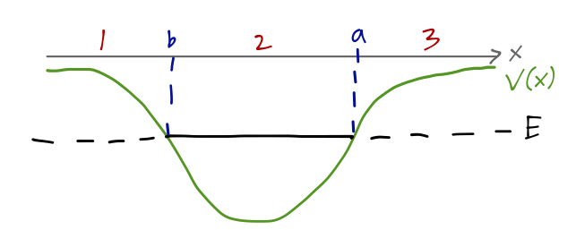
These are backwards from the natural order so that turning point a matches the derivation that we just finished. We’ll start in region 3 on the far right, where are usual the condition that the wavefunction can’t blow up as x \rightarrow \infty excludes one of the two possible exponential solutions, i.e. we have \psi_3(x) \approx \frac{A}{\sqrt{\kappa(x)}} \exp \left[- \int_a^x dx'\ \kappa(x') \right]. Now to find the solution in the middle region, we apply the WKB connection formula: reading off from above, we have \psi_2(x) \approx \frac{2A}{\sqrt{k(x)}} \cos \left[ \int_x^a dx'\ k(x') - \frac{\pi}{4} \right]. This is the full (approximation) wavefunction, but if we’d like to match across the other boundary at x=b, we need to rewrite it to shift the limits of integration accordingly. Since V(x) has the opposite slope there, we want the integrations to run from b to x. Since \int_x^a dx' k(x') + \int_b^x dx' k(x') = \int_b^a dx' k(x') \equiv C (defining the constant C given by integrating over the entire well), we have \psi_2(x) \approx \frac{2A}{\sqrt{k(x)}} \cos \left[ \int_b^a dx'\ k(x') - \int_b^x dx'\ k(x') - \frac{\pi}{4} \right] \\ = \frac{2A}{\sqrt{k(x)}} \left( \cos (C) \cos \left[ \int_b^x dx'\ k(x') + \frac{\pi}{4} \right] \right. \\ +\left. \sin (C) \sin \left[ \int_b^x dx'\ k(x') + \frac{\pi}{4} \right] \right) using an angle-addition formula; note that the integrals from a to b just give us constants that multiply the two x-dependent terms. To use the connection formulas we have to shift the phases inside by -\pi/2, which takes \sin \rightarrow \cos and \cos \rightarrow -\sin, leaving us with \psi_2(x) = \frac{2A}{\sqrt{k(x)}} \left( \sin(C) \cos \left[ \int_b^x dx' k(x') - \frac{\pi}{4} \right] -\cos(C) \sin \left[\int_b^x dx' k(x') - \frac{\pi}{4} \right] \right). This is now in the standard form for the connection formula at the left turning point x=b, which will give us the wavefunction in region 1: \psi_1(x) = \frac{A \sin(C) }{\sqrt{\kappa(x)}} \exp \left[ -\int_x^b dx' \kappa(x') \right] + \frac{2A \cos (C)}{\sqrt{\kappa(x)}} \exp \left[ \int_x^b dx' \kappa(x') \right]. But now we are once again in a region where there should be only one exponential solution, the one which dies off as x \rightarrow -\infty, since the other exponential won’t be normalizable. If we were dealing with free solutions then we would discard e^{-\kappa x}, which diverges as x \rightarrow -\infty. But in this case, we keep the first term with the minus sign in front, since the integral from -x to b is always positive. This means that the other coefficient must vanish: \cos(C) = \cos \left[ \int_b^a dx'\ k(x') \right] = 0, or \int_b^a dx'\ k(x') = \left(n + \frac{1}{2}\right) \pi, or \int_b^a \sqrt{2m(E-V(x))} = \pi \hbar \left(n + \frac{1}{2} \right). So long as the WKB approximation works well for our chosen potential (which primarily means that the turning points a and b must be separated by many wavelengths), this formula tells us what the bound-state energies can be.
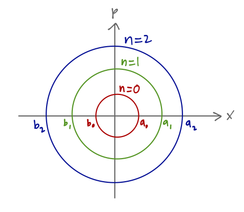
We should note that the quantity we are integrating over on the left-hand side is exactly the momentum, p(x) = \hbar k(x). Furthermore, the two points a and b are the classical turning points; a classical particle with energy E would move in an “orbit” between x=a and x=b. We can thus rewrite the integral in a more classical way, as an integral over the phase-space trajectory of our particle, \oint p(x) dx = h \left(n + \frac{1}{2} \right) where now we’ve recovered the un-barred Planck constant. (Note that we picked up a 2 since the phase-space integral goes around a complete circle, so it’s double the integral we started with.) Except for the shift by 1/2, this is exactly the Bohr-Sommerfeld quantization rule which was one of the foundations of the “old quantum” theory. Whereas a classical particle could have any bound-state energy E, the quantization rule allows only bound states for which the above action integral gives integer multiples of h.
19.3.2 WKB and quantum tunneling
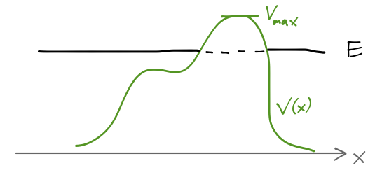
We can also gain some very useful insights from WKB in the case that we have a potential barrier, rather than a well. Again, we assume an arbitrary shape for V(x), but with slow enough variation that WKB can be applied, and we consider E < V_{\rm max} so that the particle cannot pass though the barrier classically.
As with the example of the square potential barrier, we can start by writing down our arbitrary solution in the three regions defined by the turning points a and b: \psi(x) = \begin{cases} \frac{A}{\sqrt{k(x)}} \exp \left[i \int_a^x dx' k(x') \right] + \frac{B}{\sqrt{k(x)}} \exp \left[ -i \int_a^x dx' k(x') \right], & (x < a); \\ \frac{C}{\sqrt{\kappa(x)}} \exp \left[- \int_a^x dx' \kappa(x') \right] + \frac{D}{\sqrt{\kappa(x)}} \exp \left[ \int_a^x dx' \kappa(x') \right], & (a < x < b); \\ \frac{F}{\sqrt{k(x)}} \exp \left[i \int_b^x dx' k(x') \right] + \frac{G}{\sqrt{k(x)}} \exp \left[ -i \int_b^x dx' k(x') \right], & (x > b). \\ \end{cases} With the connection formulas in hand, we can easily find the relationship between these coefficients. In fact, the result turns out to be quite simple: in matrix form, we find that \left( \begin{array}{c} A \\ B \end{array} \right) = \frac{1}{2} \left( \begin{array}{cc} 2\theta + \frac{1}{2\theta} & i (2\theta - \frac{1}{2\theta}) \\ -i(2\theta - \frac{1}{2\theta}) & 2\theta + \frac{1}{2\theta} \end{array} \right) \left( \begin{array}{c} F \\ G \end{array} \right) where \theta = \exp \left[ \int_a^b dx' \kappa(x') \right].
Derive the result above relating A and B to F and G. (Hint: this is just a longer version of what we did for bound states above - applying WKB connection at the turning points and then converting the integrals from one turning point to the next.)
Answer:
To apply the connection formulas, we need to convert from the “plane-wave” complex exponential form which is most useful for talking about reflection and transmission into sine and cosine with the appropriate phase shifts. Part of this conversion involves flipping the integrals upside down; integrating from a to x makes sense in terms of matching on to our standard plane-wave interpretations, but the connection formula at a wants the opposite.
Let’s go through the conversion: \frac{A}{\sqrt{k(x)}} \exp \left[i \int_a^x dx' k(x') \right] + \frac{B}{\sqrt{k(x)}} \exp \left[ -i \int_a^x dx' k(x') \right] \\ = \frac{Ae^{-i\pi/4}}{\sqrt{k(x)}} \exp \left[ -i \int_x^a dx' k(x') + \frac{i\pi}{4} \right] + \frac{Be^{+i\pi/4}}{\sqrt{k(x)}} \exp \left[ i \int_x^a dx' k(x') - \frac{i\pi}{4} \right] \\ = \frac{Ae^{-i\pi/4} + Be^{+i\pi/4}}{\sqrt{k(x)}} \cos \left[ \int_x^a dx' k(x') - \frac{\pi}{4} \right] + \frac{-iAe^{-i\pi/4} + iBe^{+i\pi/4}}{\sqrt{k(x)}} \sin \left[ \int_x^a dx' k(x') - \frac{\pi}{4} \right] Now applying the connection formulas, we find the relations C = \frac{Ae^{-i\pi/4} + Be^{+i\pi/4}}{2}, \\ D = iAe^{-i\pi/4} - iBe^{+i\pi/4}. We could now try to translate forwards to the turning point at x=b using these coefficients, but instead let’s just go to the third region and work backwards. We need to do the same translation on the right into a form useful for the connection formulas: \frac{F}{\sqrt{k(x)}} \exp \left[i \int_b^x dx' k(x') \right] + \frac{G}{\sqrt{k(x)}} \exp \left[ -i \int_b^x dx' k(x') \right] \\ = \frac{Fe^{+i\pi/4}}{\sqrt{k(x)}} \exp \left[ i \int_b^x dx' k(x') - \frac{i\pi}{4} \right] + \frac{Ge^{-i\pi/4}}{\sqrt{k(x)}} \exp \left[ -i \int_b^x dx' k(x') + \frac{i\pi}{4} \right] \\ = \frac{Fe^{+i\pi/4} + Ge^{-i\pi/4}}{\sqrt{k(x)}} \cos \left[ \int_b^x dx' k(x') - \frac{\pi}{4} \right] + \frac{iFe^{+i\pi/4} - iGe^{-i\pi/4}}{\sqrt{k(x)}} \sin \left[ \int_b^x dx' k(x') - \frac{\pi}{4} \right] We can use the connection formulas at this point, but the problem is that the functional form we connect onto is slightly different from how we wrote things above. If we write \frac{C'}{\sqrt{\kappa(x)}} \exp \left[ -\int_x^b dx' \kappa(x')\right] + \frac{D'}{\sqrt{\kappa(x)}} \exp \left[ \int_x^b dx' \kappa(x') \right] then the connection formulas give us C' = \frac{Fe^{+i\pi/4} + Ge^{-i\pi/4}}{2} \\ D' = -iFe^{+i\pi/4} + iGe^{-i\pi/4}.
Now we need to figure out how C',D' are related to C,D, which is how the integral that gives \theta is going to appear. First, C \exp \left[ -\int_a^x dx' \kappa(x') \right] = C \exp \left[ -\int_a^b dx' \kappa(x') + \int_x^b dx' \kappa(x') \right] = \frac{C}{\theta} \exp \left[ \int_x^b dx' \kappa(x') \right] so D' = C/\theta. Similarly, we find D \exp \left[ \int_a^x dx' \kappa(x') \right] = D \exp \left[ \int_a^b dx' \kappa(x') - \int_x^b dx' \kappa(x') \right] = D \theta \exp \left[ -\int_x^b dx' \kappa(x') \right], telling us that C' = D\theta. Putting things together, we have the system of equations
C' = D\theta \Rightarrow Fe^{i\pi/4} + Ge^{-i\pi/4} = 2iA\theta e^{-i\pi/4} - 2iB\theta e^{+i\pi/4} \\ D' = C/\theta \Rightarrow -2iF e^{i\pi/4} + 2iG e^{-i\pi/4} = \frac{A}{\theta} e^{-i\pi/4} + \frac{B}{\theta} e^{+i\pi/4} To match the given form of a matrix equation, we want to isolate A and B. First multiplying through by e^{i\pi/4} and moving some terms around, iF/\theta + G/\theta = 2iA + 2B \\ 2F\theta + 2iG\theta = A + iB Adding 2i times the second equation to the first gives iF (1/\theta + 4\theta) + G(1/\theta - 4\theta) = 4iA \\ \Rightarrow A = \frac{F}{2} \left(2\theta + \frac{1}{2\theta} \right) + \frac{iG}{2} \left( 2\theta - \frac{1}{2\theta} \right) and subtracting 2i instead leads to iF (1/\theta - 4\theta) + G(1/\theta + 4\theta) = 4B \\ \Rightarrow B = \frac{-iF}{2} \left( 2\theta - \frac{1}{2\theta} \right) + \frac{G}{2} \left( 2\theta + \frac{1}{2\theta} \right).
Reading off from these equations, we find the matrix-form solution exactly as written above.
So as far as the transmission and reflection of incoming waves are concerned, all of the information about the barrier is encoded in the single integral which gives \theta. We can read off the transmission coefficient from this matrix, T = \frac{|F|^2}{|A|^2} = \frac{4}{\left(2\theta + \frac{1}{2\theta}\right)^2}. In the limit that the barrier is high and wide, then \theta becomes large, and we simply have T \approx \frac{1}{\theta^2} = \exp \left[ -2 \int_a^b dx'\ \kappa(x') \right] = \exp \left[ -\frac{2}{\hbar} \int_a^b \sqrt{2m(V(x)-E)} \right].
An early quantum-mechanical model of nuclear \alpha decay is given by the Gamow-Gurney-Condon theory (see here for a historical review), which treats it entirely as a tunneling process. Roughly, the model treats the \alpha particle (which is a helium-4 nucleus) as a single object which is bound in a deep, square potential well of width R, corresponding to the radius of the parent nucleus. Once the \alpha particle escapes, it will be repelled by the Coulomb force. So the overall potential looks like this:
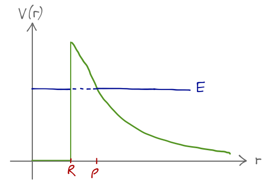
V(x) = \begin{cases} 0, & 0 < r < R;\\ \frac{2Ze^2}{r}, & r > R. \end{cases} where Z is the charge of the daughter nucleus in the decay. Ignoring the fact that the potential step at R is pretty sharp and not WKB friendly at all (we’ll take the size R to be very small anyway, the interesting physics comes from the Coulomb barrier), we can calculate the transmission coefficient in the approximation of a large barrier: -\frac{1}{2} \log T = \int_R^\rho dr'\ \kappa(r') = \frac{\sqrt{2m}}{\hbar} \int_R^\rho dr' \sqrt{\frac{2Ze^2}{r'} - E}. Note that there is not a factor of r'{}^2 as we would normally expect for a three-dimensional problem in spherical coordinates, which is what we need to describe real-world alpha decays. I won’t go into any details on the three-dimensional version of WKB, but the upshot for present purposes is that if you go through the derivation for the radial Schrödinger equation, the result is exactly the same as the one-dimensional version - an integral over the wave number, without any extra factors.
The position \rho of the second turning point is given by the condition E = 2Ze^2/\rho. If we take E = \frac{1}{2} mv^2 using the speed of the escaping alpha, then in the limit R \rightarrow 0 the integral yields the result -\frac{1}{2} \log T \approx \frac{2\pi Z e^2}{\hbar v} or T \approx \exp \left[ -\frac{4\pi Z e^2}{\hbar v}\right]. (If you do the integral properly in Mathematica, you can find a full expression including the R dependence.) The striking feature here is that the transmission probability is exponentially sensitive to the nuclear charge, Z. We can turn this transmission coefficient into a decay rate: if on average the alpha particle strikes the barrier inside the nucleus with a frequency of v/(2R), then the decay rate should be \lambda = \frac{Tv}{2R}. This formula (or more accurately, the full expression with the R values included) does an excellent job of reproducing experimental data for alpha decay spanning 23 orders of magnitude in lifetime!