22 A deep dive into hydrogen
Although the “hydrogen atom” as you learn it in class is a nice, simple, exactly solvable quantum system, it has one drawback; the simple model doesn’t completely describe the real hydrogen atom. There are a number of physical effects which give small corrections to the exact solutions; these corrections are known as the fine (small) and hyperfine (really small) structure of the hydrogen atom. We’ve seen bits and pieces of these corrections before, but now that we’ve developed perturbation theory, we’re ready to tackle them systematically.
Actually, most of the effects we’re about to study in perturbation theory secretly come from relativistic corrections in one way or another. There is an exact solution which incorporates many of the fine and hyperfine corrections, but it requires a relativistic formulation of quantum mechanics using the Dirac equation, which is not currently covered in these notes. Even the Dirac solution is missing some effects, such as corrections due to nuclear size and spin, that can sometimes matter; and of course, for anything beyond hydrogen we need perturbation theory or other methods anyway.
For the most part, here we will work with Z=1, specializing to the hydrogen atom and not just single-electron (“hydrogenic”) atoms. For atoms with larger Z there are other corrections which can change the relative magnitude of these terms or introduce new effects to deal with. In some places in the derivations below I will include explicit Z factors and comment on other atoms. We will have to include the spin of the electron in our calculations now, so we label the hydrogen eigenstates as \ket{n, l, m, m_s}.
We’ll begin with the fine structure. There are three terms we must consider, which give rise to corrections of roughly the same magnitude: \hat{H}_{\rm fine} = \hat{H}_0 + \hat{W}_{rel} + \hat{W}_{SO} + \hat{W}_D. \hat{H}_0 here is the kinetic term and the Coulomb interaction. The three terms, in order, are known as the relativistic correction to the kinetic energy, the spin-orbit coupling, and the Darwin term. Let’s have a closer look at each of them. As we will see explicitly, each of these terms is of order \alpha^2, where \alpha = e^2 / (\hbar c) is the fine-structure constant; so to work consistently in perturbation theory, we need to include all three at once.
As a reminder and point of reference, key combinations of physical units relevant for hydrogen are the Bohr radius, a_0 = \frac{\hbar^2}{m_e e^2}, and the fine-structure constant, \alpha = \frac{e^2}{\hbar c}. The ground-state energy of the unperturbed solution \hat{H}_0 is E_{100}^{(0)} = -\frac{m_e e^4}{2\hbar^2} = -\frac{e^2}{2a_0} = -\frac{1}{2} m_e c^2 \alpha^2 = -1\ \textrm{Ry}, defining the Rydberg (1 Ry = 13.6 eV) as a baseline unit of energy; other states \ket{nlm} have energies of 1/n^2\ \textrm{Ry}. All energies are multiplied by Z^2 for a hydrogenic atom with Z>1.
22.1 Relativistic correction to kinetic energy
The kinetic energy term T = \frac{p^2}{2m} is only correct non-relativistically; we know that the true kinetic energy of a relativistic particle is T = \sqrt{p^2 c^2 + m^2 c^4} - mc^2.
Why should we need to consider such a relativistic effect? Is the orbital electron in a hydrogen atom really moving at relativistic speeds? We could answer this in something like the Bohr model, but in quantum mechanics the question seems slightly ill-posed: an electron in the 1s energy eigenstate is in a quantum state that doesn’t evolve in time, so how do we think about “motion”?
The least confusing thing we can do is talk about momentum instead of speed, since that is well-defined through the Hamiltonian: the average electron speed can be characterized by \bar{v} \equiv \sqrt{\left\langle \hat{p}^2 \right\rangle} / m_e. (We have to use the squared momentum operator since the expectation of the vector \hat{\vec{p}} is generally zero by symmetry.) Since we’re talking about modifying the kinetic term, the size of expectation values of momentum is what is relevant to the size of the perturbation anyway. Let’s calculate this for the ground state:
\left\langle \hat{p}^2 \right\rangle = \int_0^\infty dr\ r^2 4 \frac{Z^3}{a_0^3} e^{-Zr/a_0} \left( -\hbar^2 \nabla^2 \right) e^{-Zr/a_0} \\ = \frac{-4\hbar^2 Z^3}{a_0^3} \int_0^\infty dr\ e^{-Zr/a_0} \frac{\partial}{\partial r} \left( r^2 \frac{\partial}{\partial r} e^{-Zr/a_0} \right) \\ = \frac{4\hbar^2 Z^4}{a_0^4} \int_0^\infty dr\ e^{-Zr/a_0} \left( 2r e^{-Zr/a_0} - \frac{Zr^2}{a_0} e^{-Zr/a_0} \right) \\ = \frac{4\hbar^2 Z^4}{a_0^4} \left(\frac{a_0^2}{4Z^2}\right) = \frac{\hbar^2 Z^2}{a_0^2} so \bar{v} = Z \hbar / (m_e a_0) = \frac{Z \hbar}{m_e} \frac{m_e e^2}{\hbar^2} = \frac{Ze^2}{\hbar} = Z \alpha c. In other words, for the hydrogen atom with Z=1, the speed of the electron is v/c \sim \alpha \sim 1/137. This is much smaller than the speed of light, but large enough that relativistic corrections will still be noticeable.
This result was just for the ground state, but we expect excited states to have lower electron speeds, since the orbitals are larger (and anyway, we’ll verify the size of the perturbation when we calculate it in full below.)
Knowing that the speed of the electron is relatively small in the hydrogen atom, we can deal with it by expanding the kinetic energy as a series in p: T \approx \frac{p^2}{2m_e} - \frac{p^4}{8m_e^3c^2} + ... and treating the new term as a perturbation, so \hat{W}_{rel} = -\frac{\hat{p}^4}{8m_e^3 c^2}. This is a degenerate-state perturbation theory problem, since the hydrogen states have degeneracy n^2. However, for this particular perturbation we can easily see that [\hat{\vec{L}}, \hat{W}_{rel}] = 0 (and thus [\hat{L}{}^2, \hat{W}_{rel}] = 0 as well), which means that as long as we work in the angular momentum eigenbasis \ket{nlm}, the perturbation is diagonal and all ambiguities are removed. So we can proceed to calculating the first-order energy shift as the usual expectation value, E_{nl}^{(1)} = \bra{nlm} \hat{W}_{rel} \ket{nlm} = -\frac{1}{8m_e^3 c^2} \left\langle (\hat{p}{}^2)^2 \right\rangle. It’s possible to evaluate the expectation value by brute force, particularly if we’re given a particular \ket{nlm} state, but some tricky rewriting will let us quickly find the right answer. Since the Hamiltonian contains two terms, the \hat{p}^2 kinetic term and the 1/r Coulomb potential, we can trade one for the other: \left\langle \hat{W}_{rel} \right\rangle = -\frac{1}{2m_e c^2} \left\langle \left( \frac{\hat{p}^2}{2m_e}\right)^2 \right\rangle \\ = -\frac{1}{2m_e c^2} \left\langle \left( \hat{H}_0 + \frac{Ze^2}{r} \right)^2 \right\rangle \\ = -\frac{1}{2m_e c^2} \left( (E_n^{(0)})^2 + 2E_n^{(0)} Ze^2 \left\langle \frac{1}{r} \right\rangle + Z^2 e^4 \left\langle \frac{1}{r^2} \right\rangle \right). The first expectation value \left\langle 1/r \right\rangle is easy to calculate. Remember that the virial theorem relates the expectation values of kinetic and potential energy, 2\left\langle T \right\rangle = -\left\langle V \right\rangle. But we also know that \left\langle T \right\rangle = \left\langle H \right\rangle - \left\langle V \right\rangle = E_n^{(0)} - \left\langle V \right\rangle, so \left\langle V \right\rangle = 2E_n^{(0)}, i.e. \left\langle \frac{1}{r} \right\rangle = \frac{-2E_n^{(0)}}{Ze^2}.
22.1.1 The Feynman-Hellmann theorem
Let’s take a quick detour to derive a very useful little theorem, called the Feynman-Hellmann theorem. The theorem allows us to calculate expectation values by taking derivatives of energy eigenvalues.
Given a quantum system with Hamiltonian \hat{H} that depends on some parameter \lambda, the derivative of the energy with respect to \lambda is related to a matrix element of the derivative of \hat{H},
\frac{dE_\lambda}{d\lambda} = \bra{E_{\lambda}} \frac{d\hat{H}}{d\lambda} \ket{E_{\lambda}}.
To derive this result, we start by observing that E_\lambda = \bra{E_{\lambda}} \hat{H}_{\lambda} \ket{E_{\lambda}} and then differentiating both sides: \frac{dE_{\lambda}}{d\lambda} = \left( \frac{d}{d\lambda} \bra{E_{\lambda}}\right) \hat{H}_{\lambda} \ket{E_{\lambda}} + \bra{E_{\lambda}} \frac{d\hat{H}_{\lambda}}{d\lambda} \ket{E_{\lambda}} + \bra{E_{\lambda}} \hat{H}_{\lambda} \left( \frac{d}{d\lambda} \ket{E_{\lambda}} \right). In the first and third terms, we can act \hat{H}_{\lambda} on the energy eigenstates and pull out E_{\lambda}: \frac{dE_{\lambda}}{d\lambda} = \bra{E_{\lambda}} \frac{d\hat{H}_{\lambda}}{d\lambda} \ket{E_{\lambda}} + E_{\lambda} \left[ \left( \frac{d}{d\lambda} \bra{E_{\lambda}} \right) \ket{E_{\lambda}} + \bra{E_{\lambda}} \left( \frac{d}{d\lambda} \ket{E_{\lambda}} \right) \right] \\ = \bra{E_{\lambda}} \frac{d\hat{H}_{\lambda}}{d\lambda} \ket{E_{\lambda}} + E_{\lambda} \frac{d}{d\lambda} (\left\langle E_{\lambda} | E_{\lambda} \right\rangle). But the inner product of the state with itself \left\langle E_\lambda | E_\lambda \right\rangle = 1, so the last term vanishes, and we have proven the theorem.
The Feynman-Hellmann theorem is a simple but powerful result for evaluating certain expectation values. To apply it to the hydrogen atom, let’s write out the unperturbed Hamiltonian in position space: \hat{H}_0 = \frac{\hat{p}^2}{2m_e} - \frac{Ze^2}{\hat{r}} \\ \Rightarrow \bra{\hat{\vec{r}}} \hat{H} \ket{nlm} = -\frac{\hbar^2}{2m_er^2} \left[ \frac{d}{dr} \left( r^2 \frac{d}{dr} \right) - l(l+1) \right] \psi_{nlm}(r) - \frac{Ze^2}{r} \psi_{nlm}(r). Now, here’s the tricky part. The Feynman-Hellmann theorem is a purely mathematical statement about the expectation values; it essentially doesn’t “know about” the physics. In particular, it is perfectly valid to apply it to the angular momentum eigenvalue l: \frac{dE_{nlm}^{(0)}}{dl} = \bra{nlm} \frac{d\hat{H}_0}{dl} \ket{nlm} \\ = \frac{\hbar^2 (2l+1)}{2m_e} \left\langle \frac{1}{r^2} \right\rangle. Again, we can differentiate like this even though we know that only integer values of l are physical; we’re making a purely mathematical statement.
What about the left-hand side? As we know, the energies depend solely on the value of principal quantum number n: E_{nlm}^{(0)} = -\frac{Z^2}{n^2}\ \textrm{Ry} = -\frac{Z^2 e^2}{2a_0 n^2}. This looks independent of l, and in fact we’ve emphasized that for a given value of n, the corresponding angular momentum levels are degenerate. However, mathematically we remember that n is a just a convenient rewriting of the true radial and angular quantum numbers, n = q + l + 1. So \frac{dE_{nlm}^{(0)}}{dl} = \frac{dE_{nlm}}{dn} = \frac{Z^2 e^2}{a_0 n^3}. Substituting back in, we find that \left\langle \frac{1}{r^2} \right\rangle = \frac{2m_e Z^2 e^2}{a_0 \hbar^2 n^3 (2l+1)} \\ = \frac{1}{a_0^2 n^3 (l+1/2)}, recalling the definition of the Bohr radius a_0 = \hbar^2 / m_e e^2. Notice that we could also have found \left\langle 1/r \right\rangle through the Feynman-Hellmann theorem, by applying it to the electric charge; it’s worth going through the exercise at home if you’re still uncertain about this derivation.
Finally, back to the relativistic correction: we now have \left\langle \hat{W}_{rel} \right\rangle = -\frac{1}{2m_e c^2} \left( -3 (E_n^{(0)})^2 + Z^4 e^4 \left( \frac{1}{a_0^2 n^3 (l+1/2)}\right) \right) \\ = -\frac{Z^4 e^4}{2m_e c^2 n^3} \left( \frac{-3}{4 n a_0^2} + \frac{1}{a_0^2 (l+1/2)} \right) \\ = \frac{Z^4 e^2}{m_e c^2 n^3 a_0} \left( \frac{3}{4n} - \frac{1}{l+1/2} \right)\ \textrm{Ry} Let’s try to combine some of the parameters out front, with a preference for dimensionless numbers like \alpha. We can see that \frac{e^2}{m_e c^2 a_0} = \frac{e^4}{\hbar^2 c^2} = \alpha^2, so finally, the relativistic energy shift at first order is \Delta_n^{(1)} = \frac{Z^4 \alpha^2}{n^3} \left[ \frac{3}{4n} - \frac{1}{l+1/2} \right]\ \textrm{Ry}. Since the ground-state energy itself scales as Z^2, we see that the relative correction here is on the order of Z^2 \alpha^2. For hydrogen itself this is on the order of a part per ten thousand, which is quite small; it is one of the many terms that make up the so-called “hyperfine corrections” to the spectrum of hydrogen. Clearly for larger nuclei, the relativistic shift will be more significant; the stronger Coulomb potential for larger Z pulls in the electron orbits and gives them a higher average speed.
On the other hand, we see that as expected, the correction is smaller for orbitals with larger n (the average speed is lower for orbitals that are more extended.) We can also note that since for hydrogen we must have l < n, the sign of the correction is always negative, as it must be since \hat{W} \sim -\left\langle \hat{p}^4 \right\rangle is negative definite.
22.2 Spin-orbit coupling
The second term is the spin-orbit coupling, \hat{W}_{SO} = \frac{e^2}{2m_e^2 c^2 r^3} \hat{\vec{L}} \cdot \hat{\vec{S}} Physically, this term arises from the interaction of the electron’s magnetic moment with the magnetic field which the electron “sees” due to its motion through the proton’s static electric field. (As you know from E&M, this is again a relativistic correction.)
We have studied this interaction before, when considering addition of angular momentum. We rewrote this in terms of the total angular momentum \hat{\vec{J}} = \hat{\vec{L}} + \hat{\vec{S}}, \hat{\vec{L}} \cdot \hat{\vec{S}} = \frac{1}{2} \left( \hat{J}^2 - \hat{L}^2 - \hat{S}^2 \right). We advertised this rewriting as a convenient change of basis before, but it’s actually necessary in the context of perturbation theory, to avoid running into the degenerate state problem; working in the \hat{\vec{J}} eigenbasis diagonalizes the spin-orbit term.
Relative to the Coulomb potential e^2 / r, the size of the spin-orbit term can be written \frac{W_{SO}}{V_0} = \frac{\hbar^2}{m_e^2 c^2 r^2} \sim \frac{\hbar^2}{m_e^2 c^2 a_0^2} = \alpha^2, where we’re making a rough approximation by assuming that r is most probably the Bohr radius a_0. This leads to another result proportional to \alpha^2, like the relativistic correction.
To deal with this perturbation we already know that it will be simplest to work in the \ket{nljm} total angular momentum eigenbasis, in which case we can write out the desired expectation value as \bra{jm} \hat{\vec{L}} \cdot \hat{\vec{S}} \ket{jm} = \bra{jm} \frac{1}{2} (\hat{\vec{J}}{}^2 - \hat{\vec{L}}{}^2 - \hat{\vec{S}}{}^2) \ket{jm} \\ = \frac{1}{2} \hbar^2 \left[ j(j+1) - l(l+1) - s(s+1) \right] This isn’t the whole story, however; this takes care of the angular dependence, but the spin-orbit coupling term also has a 1/r^3 radial dependence, so to actually compute the expectation value \left\langle \hat{\vec{L}} \cdot \hat{\vec{S}} \right\rangle, we need to evaluate a radial integral as well. Unlike the kinetic energy correction above, the Feynman-Hellmann theorem won’t help us to directly evaluate \left\langle 1/r^3 \right\rangle since there is no corresponding term in the Hamiltonian.
There does exist a recursion relation between expectation values of various powers of r in hydrogen, known as the Kramers relation, which can be used to obtain all such expectation values based on the ones we already know; this would allow us to write a formula for \left\langle 1/r^3 \right\rangle, but its derivation is tedious and the result is messy, so we’ll just stick with direct evaluation of radial integrals in these notes.
Now, we should worry a bit about degenerate states since we’re doing perturbation theory. In particular, we can see that this term (and the previous kinetic-energy term too, in fact) doesn’t depend on the magnetic quantum numbers m_l, m_s at all. Even in the total basis, it doesn’t depend on m, which means e.g. the three p-wave states \ket{l=1,m} are all degenerate.
The good news is that we’ve already solved this problem in the past! By going to the total angular momentum basis \ket{jm}, the perturbation \hat{W}_{so} is already fully diagonalized, so we don’t need to do anything else in order to proceed with our perturbative calculation.
22.3 Darwin term
The third term is known as the Darwin term, \hat{W}_D = -\frac{\hbar^2}{8m_e^2 c^2} \nabla^2 V(\hat{\vec{r}}) = \frac{\pi e^2 \hbar^2}{2m_e^2 c^2} \delta(\hat{\vec{r}}), since the Laplacian of the Coulomb 1/r potential is zero everywhere except the origin. This is a very mysterious-looking term, and it doesn’t really have a nice physical story unlike the previous two interactions. In fact, this term was first written down by Sir Charles Darwin (grandson of the other Darwin) after he solved the Dirac equation in full, and then discovered it in the non-relativistic expansion.
The Darwin term comes from the motion of the electron itself; there is really no good non-relativistic justification for it, in my opinion. It is a purely relativistic effect, which arises from the fact that a relativistic quantum particle with spin does not conserve orbital angular momentum when it moves; the result of this is that if we study the evolution of the position operator \hat{\vec{r}}(t), we will find a “jittering” of the motion about the classical path.
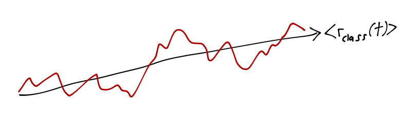
(Like many hard-to-understand physics concepts, this one has a fancy German word associated with it; the phenomenon is called zitterbewegung, or “trembling motion”.) This intrinsic uncertainty in the motion of the electron causes it to be sensitive to the potential V(r) non-locally when we expand non-relativistically, with the Darwin term proportional to \nabla^2 V(r) being the leading effect.
You can find some slightly more rigorous attempts to justify the Darwin term non-relativistically if you look through the literature; in my opinion, you won’t gain much from any of them. Understanding the Dirac equation itself is probably the best way you can feel better about the Darwin term, if you are so inclined.
We can see that the expectation value of the Darwin term will be zero unless we have \psi(0) \neq 0, which only holds for s orbitals; this correction is zero for higher values of l. For the s orbitals, we can see that \left\langle \hat{W}_D \right\rangle = \frac{\pi e^2 \hbar^2}{2m_e^2 c^2} |\psi(0)|^2. If you go back to the general formula for the hydrogen radial wavefunctions, you’ll find that they simplify drastically if l=0 and r=0; we find some terms depending on n, and then a factor of 1/\sqrt{\pi a_0^{3}}. (We could have guessed this from dimensional analysis, since we must have \int dr r^2 |R_{nl}(r)|^2 = 1.) Substituting in and simplifying, we find that since a_0^3 = \hbar^6 / m_e^3 e^6, \left\langle \hat{W}_D \right\rangle \sim m_e c^2 \frac{e^8}{\hbar^4 c^4} = m_e c^2 \alpha^4. (neglecting the n dependence and just looking at dimensions). This confirms that the Darwin term is of the same size as the other fine-structure contributions, i.e. it is of order \alpha^2 in Rydberg units.
22.4 Example: n=2 hydrogen fine structure
Now let’s return to an explicit study of the n=2 energy level of hydrogen, and work out all of the fine-structure corrections. Most of these corrections are not difficult to find for general n, but the number of states to deal with proliferates, so we’ll focus on n=2 to be concrete; our results here are easily extended to higher n.
We should begin by noting that none of the fine structure perturbations connect states with different l; this is an obvious statement for any energy level, not just n=2, since it’s easy to see that [\hat{L}^2, \hat{W}_{fine}] = 0.
Better yet, if we use the appropriate angular-momentum basis, the perturbation \hat{W}_{fine} is in fact automatically diagonal. For the kinetic energy correction and the Darwin term, this statement is fairly trivial; these operators are both scalars (rank-0 spherical tensors), so they only connect matrix elements with equal l, m, and m_s.
Let’s go through and calculate the explicit corrections.
22.4.0.1 Corrections to the 2s energy
We found above a general formula for the first-order energy correction due to the relativistic \hat{p}^4 kinetic term: \left\langle \hat{W}_{rel} \right\rangle = \frac{\alpha^2}{n^3} \left[ \frac{3}{4n} - \frac{1}{l+1/2} \right]\ \textrm{Ry} So for the 2s level, we have \left\langle \hat{W}_{rel} \right\rangle_{2s} = -\frac{13}{64}\ \alpha^2 \textrm{Ry} The Darwin term, which involves a delta function in position space, is non-zero here since \psi(0) \neq 0 in the s-wave. There’s no good trick to evaluate it, we simply have to plug in the explicit form of the wavefunction; we find after simplifying that \left\langle \hat{W}_D \right\rangle_{2s} = \frac{1}{8}\ \alpha^2 \textrm{Ry}
Derive the result above for \left\langle \hat{W}_D \right\rangle_{2s}.
Answer:
Detailed answer to be added!Finally, the spin-orbit term is zero in this state. Since l=0, the expectation value of \hat{\vec{L}} \cdot \hat{\vec{S}} is proportional to the matrix elements \bra{l=0,m=0} \hat{L}_{x,y,z} \ket{l=0,m=0} which uniformly vanish. Thus, \left\langle \hat{W}_{SO} \right\rangle_{2s} = 0.
22.4.0.2 Corrections to the 2p energy
This time, we’ll start with the Darwin term: since for any l>0 hydrogen state the wavefunction is zero at the origin, we have immediately \left\langle \hat{W}_D \right\rangle_{2p} = 0.
The kinetic energy correction is easy, we just have to plug in to our formula above once more: \left\langle \hat{W}_{rel} \right\rangle_{2p} = -\frac{7}{192}\ \alpha^2 \textrm{Ry}
That just leaves the spin-orbit coupling, which is now non-zero and requires slightly more effort to calculate. As we know, to deal with this perturbation we must work in the \ket{nljm} eigenbasis, the spin and angular momentum part gives us \bra{nljm} \hat{\vec{L}} \cdot \hat{\vec{S}} \ket{nljm} = \frac{1}{2} \hbar^2 \left[ j(j+1) - l(l+1) - s(s+1) \right] \\ = \begin{cases} -\hbar^2, & j=1/2; \\ +\hbar^2/2, & j=3/2. \end{cases} To get the full result, we add in the radial dependence. As discussed above, the general way to attack the resulting \left\langle 1/r^3 \right\rangle integral is messy, so here we just plug in the R_{21}(r) function explicitly (see the appendix on hydrogen) and do the integral. After the dust settles, you should find that \left\langle \hat{W}_{SO} \right\rangle = \frac{\alpha^2}{24 \hbar^2} \left\langle \hat{\vec{L}} \cdot \hat{\vec{S}} \right\rangle\ \textrm{Ry}, so plugging in the angular momentum values, we have finally \left\langle \hat{W}_{SO} \right\rangle_{2p,j=1/2} = -\frac{1}{24} \alpha^2\ \textrm{Ry}, \\ \left\langle \hat{W}_{SO} \right\rangle_{2p,j=3/2} = \frac{1}{48} \alpha^2\ \textrm{Ry}.
22.4.1 Combined results; the Lamb shift
We combine all of the above results to find the fine-structure corrections to the energy levels of n=2 hydrogen at leading order in \alpha: \Delta E_{2s} = \left( -\frac{13}{64} + \frac{8}{64} \right) \alpha^2\ \textrm{Ry} \\ = -\frac{5}{64}\alpha^2 \ \textrm{Ry}; \\ \Delta E_{2p,j=1/2} = \left( -\frac{7}{192} - \frac{8}{192} \right) \alpha^2\ \textrm{Ry} \\ = -\frac{5}{64}\alpha^2 \ \textrm{Ry}; \\ \Delta E_{2p,j=3/2} = \left( -\frac{7}{192} + \frac{4}{192} \right) \alpha^2\ \textrm{Ry} \\ = -\frac{1}{64} \alpha^2\ \textrm{Ry}.
Notice first of all that the splitting between the 2p energy levels is entirely determined by the spin-orbit coupling; the other effects don’t depend on the value of j.
A striking fact about these energy levels is that the 2s and 2p_{1/2} levels are degenerate, despite the fact that their energy corrections include contributions from seemingly different sources (the Darwin term vs. spin-orbit coupling)! This is sometimes called an “accidental” degeneracy, since there’s no apparent symmetry that forces the two levels to be equal.
However, the degeneracy isn’t really accidental. Remember that all of this fine structure comes from a non-relativistic expansion, and underlying it all is an exact relativistic solution using the Dirac equation. We won’t get to the equation itself, but the exact energy level is given by E_{\textrm{Dirac}} = m_e c^2 \left[ 1 + \alpha^2 \left(n - j - \frac{1}{2} + \sqrt{(j+1/2)^2 - \alpha^2} \right)^{-2} \right]^{-1/2} This reveals the reason for the degeneracy; energies in hydrogen from the Dirac equation depend on n and j, and the two levels which are degenerate here both have j = 1/2.
I should further note that despite our best efforts to be careful, we have not reproduced the experimental situation quite right; the 2s and 2p_{1/2} states are not degenerate in reality! There is one important effect which we have neglected, that we cannot deal with using our current framework, namely the quantum mechanical nature of the electromagnetic field itself. The missing effect gives rise to the Lamb shift, which is subleading to everything we’ve studied so far; it arises as an order \alpha^3 correction to the unperturbed energy level.
For these particular energy levels, the splitting corresponds to a frequency of 1060 MHz - to be compared to \sim 2000 THz from the difference between the n=2 and n=1 orbital energy levels, or 10 GHz for the fine splitting between 2p,j=1/2 and 2p,j=3/2 that we just found.
22.5 Hyperfine structure of hydrogen
In all of the above, we have been focused completely on the electron and have essentially ignored the proton itself as anything but a static charge. Since the proton is so much heavier than the electron, this is mostly a reasonable approximation. However, the proton is in fact a spin-1/2 particle like the electron, so we should account for its spin degree of freedom as well; this will lead to new magnetic effects.
As you saw on the homework, the spin of the proton is conventionally denoted by \hat{\vec{I}}. As with the electron, the proton’s spin has an associated magnetic moment, \hat{\mu}_I = \frac{g_p \mu_n}{\hbar} \hat{\vec{I}}. \mu_n is the “nuclear magneton”, \mu_n = \frac{e\hbar}{2m_p}, while g_p is the gyromagnetic ratio of the proton. For the electron, g_e \approx 2; the proton is a rather more complicated spin-1/2 object, and its g-factor is g_p \approx 5.6. Although the electron and proton carry the same angular momentum (eigenvalues \pm \hbar/2), the tiny size of the nuclear magneton relative to the Bohr magneton appearing in the spin-orbit interaction means that any effects due to nuclear spin will be further suppressed by m_e / m_p. These will all be \sim 2000 times smaller than the fine-structure terms, and are known as hyperfine corrections.
A careful study of the system leads to three terms once again at the hyperfine level: a spin-orbit coupling \hat{\mu}_I \cdot \hat{\vec{L}}, a direct coupling between the nuclear and electron spins \sim \hat{\mu}_I \cdot \hat{\vec{S}}, and a final spin-spin term containing a delta function, which is the hyperfine analogue of the Darwin term. I won’t go write the full hyperfine Hamiltonian out here, but you can find them in chapter 12 of Cohen-Tannoudji, among other places.
22.6 Example: n=1 hyperfine structure
Now we’ll briefly consider the hyperfine structure, this time moving back down to the n=1 energy level. The analysis is straightforward but much more complex for higher n states, and the hyperfine interactions will actually split the 1s state, unlike the fine-structure terms.
There is still a fine-structure correction to the 1s energy level, of course. You can verify easily that the values of the fine-structure terms are \left\langle \hat{W}_{rel} \right\rangle = -\frac{5}{8} \alpha^2\ \textrm{Ry}, \\ \left\langle \hat{W}_D \right\rangle = \frac{1}{2} \alpha^2\ \textrm{Ry}, and the spin-orbit term is again zero for an s orbital. Thus, the overall energy of the 1s level is shifted down by \Delta E_{1,f} = -\frac{1}{8} \alpha^2\ \textrm{Ry}. There is no splitting induced by this correction. Including the spin of the electron and now also of the proton, there are four degenerate states within the 1s level; we can write them in the basis \ket{s i; m_s m_i} suppressing the n and l labels which are constant here. Now, we consider the hyperfine interactions. As I noted before, two of the three interactions vanish for the 1s state; one is a spin-orbit type term which vanishes when l=0, and the other is a dipole-dipole interaction which vanishes due to the spherical symmetry of an s state. That just leaves us with the contact term. Plugging in the radial wavefunction |R_{10}(0)|^2, it’s easy to show that \left\langle \hat{W}_{hf,C} \right\rangle = \left(\frac{2}{3 \hbar^2} g_p \frac{m_e}{m_p} \left( 1 + \frac{m_e}{m_p}\right)^{-3} \alpha^2\ \textrm{Ry}\right) \left\langle \hat{\vec{I}} \cdot \hat{\vec{S}} \right\rangle \\ \equiv A \left\langle \hat{\vec{I}} \cdot \hat{\vec{S}} \right\rangle. Notice that the constant A is easily seen to be of order (m_e / m_p) \alpha^2, much smaller than the fine-structure terms. With a spin-spin interaction, and a set of degenerate states, we have to diagonalize by moving to a total spin basis, \hat{\vec{F}} = \hat{\vec{I}} + \hat{\vec{S}}. The new states will be labeled \ket{s i; f m_f}. The addition of two spin-1/2 angular momenta is a problem we’ve solved before; the four states split into an f=1 triplet, and an f=0 singlet. As usual, we rewrite the spin dot product as \hat{\vec{I}} \cdot \hat{\vec{S}} = \frac{1}{2} (\hat{F}{}^2 - \hat{S}{}^2 - \hat{I}{}^2). The resulting energy eigenvalues are \left\langle \hat{W}_{hf,C} \right\rangle_{f=1} = \frac{A\hbar^2}{4} \\ \left\langle \hat{W}_{hf,C} \right\rangle_{f=0} = \frac{-3A\hbar^2}{4}. So the hyperfine interaction only partially removes the degeneracy; the three f=1 states remain degenerate.
22.6.1 Hyperfine states in an applied magnetic field
As a quick aside, an interesting way to probe the hyperfine energy levels is with an applied magnetic field, which will couple to both the electron and to the proton spins, \hat{W}_B = \vec{B} \cdot (\vec{\mu}_e + \vec{\mu}_p) = \frac{e}{m_e} \vec{B} \cdot \vec{S} + \frac{e g_p}{2m_p} \vec{B} \cdot \vec{I}. Here the quantity g_p \approx 2.79 is a measured property of the proton, since it isn’t an elementary particle like the electron. We can see immediately that the coupling to the nuclear spin is greatly suppressed for a given magnetic field, since the second term above has the proton mass in the denominator instead of the electron mass. The consequence of this is that is we apply a strong enough magnetic field (but still weak enough to do perturbation theory), the energy splitting is dominated by the m_s eigenvalue, with a small additional splitting from the m_i proton spin eigenvalue. The overall result going from zero to strong |B|-field is shown in the sketch below:
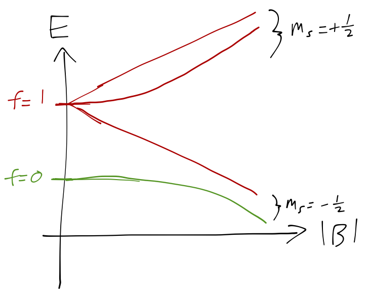
The full set of curves here relies on being careful about what happens at weak field values in order to match which state in the strong-field limit maps back to which of the \hat{\vec{F}}^2 eigenstates at zero magnetic field; see the Feynman lectures, chapter 12 if you’re interested in seeing all the details. (The weak-field calculation is similar to what we did for 2p hydrogen in Section 14.4.1 , or what we will do later with the Wigner-Eckart theorem for the Zeeman effect.) This is all sort of analogous to the Paschen-Back effect on the electron energy levels, where for a strong enough field we can “force” the energy eigenstates away from the total-spin \ket{f m_f} states and towards the product-basis \ket{m_s m_i} states.
22.7 Collected results for n=1 and n=2 hydrogen
Let’s combine everything that we’ve found so far and sketch a complete diagram of the energy eigenvalues for the first two hydrogen orbital levels. (I will include the n=2 hyperfine corrections in my sketch, although we won’t work them out explicitly here.) This diagram is just a sketch, and is certainly not to scale!
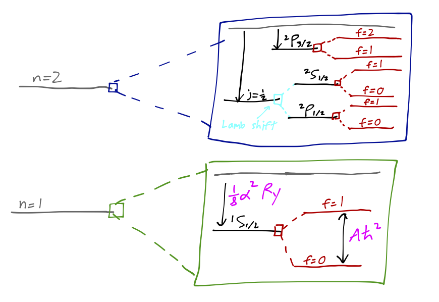
The value of the hyperfine splitting of 1s hydrogen is worth a closer look. If we calculate the energy difference between the f=1 and f=0 levels and convert to a light frequency by E = h \nu, we find that \nu = \frac{A\hbar}{2\pi} = 1420.406...\ \textrm{MHz} or in terms of a wavelength, \lambda = 21 cm. This radio-frequency light (also known as the “H-I spectral line”) is extremely important to astrophysicists, because interstellar space is full of dust which can block substantial amounts of visible light, but which is mostly transparent to radio frequencies. This transition giving rise to the 21 cm light, incidentally, can be thought of as a rather simple ``spin-flip” transition in which the spins of the electron and proton go from parallel to anti-parallel. This fact was famously memorialized on the golden plaque attached to the Pioneer and Voyager space probes with the following diagram:
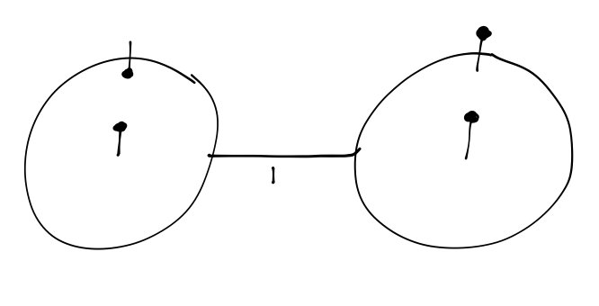
The other contents of the plaque use the 21cm line to provide units of time and length.