8 Wave mechanics and probability currents
Now we’re ready to make contact with wave mechanics; solution of the Schrödinger wave equation for the position-space energy eigenfunctions \psi(x). This is likely familiar from your undergrad quantum mechanics. I will show some elementary examples of solving problems and matching boundary conditions, but my main goal here will be linking these solutions to a broader discussion of probability currents, and physical interpretation of our solutions in terms of moving particles.
For all of its virtues, Sakurai is a bit light on examples, particularly in wave mechanics; I’ll be drawing heavily on other resources here, mainly the books by Merzbacher and Cohen-Tannoudji. I’ll try to show everything in a self-contained way in my own lecture notes, and some results are briefly collected in Appendix B of Sakurai (which I believe is expanded a bit in the newest edition.)
As a reminder, our starting point is the Hamiltonian for a particle of mass m in a one-dimensional potential V(x), which as an operator becomes \hat{H} = \frac{\hat{p}^2}{2m} + V(\hat{x}). Our primary goal in these examples will be solution of the energy eigenvalue equation, \hat{H} \ket{E} = E \ket{E}, or in the \ket{x} position basis, -\frac{\hbar^2}{2m} \frac{d^2 \psi_E}{dx^2} + V(x) \psi_E(x) = E \psi_E(x), which is the time-independent Schrödinger equation (or “TISE”). Solving for the energy eigenstates gives us everything we need to compute the dynamics, as we’ve seen previously. I will drop the E subscript and just write \psi(x) as is typical for solving these problems, but keep in mind that our solutions are always for a given energy E.
8.1 Example: potential step
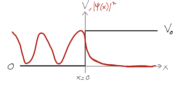
Our first example is the potential step, V(x) = \begin{cases} V_0, & x \geq 0 \\ 0, & x < 0. \end{cases}
In the region x < 0, the solutions to the TISE are simply plane waves, as we’ve seen before. To the right of the origin where V(x) = V_0 is a constant, the solutions are still plane waves: \psi(x) = A e^{ikx} + B e^{-ikx}, but now the wave number is computed from the energy difference, k = \sqrt{2m(E-V)}/\hbar. There are three interesting cases to consider here: E<0,\ E>V_0, and 0 \leq E \leq V_0. Let’s consider E<0 first; classically this solution corresponds to negative kinetic energy, and is forbidden. In quantum mechanics, it is still forbidden - the wavefunction can’t be normalized, as we have observed before, since k is imaginary everywhere (pure exponentials.)
8.1.1 Solution for 0 < E \leq V_0
For a classical particle in this case, we would find reflection by the barrier; when the particle reaches x=0, the sign of its momentum will be flipped, conserving total energy. Quantum mechanically, we know the form of the solution on either side of the barrier: \psi(x) = \begin{cases} A e^{ikx} + Be^{-ikx} & (x < 0), \\ C e^{-\kappa x} & (x > 0) \end{cases} where now we define the manifestly real quantities \hbar k = \sqrt{2mE}, \\ \hbar \kappa = \sqrt{2m(V-E)}. Notably, in the quantum system we find that our solution extends into the region x>0; the negative-exponential solution is normalizable, since it doesn’t extend to x = -\infty where it would blow up. The positive exponential e^{\kappa x} is still unphysical, so we discard it (its coefficient must be zero - see our previous discussion on quantum bound states, although this is not a bound state since the boundary is one-sided.)
We can determine the coefficients A,B,C from the boundary condition, which is that our wavefunction \psi(x) and its derivative should both be continuous across the jump in the potential. It’s easy to see why continuity is required, in fact for any potential function V(x) with a discontinuous jump at x_0. If we take the Schrödinger equation and integrate from x_0 - \epsilon to x_0 + \epsilon for some infinitesmal \epsilon, then we find \psi'(x_0 + \epsilon) - \psi'(x_0 - \epsilon) = \int_{x_0 - \epsilon}^{x_0 + \epsilon} dx \frac{2m}{\hbar^2} \left[ V(x) - E \right] \psi(x) Since \psi(x) itself can’t diverge (doing so would violate the probability interpretation), as long as V(x) is finite the integral will give a finite result that must vanish as \epsilon \rightarrow 0, and so the derivative \psi'(x) must be continuous across the potential jump. If the derivative is continuous, then so is \psi(x) itself.
In wave mechanics, if the potential V(x) has a sudden but finite change at point x_0, then the appropriate boundary conditions on the wavefunction solutions \psi_<(x) and \psi_>(x) defined for x < x_0 and x > x_0 are continuity of the wavefunction and its first derivative:
\psi_<(x_0) = \psi_>(x_0), \\ \psi_<'(x_0) = \psi_>'(x_0).
In the fine print above, we note that the potential change must be finite. If the potential barrier is infinite, then the conditions are different, as can be understood from our integral derivation above. In an extended region where the potential is infinite (like the infinite well), we simply have that \psi(x), \psi'(x), ... = 0 in that region.
The more interesting case is a delta-function boundary, for example V(x) = a \delta(x-x_0). We can go back to the derivation above to see how to deal with this: \psi'(x_0 + \epsilon) - \psi'(x_0 - \epsilon) = \int_{x_0-\epsilon}^{x_0+\epsilon} dx \frac{2m}{\hbar^2} \left[ a \delta(x-x_0) - E \right] \psi(x) \\ = \frac{2ma}{\hbar^2} \psi(x_0) so we find (a very specific) discontinuity in the derivative of the wavefunction. The wavefunction itself will be continuous across the delta function, since there’s only a finite jump in the derivative of \psi(x).
Since we’re talking about boundary conditions and derivatives, it’s natural to ask about the higher derivatives of the wavefunction \psi(x) - do those satisfy some sort of boundary condition as well? As with the lower-order boundary conditions, the answer can be found in the TISE. In this case, we don’t even need to integrate. Here it is again:
-\frac{\hbar^2}{2m} \frac{d^2 \psi_E}{dx^2} + V(x) \psi_E(x) = E \psi_E(x)
We can simply read off from the equation the fact that if V(x) is continuous, then so is \psi''(x). This extends to all higher derivatives: if V(x) is smooth (math terminology meaning “the function and all derivatives are continuous”), then so is \psi_E(x).
On the other hand, we see that even for the present example of the potential step, \psi_E(x) is definitely not smooth; there will be a step in \psi''_E(x) at x=0.
Now let’s go back to our piecewise solution with 0 < E \leq V_0 and apply the boundary conditions. Continuity of the wavefunction and its derivative at x=0 gives us two equations, A + B = C \\ ik(A-B) = -\kappa C. which we can solve for the ratios \frac{B}{A} = \frac{ik + \kappa}{ik - \kappa} \\ \frac{C}{A} = \frac{2ik}{ik - \kappa} = 1 + \frac{B}{A}. It’s convenient to notice that B/A is a pure phase; if we multiply by its complex conjugate, we find obviously that |B/A| = 1, so we can write it as \frac{B}{A} = e^{i\alpha} for some real number \alpha. Now let’s plug back in to our general solution. To the left of the barrier, we have \psi_<(x) = Ae^{ikx} + Be^{-ikx} \\ = A \left( e^{ikx} + e^{i\alpha} e^{-ikx} \right) \\ = Ae^{i\alpha/2} \left( e^{ikx - i\alpha/2} + e^{-ikx + i\alpha/2} \right) \\ = 2A e^{i\alpha/2} \cos\left( kx - \frac{\alpha}{2} \right). To the right: \psi_>(x) = Ce^{-\kappa x} \\ = A (1 + e^{i\alpha}) e^{-\kappa x} \\ = 2A e^{i\alpha / 2} \cos \left( \frac{\alpha}{2} \right) e^{-\kappa x}. So, the combined solution takes the form \psi(x) = \begin{cases} 2A e^{i\alpha / 2} \cos \left( kx - \frac{\alpha}{2} \right) & (x<0) \\ 2A e^{i\alpha / 2} \cos \frac{\alpha}{2} e^{-\kappa x} & (x>0). \end{cases} Notice that in this case, it didn’t matter what the energy E was; we could always find a solution which smoothly joined the exponential and plane-wave pieces of the wavefunction together. So the allowed energy E is continuous here.
How do we physically interpret this wavefunction? First, we should notice that unlike the classical case, the quantum particle has a non-zero probability |\psi(x)|^2 to be found in the classically forbidden region x>0; this probability is exponentially damped as x increases.
If we really want to expand the solution out in full for a specific energy, we need to solve for \alpha; it’s straightforward to write a formula for \tan \alpha in terms of E and V_0 using what we’ve defined above, but the result isn’t very enlightening, so I won’t bother to write it out.
8.1.2 Solution for E > V_0
Classically, a particle incident from the left with energy greater than V_0 will continue moving to the right, but its velocity will decrease when it encounters the potential step. In the quantum system, we now have oscillating solutions on both sides of the step: \psi(x) = \begin{cases} A e^{ikx} + Be^{-ikx}, & (x<0) \\ C e^{ik'x} + De^{-ik'x}, & (x>0) \end{cases} where k=\sqrt{2mE}/\hbar as before, and k'=\sqrt{2m(E-V_0)}/\hbar. Now we have something which is a bit puzzling at first glance: we still have only two boundary conditions, but now we have an extra unknown (complex) coefficient. How can we deal with this?
Physically, the extra missing boundary condition has to do with how we think about the boundary at x = \pm \infty. If we restore the time evolution, the two plane waves A and D represent incoming particles from infinity. So in an experimental situation, A and D are inputs to our solution, based on where our incoming particles are coming from (or if both directions are active, the relative intensity.)
In the simplest case with a straightforward interpretation as a single incoming particle, we should consider either A or D being non-zero. Let’s take D=0, so our incoming wave is A, from the left. Then we find for the boundary conditions at zero A + B = C \\ k(A-B) = k'C leading to the results \frac{B}{A} = \frac{k-k'}{k+k'} \\ \frac{C}{A} = \frac{2k}{k+k'}.
Now let’s think again about the physical interpretation of this solution. Just from the form of the solutions, we see that the classical behavior is reproduced here in the sense that k' < k, so the momentum is lower on the right side of the step (i.e. the particle indeed “slows down” after crossing the origin.)
Comparing to the solution with E \leq V_0, however, we see something very interesting and inherently quantum mechanical. In that previous case, the wavefunction only penetrates a finite difference into the barrier. Here, we see two waves appearing aside from our incoming wave A, one moving to the right (C) and one moving to the left (B) - so it seems that our particle is both moving past the barrier and bouncing off of it!
Let’s be more rigorous about these statements, by looking more carefully at the time dependence of probability in quantum mechanical systems.
8.2 Probability density and flux; the continuity equation
The idea of a probability current follows naturally from thinking about time-evolution of |\psi(x)|^2, which we know is a probability density. If we differentiate the probability density with respect to time, we find i\hbar \frac{\partial}{\partial t} (\psi^\star \psi) = i \hbar \frac{\partial \psi^\star}{\partial t} \psi + \psi^\star i\hbar \frac{\partial \psi}{\partial t} \\ = \psi^\star \left(-\frac{\hbar^2}{2m} \nabla^2 \psi + V \psi\right) - \left(-\frac{\hbar^2}{2m} \nabla^2 \psi^\star + V \psi^\star\right) \psi. where I’m working now in three-dimensional notation to derive the more general result, but you can read \nabla as d/dx for the one-dimensional case. The V \psi^\star \psi terms cancel out, and we can rewrite the other terms in a more symmetric way by moving one of the gradients outside, leading to \frac{\partial (\psi^\star \psi)}{\partial t} + \frac{\hbar}{2mi} \nabla \cdot \left[ \psi^\star \nabla \psi - (\nabla \psi^\star) \psi \right] = 0 \\ \Rightarrow \frac{\partial \rho}{\partial t} + \nabla \cdot \vec{j} = 0. This is exactly the form of a continuity equation, which you’ll recognize from e.g. classical electromagnetism; the rate of change of the local density is balanced by the divergence of the local current.
The flow of probability density for the wavefunction \psi(x) is encoded in the continuity equation \frac{\partial}{\partial t} (\psi^\star \psi) = -\nabla \cdot \vec{j}, where the probability current or probability flux \vec{j} is \vec{j} = \frac{\hbar}{2mi} \left[ \psi^\star \nabla \psi - (\nabla \psi^\star) \psi \right] = \frac{\hbar}{m} \textrm{Im} (\psi^\star \nabla \psi).
This is where the phase of the wavefunction, which cancels out in the local probability density, really has a physical effect. In fact, if we write explicitly \psi = \sqrt{\rho} e^{iS/\hbar} where both \rho and S are real (and the probability density \rho > 0), then the flux becomes \textrm{Im} \left(\psi^\star \nabla \psi\right) = \textrm{Im} \left( \sqrt{\rho} \nabla (\sqrt{\rho}) + \frac{i}{\hbar} \rho \nabla S \right) and so \vec{j} = \frac{\rho \nabla S}{m}. So the gradient of the phase of the wavefunction encodes the strength of the probability current.
Notice that this derivation depended on the fact that V(x) is real, i.e. that the Hamiltonian operator was Hermitian. The conservation of probability implied by the continuity equation is only valid if \hat{H} is Hermitian. This doesn’t mean that we should never consider a complex Hamiltonian; in fact, such an operator is useful for describing processes which are not conservative, e.g. decay or absorption of particles. We’ll see an explicit example of that a bit later.
8.2.1 Probability flux and the potential step
Back to our potential step example; what does the flow of probability look like in our solved example? First looking at 0 < E < V_0, we compute the product that determines \vec{j}: \psi^\star \frac{d\psi}{dx} = \begin{cases} 4|A|^2 k \cos \left(kx - \frac{\alpha}{2}\right) \sin \left(kx - \frac{\alpha}{2} \right) & (x<0), \\ -4|A|^2 \kappa \cos \frac{\alpha}{2} e^{-\kappa x} & (x>0). \end{cases} This has zero imaginary part in both regions, so we conclude that \vec{j} = 0 everywhere; there is no net flow of probability in this solution.
To understand this more deeply, notice that because (writing the left-side solution in the original form Ae^{ikx} + Be^{-ikx}) the ratio B/A = e^{i\alpha} is a pure phase, we have |A|^2 = |B|^2. We can think of A and B as probability amplitudes associated with a right-moving and left-moving plane wave, respectively; the waves having equal (squared) amplitudes therefore corresponds to total reflection. Indeed, if we construct a wave-packet solution out of solutions with 0 < E < V_0 and send it towards the barrier, it will end up propagating back to the left with the same amplitude as the incident packet, despite the fact that it may temporarily penetrate the barrier at x=0.
I’ll note in passing that if you did the exercise with an incoming wave packet, you would not find \vec{j} = 0 everywhere, since the probability density will be evolving in time as the packet moves. The solutions \psi(x) we’re looking at are energy eigenstates; since such a state only evolves in time by picking up a phase factor e^{iEt/\hbar}, the product \psi^\star \psi will be constant; this implies that we must always find a constant probability current for an energy eigenstate, so that \partial \rho / \partial t = -\nabla \cdot \vec{j} = 0.
Now we return to the other case with E > V_0. Here the ratios B/A and C/A are no longer pure phases, and correspondingly if we calculate the probability flux now, we no longer find zero: j = \begin{cases} \frac{\hbar k}{m} (|A|^2 - |B|^2), & (x<0) \\ \frac{\hbar k'}{m} |C|^2, & (x>0). \end{cases}
Now, we’re still studying an energy eigenstate, which means that the gradient of the probability current is still zero everywhere, including at x=0; this means that the two constants above must be equal, leading to the requirement that \frac{|B|^2}{|A|^2} + \frac{k'}{k} \frac{|C|^2}{|A|^2} = 1. (This is not a new constraint: if we plug in B/A and C/A from above, it just reduces to 1=1. This has to be true, since the continuity equation is not a new constraint either, we derived it from the TISE! But continuity gives another way to derive the relation between these ratios, which can be useful when it’s harder to solve directly.)
The ratios B/A and C/A tell us the relative amplitude of the reflected and transmitted waves with respect to the incident wave, respectively. They also directly determine the size of the probability current \vec{j}; as B/A decreases, the value of the current increases. All of this motivates defining, in analogy to optics, the reflection and transmission coefficients: R = \frac{|B|^2}{|A|^2} = \frac{(k-k')^2}{(k+k')^2} \\ T = \frac{k'}{k} \frac{|C|^2}{|A|^2} = \frac{4kk'}{(k+k')^2}. Notice that the continuity equation tells us that R+T=1; this is the condition for conservation of probability.
This is now obviously non-classical behavior; even though we are treating a single particle moving in a simple potential, it seems to “break apart” into reflected and transmitted pieces at the barrier. Reconciling this result with the fact that we see indivisible, identical particles like electrons strongly motivates particle-wave duality and the probability interpretation of the wave!
8.3 Example: rectangular barrier
Now we can move on to a slightly more complicated system, the rectangular barrier potential: V(x) = \begin{cases} V_0, & |x| < a, \\ 0, & |x| > a. \end{cases} The most interesting case this time is E < V_0.
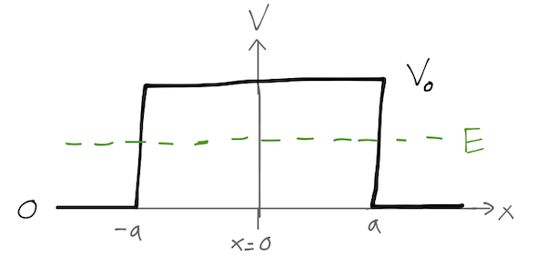
Once again the potential is piecewise constant, so we can start by writing down the solution to the Schrödinger equation, now in three parts: \psi(x) = \begin{cases} A e^{ikx} + Be^{-ikx}, & (x < -a); \\ C e^{-\kappa x} + De^{\kappa x}, & (-a < x < a); \\ F e^{ikx} + Ge^{-ikx}, & (x > a). \end{cases} with k and \kappa defined as above. Matching boundary conditions at the left boundary first, we have the pair of equations Ae^{-ika} + Be^{ika} = Ce^{\kappa a} + De^{-\kappa a} \\ Ae^{-ika} - Be^{ika} = \frac{i\kappa}{k} (Ce^{\kappa a} - De^{-\kappa a}). This is best re-expressed as a matrix equation: \left( \begin{array}{c} A \\ B \end{array} \right) = \left( \begin{array}{cc} M_{11} & M_{12} \\ M_{21} & M_{22} \end{array} \right) \left( \begin{array}{c} F \\ G \end{array} \right). where I am not explicitly writing out the components of the matrix M; they are fully determined by k and \kappa, but that isn’t what I want to focus on. Rewriting like this eliminates C and D, which for most realistic experiments is just what we want: in the context of scattering, for example, we’re more interested in how an incoming particle is related to an outgoing one than what happens in the middle of the potential barrier.
In fact, in the context of experiment it’s much more natural to ask about how the “output” waves are related to the “input” waves. Identifying the incoming waves as right-mover A and left-mover G, we can relate them to the outgoing B and F by reorganizing to get a different matrix: \left( \begin{array}{c} F \\ B \end{array} \right) = \left( \begin{array}{cc} S_{11} & S_{12} \\ S_{21} & S_{22} \end{array} \right) \left( \begin{array}{c} A \\ G \end{array} \right). (the ordering on the left is chosen because F is the transmitted wave from incoming wave A.) The M matrix is easier to work with in one-dimensional problems, but this S-matrix can be generalized to three dimensions easily, and gives us the best way to state certain symmetry properties. In particular, the properties of the S-matrix are intimately linked to the probability currents we introduced above.
For a steady-state solution (i.e. the wavefunction of an energy eigenstate), there can be no net flow of probability, which means that the divergence \nabla \cdot \vec{j} = 0. For our potential-barrier wavefunction, we have to the left of the barrier \vec{j} = \frac{\hbar}{m} \textrm{Im} \left(\psi^\star \frac{\partial \psi}{\partial x}\right) \\ = \frac{\hbar}{m} \textrm{Im} \left[ \left( A^\star e^{-ikx} + B^\star e^{ikx} \right) \left(ikA e^{ikx} - ikB e^{-ikx} \right)\right] \\ = \frac{\hbar}{m} \textrm{Im} \left[ ik (|A|^2 - |B|^2) - ikA^\star B e^{-2ikx} + ikB^\star A e^{2ikx} \right] \\ = \frac{\hbar k}{m} (|A|^2 - |B|^2) since \textrm{Im}(i(z - z^\star)) = 0. Similarly, on the right side the current is equal to \vec{j} = \hbar k/m (|F|^2 - |G|^2)). The condition inside the barrier isn’t so important, if we’re interested in the scattering of incoming waves. In terms of the external solutions, we find that conservation of probability implies |A|^2 - |B|^2 = |F|^2 - |G|^2 \\ \Rightarrow |B|^2 + |F|^2 = |A|^2 + |G|^2. This is what you would have expected from conservation of probability; the total incoming probability current equals the total outgoing current. We can rewrite this equation in matrix notation, \left( A^\star\ \ G^\star\right) \left(\begin{array}{c} A \\ G \end{array}\right) = \left( F^\star\ \ B^\star\right) \left(\begin{array}{c} F \\ B \end{array}\right) = \left( A^\star\ \ G^\star\right) (S^\dagger S) \left(\begin{array}{c} A \\ G \end{array}\right) . So conservation of probability implies that the S-matrix is unitary. This simple observation remains true even in higher dimensions and more complicated systems, and regardless of the form of the potential barrier itself. We’ll return to studying the S-matrix as part of a more formal discussion of scattering theory much later.
Let’s go back to finish our example for the potential step, going to the case where we have an incident particle from the left so that G=0. I’ll skip the algebra, but it’s not too hard to show that the ratio of the transmitted to incident amplitude is \frac{F}{A} = \frac{e^{-2ika}}{\cosh 2\kappa a + i(\epsilon/2) \sinh 2\kappa a} where again k = \sqrt{2mE}/\hbar, \kappa = \sqrt{2m(V_0 - E)}/\hbar, and I’ve defined \epsilon = \frac{\kappa}{k} - \frac{k}{\kappa} = \frac{\sqrt{V_0-E}}{\sqrt{E}} - \frac{\sqrt{E}}{\sqrt{V_0-E}} = \frac{1-2E/V_0}{\sqrt{E/V_0 (1-E/V_0)}}. As we adjust the ratio E/V_0, this function diverges to +\infty at small E and -\infty for E approaching V_0, with a zero at E = 2V_0. Squaring the amplitude ratio gives us the transmission coefficient: T = \frac{|F|^2}{|A|^2} = \frac{1}{\cosh^2 2\kappa a + \frac{1}{4} \epsilon^2 \sinh^2 2\kappa a} This is, in general, a fairly complicated function depending on two parameters, the relative barrier height V_0/E and the relative barrier width \kappa a. There are some interesting limits to consider. First, if the barrier is very wide so that \kappa a \gg 1, then \cosh 2\kappa a \approx \sinh 2 \kappa a \approx e^{2\kappa a}/2 which leads to the result T \approx 16 e^{-4 \kappa a} \left( \frac{k \kappa}{k^2 + \kappa^2} \right)^2 = 16 e^{-4\kappa a} \left( \frac{V_0/E - 1}{(V_0/E-1)^2 + 1} \right)^2
(Keep in mind that we approximated \kappa a \gg 1, which means that this formula is definitely invalid for E \approx V_0, which corresponds to \kappa \rightarrow 0.)
Notice that the tunneling coefficient is exponentially sensitive to the width of the barrier 2a! This simple model illustrates the basic idea behind scanning tunneling microscopy; here the gap of air between a very small probe and a surface of some material serves as the potential barrier. Electrons tunneling from the surface to the probe give rise to a small tunneling current; by moving the microscope probe across the surface and adjusting its height to keep the measured current constant, it is possible to create a contour map of the surface.
On the other hand, if the barrier is very high, then V_0 \gg E which implies that \kappa \gg k; we also take it to be narrow, so \kappa a \ll 1. From the definition above we see that \epsilon \approx \kappa/k, and so T \approx \frac{k^2}{k^2 + \kappa^4 a^2} = \frac{1}{1 + \frac{2mV_0}{\hbar^2} a^2 (V_0/E)}. The transmission rate now goes to 1 in the limit of an infinitely narrow barrier, but goes to 0 as the barrier height increases. If we take a combined limit which preserves the area under the barrier, i.e. g = \lim_{a \rightarrow 0, V_0 \rightarrow \infty} V_0 (2a) then the transmission rate is determined by g, T = \frac{E}{E + \frac{mg^2}{2\hbar^2}}. This is, in fact, exactly the result we would obtain if we started with a delta-function potential, V(x) = g \delta(x).
What about the case where the energy is above the potential barrier, E > V_0? We don’t actually have to go back and solve the Schrödinger equation from scratch. We have been dealing with two sorts of solutions to the Schrödinger equation in a constant potential, either plane waves e^{\pm ikx} or exponential decay and growth, e^{\pm \kappa x}. But the latter is really just a plane-wave solution where the wave number k = \sqrt{2m(E-V_0)} / \hbar has become imaginary. Similarly, we can consider a plane-wave solution to be an exponential with imaginary \kappa. So if we go back to our solution and simply replace \kappa \rightarrow -ik', where k' = \sqrt{2m(E-V_0)}/\hbar, then we have T = \frac{1}{\cos^2 2k'a - \epsilon^2/4 \sin^2 2k'a} where I’ve used the identities \cosh(-ix) = \cos(x) and \sinh(-ix) = -i \sin(x). This looks like it might blow up at certain values of E/V_0, but of course \epsilon is a function of E/V_0 too. If we plug in \epsilon as a function of E/V_0 and manipulate a bit, we can find the expression T = \left[ 1 + \frac{\sin^2 (2k' a)}{4E/V_0 (E/V_0 - 1)}\right]^{-1}. This transmission coefficient is now well-behaved, since the second term is always positive. Moreover, we can notice from this expression that whenever 2k'a = n\pi, we actually have T=1 (and therefore R=0.) These points where the transmission is maximum are known as transmission resonances.
![]()
Here I show the two solutions for E/V_0 < 1 and E/V_0 > 1 joined together for some arbitrary numerical values; notice the transmission resonances at positive E/V_0.
8.4 Parity
Before we continue, let’s pause briefly to consider our first example of a symmetry, which will help to simplify the next calculation we do. The simple yet powerful symmetry that we will study is parity, also known as mirror reflection. Parity flips our coordinate system backwards: in one dimension, it takes x \rightarrow -x and p \rightarrow -p. (It will, in general, reverse the sign of any vector quantity - we just don’t usually label vectors explicitly in one dimension, so we need to be a little careful! Even though we’re in 1-d at the moment, I’m going to write x as \vec{x} for a bit - this also makes it easy to generalize what I will say here to higher dimensions.)
In quantum mechanics, we construct a parity operator \hat{P} that accomplishes this transformation. We will start in the operator picture and define it in terms of how it acts on our operators: for example, for the position operator it must act as \hat{P}{}^\dagger \hat{\vec{x}} \hat{P} = -\hat{\vec{x}} (and the same for \hat{\vec{p}} or any other vector operator, as noted.)
The parity operator has to be unitary: we can see that by applying it to the dot product of two vectors, which should itself be invariant under parity: \hat{P}{}^\dagger \hat{\vec{x}} \hat{P} \cdot \hat{P}{}^\dagger \hat{\vec{x}} \hat{P} = \hat{\vec{x}} \cdot \hat{\vec{x}} = \hat{P}{}^\dagger (\hat{\vec{x}} \cdot \hat{\vec{x}}) \hat{P} so \hat{P}{}^\dagger = \hat{P}{}^{-1}, i.e. \hat{P} is unitary (as it should be to describe a symmetry.)
Going back towards wave mechanics, what does parity do to our wavefunctions? This is more useful to think about in the passive transformation picture where our states change instead of our operators. We can relate the two by writing \bra{\vec{x}'} \hat{\vec{x}} \ket{\vec{x}} \rightarrow \bra{\vec{x}'} \hat{P}^\dagger \hat{\vec{x}} \hat{P} \ket{\vec{x}} \\ = \bra{\vec{x}'} -\hat{\vec{x}} \ket{\vec{x}} = - \vec{x} \delta(\vec{x} - \vec{x}') = -\vec{x}' \delta(\vec{x} - \vec{x}') so we see that (as we might have guessed) parity is flipping the sign of our position eigenvalues, \hat{P} \ket{\vec{x}} = \ket{-\vec{x}}.
This means that the wavefunction transforms as \psi(\vec{x}) = \left\langle \vec{x} | \psi \right\rangle \rightarrow \bra{\vec{x}} \hat{P} \ket{\psi} = \left\langle -\vec{x} | \psi \right\rangle = \psi(-\vec{x}). In fact, from the states it’s easy to see that \hat{P} is more than just unitary: if we apply parity twice, then \hat{P}^2 \ket{\vec{x}} = \hat{P} \ket{-\vec{x}} = \ket{+\vec{x}} so we also have \hat{P}{}^2 = \hat{1}; in other words, \hat{P} is its own inverse. (If you are familiar with group theory, this last property indicates that the symmetry group associated with parity is \mathbb{Z}_2. More on symmetry and groups later on.)
What do the parity eigenstates look like? If \ket{P} is a parity eigenstate, then we have \hat{P} \ket{P} = P \ket{P}. But \hat{P}{}^2 \ket{P} = P \hat{P} \ket{P} = P^2 \ket{P} = \ket{P} so P^2 = 1, i.e. the eigenvalues of parity are always P = \pm 1.
The action of parity on the Hamiltonian is particularly interesting. If we find parity is a dynamical symmetry, i.e. [\hat{P}, \hat{H}] = 0, then we will be able to construct simultaneous eigenkets of \hat{P} and \hat{H} (which will then stay as parity eigenstates for all time, since time evolution will commute with parity - hence, “dynamical symmetry”!). The momentum part of the Hamiltonian is proportional to \vec{p} \cdot \vec{p}, and as we saw above, the dot product of a vector with itself is parity invariant, so \hat{H} is invariant if the potential is invariant, V(\vec{x}) = V(-\vec{x}). For a potential satisfying this condition (like our square well), any eigenket of \hat{H} is also an eigenket of \hat{P}.
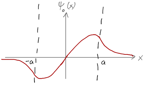
Any energy eigenfunction \psi(x) can therefore be identified as either a positive-parity or even state, with P=1, or a negative-parity or odd state with P=-1. We can see what this implies for the spatial wavefunctions: if \ket{\psi} is an energy/parity eigenstate, then \left\langle x | \psi \right\rangle = \bra{x} \hat{P} \hat{P} \ket{\psi} = P \left\langle -x | \psi \right\rangle. So in other words, the even-parity wavefunctions satisfy \psi_e(\vec{x}) = \psi_e(-\vec{x}) and the odd-parity ones satisfy \psi_o(\vec{x}) = - \psi_o(-\vec{x}).
8.5 Example: the square well
Now that we have parity as a tool, let’s attack another simple wave mechanics example by taking our potential barrier and flipping it upside down, i.e. taking V_0 to -V_0; this gives us the square well potential: V(x) = \begin{cases} -V_0, & |x| < a \\ 0, & |x| > a. \end{cases}
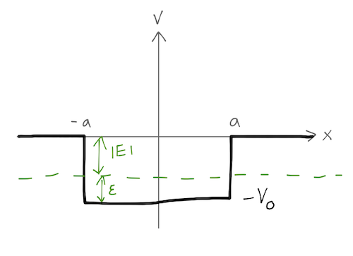
We’ll begin with the case where -V_0 < E < 0, looking for bound states. If we let \epsilon = E + V_0 = V_0 - |E| be the distance between the energy and the bottom of the well, then the wave number inside the well is the usual k = \sqrt{2m\epsilon} / \hbar. The exponential decay constant outside the well is \kappa = \sqrt{2m|E|} / \hbar. The general solution looks like \psi(x) = \begin{cases} B_+ e^{+\kappa x}, & (x < -a); \\ A_+ e^{ikx} + A_- e^{-ikx}, & (-a < x < a); \\ B_- e^{-\kappa x}, & (x > a). \end{cases}
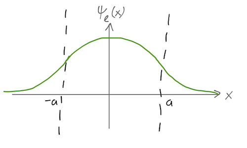
However, instead of solving this directly, we first notice that because the potential is symmetric in x, parity commutes with our Hamiltonian. Thus, we know that we can split the solutions into those with even parity, \psi_e(x) = \begin{cases} A \cos kx, & |x| < a; \\ B e^{-\kappa |x|}, & |x| > a. \end{cases}
and those with odd parity, \psi_o(x) = \begin{cases} A' \sin kx, & |x| < a; \\ B' e^{-\kappa x}, & x > a; \\ -B' e^{\kappa x}, & x < a. \end{cases}
So we’ve immediately reduced our unknown coefficients from 4 down to 2 for each subset of solutions. We’ve also reduced the number of constraints from continuity to 2, since continuity of \psi(x) and its derivative at x = +a now also guarantees it at the reflected boundary x = -a. There is one more constraint, overall normalization of the wavefunction; only certain values of the energy E will allow us to satisfy all constraints, as expected for bound states.
Let’s start with the even-parity solution. Applying the boundary condition at x=a (the other boundary is redundant thanks to parity!) to this state gives A \cos ka = B e^{-\kappa a} \\ -Ak \sin ka = -B\kappa e^{-\kappa a} which can be combined to obtain a condition on the wave numbers and thus the allowed energy E: ka \tan ka = \kappa a. Similarly, for the odd-parity states we find ka \cot ka = -\kappa a. Now let’s define for convenience the parameters \xi \equiv ka and \eta \equiv \kappa a. From the definitions of k and \kappa, we see that \xi^2 + \eta^2 = \frac{2ma^2}{\hbar^2} (E + V_0 - E) = \frac{2ma^2}{\hbar^2} V_0, while from above we have (for even parity) \xi \tan \xi = \eta. This is a transcendental equation, so we can’t find a closed-form solution. However, we can solve this pair of equations graphically. If we plot \eta vs. \xi, then the first equation above defined a circle with radius \sqrt{2mV_0} a/\hbar; solutions occur wherever this circle intersects the function \xi \tan \xi.
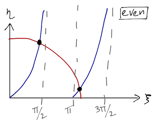
These are solutions for the bound-state energy E, which determines the values of k and \kappa. Notice that even as the radius of the circle vanishes, we will always find at least one even-parity bound state. As the radius rises (the well becomes deeper or wider), the number of solutions increases. If we take V_0 \rightarrow \infty then we find an infinite number of bound-state solutions, corresponding to the (even-parity) standard results for the infinite square well.
What about the odd-parity solutions? We have the same equation for the circular curves, but now the boundary conditions instead yield the relation \xi \cot \xi = -\eta.
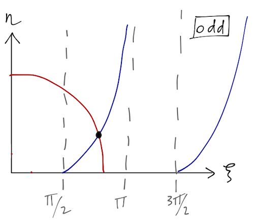
Now we see that there will be no solutions if \sqrt{2mV_0} a/\hbar < \pi/2; if the potential well is too shallow, there are no odd-parity bound states.
For completeness, I’ll note that we can also study scattering from the square well, i.e. solutions with E>0. We will find similar results to what we had for the barrier before: I won’t go through the details, but in particular we find for the transmission coefficient T = \left(1 + \frac{\sin^2(2k'a)}{4E/V_0(E/V_0+1)} \right)^{-1}. so we once again have resonance at precisely the values 2k'a = n\pi. (However, note that the definition of k' has changed: for the potential barrier we had k' = \sqrt{2m(E-V_0)}/\hbar, while for the well it is k' = \sqrt{2m(E+V_0)}/\hbar.)
We can think about this more physically to understand the source of the resonant behavior. Remember that at any barrier, a quantum-mechanical particle will undergo both transmission and reflection (this is possible because the wavefunction allows a single particle to be non-localized in a sensible way.) Although we’ve focused on the final transmission amplitude, there is generically transmission and reflection at both edges of the barrier. In particular, some part of the incident plane wave A will be reflected internally some number of times before finally being transmitted into outgoing wave F. The condition 2k'a = n\pi can be rewritten as 4a = n (2\pi/k'), in other words, transmission resonance occurs when the distance 4a traveled by an internally reflected wave is equal to an integer multiple of the de Broglie wavelength (2\pi/k'), resulting in constructive interference.