13 Spin in quantum mechanics
As part of our larger discussion on angular momentum operators, let’s turn now to spin. Spin is distinct from orbital angular momentum in that we think of it as an intrinsic property of a particle, one that doesn’t require considering motion in space at all. (Very roughly, you can think of this as the particle itself “spinning” in place, although this interpretation will break if you try to compare it to a literally spinning ball of mass.)
One of the facts we noticed about orbital angular momentum was that the quantum number \ell of the \hat{L}^2 operator could only take on integer values. This also maps nicely on to how we think about the dimension of the Hilbert space of angular momentum eigenstates. Recall that the eigenvalue equations defining the \ket{\ell, m} states are \hat{L}^2 \ket{\ell, m} = \hbar^2 \ell(\ell+1) \ket{\ell, m} \\ \hat{L}_z \ket{\ell, m} = \hbar m \ket{\ell, m} and the two quantum numbers (often called “orbital” and “magnetic” quantum numbers e.g. for hydrogen) are related by the condition |m| \leq \ell. This means that if we fix the orbital quantum number, the dimension of the state (sub)space is d = 2\ell + 1.
This is, of course, familiar from classical mechanics. The \ell = 0 representation is a one-dimensional Hilbert space that doesn’t transform under rotations at all, corresponding to a scalar quantity like energy. If we have \ell = 1, then that is the next “smallest” object that transforms under rotation - a vector, with three components since we have three spatial dimensions. In quantum mechanics, the rotational components will form a three-dimensional Hilbert space consisting of \ket{1,0} and \ket{1,\pm 1}.
However, while only integer \ell makes sense for e.g. spherical harmonics, the algebra that we worked out for angular momentum operators is actually perfectly fine with half-integer eigenvalues as well. The smallest possibility is 1/2, which would correspond to a 2-component object that transforms non-trivially under rotation - something which is like a vector, but somehow smaller.
Of course, you know what this is already - it’s exactly the familiar spin-1/2 system that we’ve seen since lecture 1 in the Stern-Gerlach experiments. But take a moment to appreciate how weird this is classically; there is some object with less than three components which nevertheless transforms non-trivially under rotation!
13.1 Complete sets of commuting observables
This is a good point to more rigorously introduce the idea of a complete set of commuting observables (or CSCO.) As we have seen, the importance of finding a set of commuting observables, i.e. \hat{A}, \hat{B}, \hat{C}, ... such that [\hat{A}, \hat{B}] = [\hat{A}, \hat{C}] = [\hat{B}, \hat{C}] = 0, is that we can label eigenstates simultaneously with each of the eigenvalues \ket{a, b, c...}. A complete set of commuting observables occurs when we can uniquely label a complete basis of our Hilbert space with the eigenvalues in our set. In other words, using the eigenkets of our CSCO operators, we can uniquely specify any state at all in our Hilbert space as a list of eigenvalues (known in this context as the quantum numbers of a given eigenstate.)
Another way to state the significance of this last point is that if we measure every observable in our CSCO, we expect the system to collapse to a single, unique state which is a simultaneous eigenvector of all of the observables \ket{a,b,c...}. Thus, the CSCO represents the maximum set of things we can know simultaneously about our system. The ideal situation occurs when the Hamiltonian itself is part of our CSCO, since this makes the time evolution especially simple: any state in the CSCO just picks up a phase according to its energy.
It’s important to note that the choice of a CSCO is, in general, not unique. As a trivial example, for the simple two-state system we can use \hat{S}_x to label eigenstates just as well as \hat{S}_z. Moreover, we saw that we can construct the operator \hat{\vec{S}}^2 even in the two-state system, so \{\hat{\vec{S}}{}^2, \hat{S_z}\} could be a CSCO. However, we don’t gain any new information from \hat{\vec{S}}{}^2 in this case, since it is proportional to the identity. An even more pathological example comes from the simple harmonic oscillator, where we can construct the projection operators P_n = \ket{n}\bra{n}. These give an infinite CSCO; we can label all of the energy eigenstates uniquely as a binary string \ket{00100...}. This is obviously not efficient, but it does meet the mathematical definition of a CSCO. So there is no algorithm for determining a unique, best CSCO for a given problem; in practice, we look for the smallest CSCO we can find, and commuting with the Hamiltonian is a plus.
How do we know when we do not have a CSCO? The main requirement for such a set is that measuring all of the operators in it will result in a unique state, which means that there must be no degeneracy in the eigenvalues when we measure everything. Of course, an individual operator can still have degeneracy, as long as some other operator breaks the degeneracy, e.g. our set of unique eigenkets may contain the states \ket{a,b,c_1} and \ket{a,b,c_2}, where c_1 \neq c_2. If we find two states with degenerate eigenvalues for every operator in our set, then we don’t have a CSCO, and must find some new operator to add.
Now you should ask the question: how do we decide whether there is an unbroken degeneracy? A good, prototypical example is given by the hydrogen atom, which is usually first studied based on a CSCO consisting of \{\hat{H}_{\rm Coulomb}, \hat{L}^2, \hat{L}_z\} so that the basis states can be labelled with \ket{n,l,m}, just as we saw before with the isotropic harmonic oscillator. Of course, many of these energy levels are degenerate due to rotational invariance and accidental symmetry; if we only looked at the emission spectrum of hydrogen at a high level, we would only see the n quantum number. We have to probe with electric and magnetic fields that break the rotational invariance to see energy levels that depend on all three quantum numbers n,l,m, breaking the degeneracy.
But if we take our hydrogen atoms and put them in a magnetic field, we observe that the \ket{n,l,m} labels are not enough; there is an additional splitting of spectral lines, indicating there are more energy levels than our current basis describes, and requiring us to add a fourth quantum number m_s, corresponding to the spin \hat{S}_z of the orbital electron! But if we don’t apply a magnetic field to probe the system, it is impossible to tell that we’re missing anything from the \ket{n,l,m} basis and our original CSCO. In other words, whether we have found a CSCO is in fact an experimental question! If we perform different experiments on a system, measure different observables, then we can try to see if we’re missing any information, i.e. if a state we previously thought was a completely determined eigenstate splits into multiple possible outcomes.
13.2 Spin-1/2 revisited
Let’s see a little more about the spin-1/2 system with our new knowledge of how rotations work in quantum mechanics. What do finite rotations in a system with dimension-two angular momentum operators look like? If we fix our attention on the z axis, then the states rotate as \ket{\psi}_R = \exp \left( \frac{-i \hat{S}_z \phi}{\hbar} \right) \ket{\psi}. To check that this is really a rotation operator, we can look at its effect on the expectation value \left\langle \hat{S}_x \right\rangle: \left\langle \hat{S}_x \right\rangle \rightarrow \bra{\psi}_R \hat{S}_x \ket{\psi}_R = \bra{\psi} \exp \left( \frac{i \hat{S}_z \phi}{\hbar}\right) \hat{S}_x \exp \left( \frac{-i \hat{S}_z \phi}{\hbar} \right) \ket{\psi}, so we need to compute the commutator of \hat{S}_x with the rotation operator, \hat{U}_z. This is easy to do by expanding \hat{S}_x out as an outer product in the \hat{S}_z eigenbasis: \hat{S}_x = \frac{\hbar}{2} \left[ \ket{\uparrow} \bra{\downarrow} + \ket{\downarrow}\bra{\uparrow} \right] \\ \Rightarrow \hat{U}_z{}^\dagger \hat{S}_x \hat{U}_z = \frac{\hbar}{2} \left[ e^{i\phi/2} \ket{\uparrow} \bra{\downarrow} e^{i\phi/2} + e^{-i\phi/2} \ket{\downarrow} \bra{\uparrow} e^{-i\phi /2} \right] \\ = \frac{\hbar}{2} \left[ (\ket{\uparrow} \bra{\downarrow} + \ket{\downarrow} \bra{\uparrow}) \cos \phi + i (\ket{\uparrow}\bra{\downarrow} - \ket{\downarrow} \bra{\uparrow}) \sin \phi\right] \\ = \hat{S}_x \cos \phi - \hat{S}_y \sin \phi, exactly as we would expect for a rotation by \phi about the z-axis. This derivation required us to draw heavily on our existing knowledge of the two-state system, so you might worry about whether the same relation is true in general. In fact, it’s possible to derive the same result for any N using just the commutation relations and the Baker-Hausdorff formula; the details are in Sakurai if you’re curious.
Repeating this operation for the other expectation values finds similar results; in fact, the expectation value of the spin rotates just like an ordinary classical vector, \left\langle \hat{S}_k \right\rangle \rightarrow \sum_\ell R_{k\ell} \left\langle \hat{S}_\ell \right\rangle. Once again, this is easily derived for angular momentum operators with any dimensionality using the commutation relations, so \left\langle \hat{J}_k \right\rangle \rightarrow \sum_\ell R_{k\ell} \left\langle \hat{J}_\ell \right\rangle.
This is all very straightforward so far, but here comes the twist. What does the rotation operator (about z again) do to an arbitrary ket? Since we’re in a two-state system, it’s easy to expand in eigenstates of \hat{S}_z: \exp \left( \frac{-i \hat{S}_z \phi}{\hbar} \right) \ket{\psi} = e^{-i\phi /2} \ket{\uparrow}\left\langle \uparrow | \psi \right\rangle + e^{i\phi/2} \ket{\downarrow} \left\langle \downarrow | \psi \right\rangle. The factor of 1/2 in the rotation should worry you. In fact, it’s easy to see that a rotation by \phi = 2\pi, which we would normally expect to have no effect at all, changes the sign of the state: \ket{\psi}_{R(2\pi)} = -\ket{\psi}. At least for the state ket itself, our system now appears to be 4\pi periodic. This didn’t appear in the expectation values above, since the sign appears twice. Does this sign have any observable consequences? Obviously it didn’t affect the expectation values above, since the minus sign (also known as a \pi phase shift) just cancels out. The only way we will see an effect is to rotate part of our system, and compare it to an unrotated state.
13.2.1 Spin and representations of rotation
If you think back to our discussion of symmetry and rerpesentations, previously I told you that the rotation group SO(3) only has odd-dimensional representations. But we’re now working with rotations in a two-dimensional Hilbert space, so what gives?
In fact, the rotation matrices with half-integer angular momentum are not representations of SO(3)! To preserve the structure of the rotation group, a rotation by 2\pi has to be equal to the identity, but we’ve just seen that isn’t the case for spin-1/2; we get minus the identity. In terms of representations, we can phrase this as: the product of two rotations by \pi should give us back the identity, but we have \rho_2(\pi) \rho_2(\pi) \neq \rho_2(2\pi) = 1.
The trick is that half-integer angular momentum can be thought of as representations of rotation, if we relax our idea of a representation to something called a projective representation. A projective representation only preserves the group products up to a phase: in general, \rho(g_1) \rho(g_2) = e^{i\phi(g_1, g_2)} \rho(g_1 \cdot g_2).
You can see that this is true for our rotation above: the extra minus sign that appears with a 2\pi rotation is just a phase of \pi. It is generally true that all of the half-integer angular momentum representations are projective representations of SO(3).
The only reason that a projective representation is a reasonable thing to work with is because we’re doing quantum mechanics; picking up extra phases under symmetry operations is okay, because overall phases don’t change the physics! This is, basically, the reason why half-integer angular momentum is a uniquely quantum-mechanical phenomenon.
13.2.2 Spin-1/2 and measuring the phase shift
Of course, the spin of an electron isn’t an ordinary angular momentum; there’s no sense in which you can think of the electron as a spinning ball of charge with some finite extent. (High-energy scattering of electrons has confirmed that they have no “size” down to sub-femtometer distances.) The main way in which the spin of the electron manifests itself is through the magnetic moment, which in an external magnetic field gives the Hamiltonian term \hat{H} = \hat{\vec{\mu}} \cdot \hat{\vec{B}} = - \frac{e}{m_e c} \hat{\vec{S}} \cdot \hat{\vec{B}}.
If we choose, say, an electric field in the z-direction, then (as we have derived before) the result is a precession of the spin; the expectation values of the various components rotate as \left\langle \hat{S}_x \right\rangle \rightarrow \left\langle \hat{S}_x \right\rangle \cos \omega t - \left\langle \hat{S}_y \right\rangle \sin \omega t \\ \left\langle \hat{S}_y \right\rangle \rightarrow \left\langle \hat{S}_y \right\rangle \cos \omega t + \left\langle \hat{S}_x \right\rangle \sin \omega t \\ \left\langle \hat{S}_z \right\rangle \rightarrow \left\langle \hat{S}_z \right\rangle, where \omega = \frac{|e|B}{m_e c}. So application of a uniform magnetic field gives us a way to rotate the (average) electron spin orientation, as a function of time. This can be thought of, exactly as we derived above, a rotation of the state vector through angle \phi = \omega t. In fact, the state vector itself as a function of time is \ket{\psi(t)} = e^{-i\omega t/2} \ket{\uparrow} \left\langle \uparrow | \psi \right\rangle + e^{i\omega t/2} \ket{\downarrow} \left\langle \downarrow | \psi \right\rangle. Once again, the rotation has to go twice as far to return the original state vector, \tau_S = 4\pi/\omega, compared to the period of the observable spin precession \tau_P = 2\pi / \omega. We can now construct an experiment to see the effects of rotation, and we’ll turn to a simple two-slit interference setup (which we haven’t treated in detail in this course yet, but you should know enough about it from your previous quantum courses to follow:)
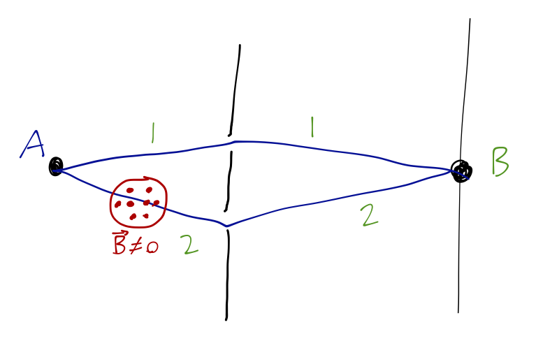
Nominally we use neutrons for this experiment, instead of electrons; neutrons also have spin-1/2 and a non-zero magnetic moment, but they don’t have any charge we don’t have to worry about the magnetic field significantly bending their trajectory. Denoting the amplitudes for traveling from A to B on the top and bottom paths as A_1 and A_2 respectively, we see that the effect of the magnetic field on the lower path will be A_2 = A_2(B=0) e^{\mp i \omega T/2}, where T is the time spent in the magnetic field region, and the sign ambiguity is due to the fact that the neutrons have indeterminate spin. The resulting interference term at the screen is \textrm{Re} (A_1 A_2) \sim \cos \left( \frac{\mp \omega T}{2} + \delta \right), where \delta is the phase shift when B=0. If we keep the time-of-flight in the magnetic field region fixed and vary \omega, then we can change the interference term and thus the observed beam intensity; and the required change in order to give the same intensity back is \Delta \omega = \frac{4\pi}{T}. This is exactly the 4\pi we were looking for, and it has been seen conclusively in several experiments, another strong confirmation of quantum mechanics.
You might complain that this experimental setup is obscuring the geometry of rotation, but to see the consequences of half-integer angular momentum, we need some setup along these lines which does a partial rotation. It’s important to keep in mind that if we rotate globally by 2\pi, all of the observable physics from our system is unchanged (as it has to be.) In terms of geometry, while we’ve sort of moved the “rotation” into time evolution in this example, it’s still true that we can think of the (average) orientation of the spin vector \left\langle \hat{\vec{S}} \right\rangle as rotating exactly back to where it started when the duration of the applied magnetic field is 2\pi / \omega - but nevertheless, the outgoing state is shifted by \pi (from, say, \ket{\uparrow} to -\ket{\uparrow}, pointing in the same direction.)
There’s another more direct way to probe spin using scattering experiments, and to see that a spin-1/2 particle is something entirely new; this is a little arcane, especially without having gone through scattering formalism yet, so I’m leaving this as an aside for those interested. We consider a double-scattering experiment, involving a series of spherically symmetric targets. (As noted we haven’t talked about the formalism of scattering in quantum mechanics yet, so I’m just going to draw on experimental results here and not worry about the theory too much.)
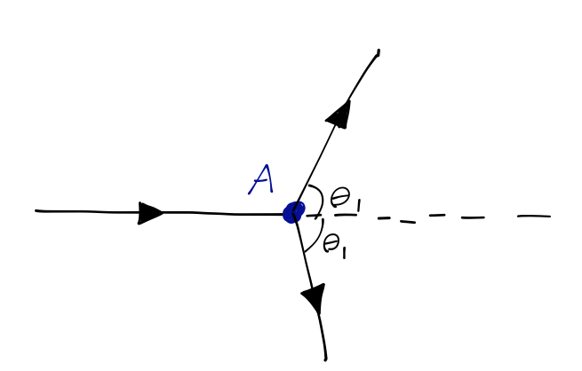
In this experiment, an incident beam of particles hits target A. We haven’t studied scattering theory in higher dimensions, but I will tell you that in this simple experiment, the intensity of the scattered beam is predicted to be dependent only on the angle \theta_1 between the incident and deflected beams in the beam-target plane. (This might not be completely obvious, but you can think of this as a version of the two-body problem in classical mechanics, where by symmetry we can consider the “orbits” as being confined to a plane containing the two objects.)

Now we introduce a pair of additional targets B and B', and we look for scattering in a second plane, which is tilted relative to the original scattering plane by an angle \phi. Once again, both classically or for quantum particles which don’t carry any spin, we find that the intensity of the doubly-scattered beam only depends on the angle \theta_2 in the second plane, and on the original angle \theta_1, but not on the relative orientation \phi of the two planes.
However, if the experiment is done with x-rays, then the outcome is very different. The x-ray intensity is observed to depend additionally on the orientation angle \phi, proportional to \cos^2 \phi. This is a polarization effect, and it’s consistent with our interpretation of light as a transverse propagating wave in the vector-valued \vec{E} and \vec{B} fields. The first scattering event polarizes the light in the beam-A plane, and then the amplitude to scatter again at B or B' depends on the projection of that polarization vector onto the new scattering plane, which goes as \cos \phi. Finally, the intensity is given by the squared amplitude, hence \cos^2 \phi.
Finally, we repeat the experiment with a beam of electrons, protons, neutrons, etc. This time, we find an intermediate result: the doubly-scattered beam intensity goes like \cos \phi. This is partly a surprise because it reveals that electron beams also exhibit some sort of polarization effect; they cannot be completely described by a scalar wavefunction \psi(\vec{x})! (This was true of light in the previous example too, incidentally.) But this is an even stranger result, because apparently the electron wavefunction can’t be represented by an ordinary vector, either; the linear dependence on \cos \phi means that the wavefunction, which we have to square to get the intensity, can’t be vector-valued (it is a spinor instead, as we know).