33 Scattering in three-dimensional systems
The one-dimensional S-matrix already has a rich structure, but the applications are a bit specialized; in the real world, we live in three spatial dimensions. As we will see, a significant amount of the physics that we observed in one dimension will transfer into this more realistic situation.
In one-dimensional scattering off of a fixed target of finite size, the S-matrix was a 2x2 object, since for a given scattering wave number k, the only adjustable parameter is whether our incoming wave from infinity comes from the left or from the right. But in three dimensions, in addition to choosing k, we can choose arbitrary spherical angles \theta and \phi to send a plane wave from. As with all of our previous work in three dimensions, rotational symmetry will be a very helpful tool to organize our approach.
Similar to how we began in one dimension, let’s consider the general situation of having a “black box” target region, this time taken to be a sphere of radius a around the origin:
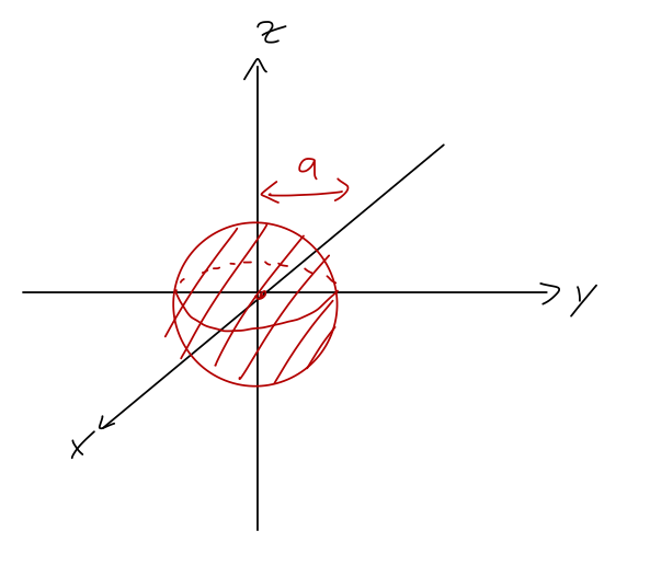
To begin with, we won’t make any strong assumptions about the black-box potential; in particular, we don’t assume that it necessarily has rotational symmetry. However, our solutions outside of the black box satisfy the free three-dimensional Schrödinger equation, so they do have full rotational symmetry, which means we can write them in the familiar form: \psi(\vec{r}) = \begin{cases} \sum_{l=0}^\infty \sum_{m=-l}^l R_{lm}(kr) Y_l^m(\theta, \phi), & r > a; \\ {\rm (unknown)}, & r \leq a; \end{cases} where the radial wavefunction now takes the form R_{lm}(kr) = A_{lm} h_l^{-}(kr) + B_{lm} h_l^{+}(kr). Here as usual \hbar k = \sqrt{2mE}, and h_l^{\pm}(u) are the spherical Hankel functions of the first (+) and second (-) kind, h_l^{\pm}(u) \equiv j_l(u) \pm i n_l(u), where j_l(u) and n_l(u) are spherical Bessel functions of the first and second kind. As discussed previously, there are some subtleties associated with boundary conditions at the origin and the spherical Bessel functions; since we’re covering the origin up with our “black box”, they don’t apply here and both Hankel functions are generally allowed for all l.
In our previous study of 3D wave mechanics, the radial part of the wavefunction had no dependence on m at all, \psi_{lm}(r) = R_{l}(kr) Y_l^m(\theta, \phi). This is because when we separated the radial and angular parts of the Schrödinger equation, the m dropped out of the radial equation completely. However, this separation relied on assuming rotational invariance of the potential, V(\vec{r}) = V(r).
While the external region where we’re writing our Hankel function solutions is free and thus rotationally invariant, at this point we’re not yet assuming the black box region is rotationally invariant. This means that while the free solutions themselves only depend on l, the boundary conditions that we can’t see at the black box can depend on m as well.
If we take the asymptotic limit r \rightarrow \infty, then the Hankel functions take on the approximate forms h_l^{\pm}(kr) \rightarrow \pm \frac{\exp(\pm i(kr - \tfrac{l\pi}{2}))}{ikr} In one dimension, we noted that Ae^{ikx} represented a “right-moving” wave, since if we add the time dependence back in it becomes Ae^{i(kx-\omega t)}, so the peak of the wave which occurs at x=0, t=0 translates to x=+(\omega t/k) at later times. If we do the same for the Hankel functions, we see:
- h_l^+ \sim \exp(i(kr - \omega t)) is an outgoing wave;
- h_l^- \sim \exp(-i(kr + \omega t)) is an incoming wave.
To better match on to the notation for our one-dimensional discussion, I’ve chosen A_{lm} as the amplitudes of the incoming waves.
33.1 Cross section
Now that we are in three dimensions and there are a continuous range of scattering directions, we can no longer capture the resulting physics simply in terms of reflection and transmission coefficients. Instead, we’ll frame things in terms of the scattering cross-section. It’s helpful to start by looking at how things are defined in the classical version of the scattering problem.
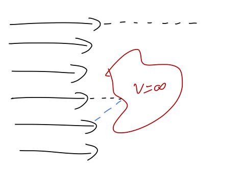
Suppose we have a classical target of some size, and a beam of classical particles that we will send in towards the target. To make it simple to think about, we consider a “hard” target, so that any individual particle will scatter if it intersects the target object, and otherwise will just fly past.
Of course, from just scattering one particle we don’t learn too much about our object. But suppose we throw a large number of particles N, in succession. Some number N_s of these will be scattered off, while the remaining N - N_s will just fly past. If we restrict our particles to a region of size A_B (the “beam area”), then clearly the number of scatters observed is related to the “cross-sectional area” A_T of the target object, \frac{N_s}{N} = \frac{A_T}{A_B}.
(If you’ve ever used certain Monte Carlo methods to calculate the volume of an object, then you’re familiar with this formula!) In this relation, A_T is an intrinsic property of our target, something we would like to determine from our experiment. On the other hand, the parameters A_B and N are adjustable properties of our scattering experiment. We can rearrange the ratio above as follows: N_s = A_T \frac{N}{A_B}. The combination N/A_B is an area density; it is, clearly, the figure of merit for how many scattering events we expect to see for a given beam experiment. If the target area is very small, we need this quantity to be very large to compensate, in order to get a reasonable number of scattered particles that we can detect.
The other requirement for a reasonable experiment is time: we don’t want to have to wait too long in order to find a scattering event. This means that it’s useful to consider the rate of scattering, \frac{dN_s}{dt} = A_T \frac{dN/dt}{A_B}. Thinking about the geometry of the problem, the number of particles on target per unit time is (on average) equal to the linear density along the direction of the beam, times the velocity of the particles, letting us rewrite: \frac{dN_s}{dt} = A_T \frac{v_B (N/L)}{A_B} = A_T v_B n_B, with n_B the number density of the beam, and v_B is the average velocity of the beam.
So far, all of this is purely classical, which means there are some fundamental limits on when it has a sensible interpretation; for example, we have assumed that the beam area is large, A_B > A_T, and the numbers N and N_s are integer numbers of scattering events. But using this classical story as inspiration, we define the following equation:
In a scattering experiment with a beam incident on a target, the scattering rate \Gamma_s satisfies the equation \Gamma_s \equiv \sigma \mathcal{L}, where \mathcal{L} is the instantaneous luminosity of the beam, the product of the beam number density times the average velocity, and \sigma is the cross section (units of area) which encodes the probability of interaction of the beam particles with the target.
There are two useful and common ways to rewrite this key expression. First, because the cross section is a property of the interaction and doesn’t depend on time, we can integrate both sides to obtain the number of scattering events, N_s = \sigma \left( \int dt\ \mathcal{L} \right), where the integral of \mathcal{L} is known as the integrated luminosity. If we have a target number of scattering events that we’d like to produce, this tells us how long we need to run our experiment to do so. Second, because the scattering direction is independent of the beam luminosity, we can take the differential of both sides with respect to solid angle: \frac{d\Gamma_s}{d\Omega} = \frac{d\sigma}{d\Omega} \mathcal{L}, and of course we can do both at once to relate dN_s/d\Omega to d\sigma/d\Omega. The quantity d\sigma/d\Omega is an example of a differential cross-section, here with respect to solid angle; it encodes how the interaction probability of our scattering events depends on the direction in which they are scattered, which we can then measure in the form of dN_s/d\Omega.
Strictly speaking, if we look at only the incoming beam of particles, the product of the beam number density times the average velocity is equal to the flux density, j (also with units of 1 / area / time.) Integrating this over the beam area A_B gives the flux, as a rate of number of scattering particles per second delivered to the target.
If we are talking about a single target, as in most of the discussion to follow here, then there is no difference between flux density and instantaneous luminosity. However, in most realistic experiments we are scattering from a target which has a large number of different identical particles in it; a sample of some material, or an oncoming beam of protons, for example. In these cases, the scattering rate depends on how likely we are to actually encounter one of the target atoms/particles/etc. in the target area. While the flux density only depends on our scattering beam, the luminosity is defined in order to take these other factors into account. In general, \mathcal{L} = j A_B n_T (\Delta x)_T or in words, the instantaneous luminosity is the total flux, times the number density of the target, times the thickness of the target. The dimensionful quantities cancel out, which is why flux density and luminosity have the same units, but the difference between the two definitions can be quite large!
33.2 The S-matrix in three dimensions
Here, I’ll rely on some nice lecture notes on partial waves from Y.D. Chong, especially for some details of how to write things out in the general case without full rotational symmetry.
As in our one-dimensional example, we’ll define the S matrix as the object that relates the outgoing amplitudes to the incoming amplitudes. For a fixed value of l and m, we have only one incoming and one outgoing wave; however, without imposing rotational symmetry any (l,m) can scatter into any (l', m'). Let’s use the shorthand notation \mu \equiv (l,m), referring to the label \mu as a “scattering channel”, a label which uniquely identifies a single incoming or outgoing state. In this notation, the S-matrix is defined as B_{\mu} = \sum_{\nu} S_{\mu \nu} A_{\nu} matching the matrix-vector notation we used in one dimension (where there were always two scattering channels, “left” and “right” or “parity-even” and “parity-odd”.) In three dimensions the number of scattering channels is formally infinite. Our particular choice of scattering channels (i.e. choice of basis) here, using the spherical harmonics, is known as partial wave expansion.
Like the parity basis in one dimension, the use of the partial wave basis has especially nice properties and results in a simpler S-matrix, particularly if we impose more symmetries like rotational invariance. Also like the parity basis, the incoming states aren’t especially simple to realize in an experiment. Typically, a real scattering experiment would involve something more like an incoming plane wave from a certain direction. To map between the two, we can derive a simple identity to write a plane wave in terms of spherical harmonics:
A plane wave of the form e^{i\vec{k} \cdot \vec{r}} can be expanded in partial waves (see these notes for a nice derivation) as e^{i\vec{k} \cdot \vec{r}} = 4\pi \sum_{l=0}^\infty \sum_{m=-l}^l i^l j_l(kr) (Y_l^m)^\star(\hat{k}) Y_{l}^m(\hat{r}) with the spherical harmonics evaluated at spherical angles corresponding to the directions of \vec{k} and \vec{r}.
For the special case where \vec{k} is chosen to be in the positive z direction, we have the simpler result e^{ikr \cos \theta} = \sum_{l=0}^\infty i^l (2l+1) j_l(kr) P_l(\cos \theta). This removes the \phi dependence since those correspond to rotations around the beam direction; however, the scattered wave will still depend on \phi unless the target is rotationally symmetric.
It’s worth noting that although we would like to think of it as purely “incoming” to the target, the plane-wave solution clearly has both incoming and outgoing components in terms of the spherical basis, since 2 j_l(kr) = h_l^+(kr) + h_l^-(kr). This doesn’t change anything with respect to the definition of the S-matrix, but we can separate each outgoing amplitude B_{\mu} into two parts, B_\mu = B_\mu^i + B_\mu^s, one from the incoming plane wave and one from the scattering off of the potential. From our result above, we can read off the expressions for the incoming and outgoing partial-wave amplitudes, which will be useful later: A_{lm} = B_{lm}^{i} = 2\pi \mathcal{N} i^l (Y_l^m)^\star(\hat{k}), where \mathcal{N} is the normalizing constant for the incoming plane wave.
33.2.1 Symmetry and the 3D S-matrix
I won’t go as deep into symmetry constraints on the S-matrix here as we did in one dimension, but two very important remarks are in order. First, an important and very general constraint to impose is conservation of probability flux. Although I won’t include the derivation here, one can prove that the consequence of probability conservation is the same as in one dimension, that the S-matrix is unitary: S^\dagger S = 1.
Second, while I have set things up in the most general case, from here forward we will focus on the case where the “black box” is spherically symmetric. If this is true, then the full potential is spherically symmetric everywhere, which guarantees conservation of angular momentum. This has the obvious consequence that scattering can no longer change the angular momentum quantum numbers of an incoming spherical wave, which means the S matrix becomes diagonal: S_{l'm', lm} \rightarrow S_l \delta_{ll'} \delta_{mm'}.
If we combine the properties of being diagonal and unitary, then we see that with rotational symmetry all entries of the S-matrix must further satisfy |S_{l}|^2 = 1, which means that they are pure phases, S_l = e^{2i\delta_l}. (The factor of two is a standard convention.) Physically, this tells us that due to angular momentum conservation, the probability flux is conserved within each partial wave, |A_l|^2 = |B_l|^2; in other words, the probability to find a particle with angular momentum l is the same for incoming vs. outgoing.
33.3 Scattering amplitude
Now that we’ve defined what we’re looking for more properly, let’s go back to the quantum scattering case and relate the cross section to the S-matrix. In general, this can be done by using probability currents. As a quick reminder, the general definition is \vec{j} = \frac{\hbar}{m} \textrm{Im} (\psi^\star \nabla \psi). What are the units of the probability current? In three dimensions, we recall that normalization \int d^3x |\psi|^2 = 1 tells us that \psi has units of [L]^{-3/2}. The gradient gives another power of 1/[L], while from \hbar/m we get [L]^2/[T]. So the overall result is [\vec{j}] = \frac{1}{[L]^2 [T]} which is the same units as instantaneous luminosity, \mathcal{L}. This shouldn’t be a surprise; we already pointed out that \mathcal{L} has units of flux density, and \vec{j} is certainly a flux density. More specifically, in single-target quantum scattering, the incoming flux density |\vec{j}_{\rm in}| = \mathcal{L}.
We can similarly calculate the flux density of the outgoing wave, \vec{j}_{\rm scatter}, from the scattering part of the total wavefunction. Outgoing flux wasn’t quite how we phrased things in our cross-section discussion above, but we can make contact by taking an infinitesimal area dA = r^2 d\Omega somewhere outside the target and measuring the flux passing through it; you can think of this as representing the need for a detector of size dA to measure the outgoing wave. Integrating flux times area gives us a rate, which is exactly the differential scattering rate: \frac{d\Gamma_s}{d\Omega} = \int d\vec{A} \cdot \vec{j}_{\rm scatter}. (where the vector on d\vec{A} orients the tiny area we’re looking at.) Dividing out the luminosity |\vec{j}_{\rm in}| gives us the cross section d\sigma/d\Omega.
This gives us a general roadmap for what to do: the S-matrix gives us the relation between incoming and outgoing components of the exterior wavefunction \psi. From \psi, we can calculate the probability currents \vec{j}_{\rm in} and \vec{j}_{\rm scatter}. This gives us the luminosity, the rate, and the cross section as above.
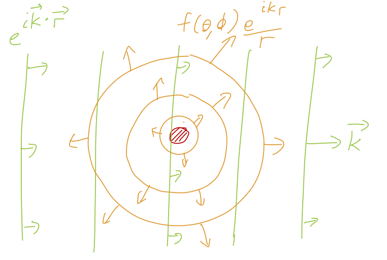
While this recipe is fairly general, to get nicer formulas I’m going to specialize now to the case of an incoming plane wave. Since we’re free to choose the axis of the plane wave, we’ll select it to be moving along the z axis in the positive direction in order to define our angular coordinates. Imposing conservation of probability here will let us find a very specific form for the wavefunction \psi; I’m going to start by skipping you the answer and giving you some physical intuition about it. Here are the key result and a sketch of what is happening:
Given an incident plane wave scattering off a target at the origin, so that the overall form of the wavefunction is (asymptotically and neglecting the overall normalization) \psi(\vec{r}) = e^{i\vec{k} \cdot \vec{r}} + f(\theta, \phi, k) \frac{e^{ikr}}{r}, where the function f(\theta, \phi, k) (sometimes written just as f(\theta, \phi) with k-dependence implicit) is known as the scattering amplitude. The spherical angles \theta, \phi are defined with respect to the incoming beam axis defined by \vec{k}.
From this wavefunction, the differential scattering cross section is given by \frac{d\sigma}{d\Omega} = |f(\theta, \phi)|^2.
The physical picture here is as follows: our incoming plane wave hits and also passes through the target, setting the incoming amplitudes A_\mu and part of the outgoing amplitudes B_\mu^i as discussed above. The remaining outgoing amplitude B_\mu^s is from the scattered wave off the target. Conservation of probability requires the scattered wave to be of the form e^{ikr}/r times the scattering amplitude. The 1/r dependence is due to the fact that the scattered particles are spreading out over the surface of an ever-larger sphere as r increases, so the local flux must decrease with r.
Because our incoming plane wave gives some flux just passing through the target, we do have to be careful to separate out the scattering part. The total outgoing spherical wave can be decomposed as B_\mu = \sum_\nu S_{\mu \nu} A_\nu If we write B_\mu = B_\mu^i + B_\mu^s for the two components, then we can use the fact that A_\mu = B_\mu^i to write B_\mu^s = \sum_\nu \left[ S_{\mu \nu} - \delta_{\mu \nu} \right] A_\nu Physically, to isolate the scattering modes that have actually interacted with the target, we need to subtract off the part of the incoming plane wave that just passes through the target. By convention, we define the T-matrix as S \equiv 1 + iT which just contains the interacting part of the S-matrix. The scattering amplitude is then B_\mu^s = i \sum_\nu T_{\mu \nu} A_\nu.
For a plane wave, we readily find the result \vec{j}_{\rm in} = \frac{\hbar k}{m} |\mathcal{N}|^2 \hat{k}, with \mathcal{N} the normalization of the plane-wave state and \hat{k} = \vec{k} / k.
As a reminder, plane waves are an idealization which have some mildly unphysical properties, most notably that they can’t be normalized properly in an infinite volume. The best interpretation of a plane wave, which is also the one which happens to be most useful in the present context, is as a representation of a steady-state beam of particles. With this interpretation, we’ll be able to absorb the unphysical normalization factor into how we define incoming particle flux and it won’t appear in our final answers.
Restoring the full functional form from above, the total scattered part of the wavefunction is thus \psi^s(\vec{r}) = \sum_{l=0}^\infty \sum_{m=-l}^l B_{lm}^s h_l^{+}(kr) Y_l^m(\theta, \phi). To find the current, we need to take a gradient, but we really don’t want to evaluate the gradient of an arbitrary spherical Hankel function. Instead of attacking this directly, let’s remember that we’re doing a scattering experiment, which means what we really care about is the value of the current at very large r, where we will detect it. Thus, we can use the asymptotic form, h_l^{+}(kr) \approx \frac{\exp\left( i(kr - l\pi/2) \right)}{ikr} = i^{-(l+1)} \frac{e^{ikr}}{kr} + \mathcal{O}(\frac{1}{r^2}). So the asymptotic functional form is the same for all h_l^{+}(kr), with just the phase changing with l. This means that the gradient is, also asymptotically, \nabla h_l^{+}(kr) \approx i^{-l} \frac{e^{ikr}}{r} \hat{r} + \mathcal{O}\left(\frac{1}{r^2}\right) = ikh_l^{+}(kr) \hat{r}. For our wavefunction, notice that if apply the asymptotic expansion first, we can pull the radial dependence out of the sum completely: \psi^s(\vec{r}) \rightarrow \frac{e^{ikr}}{r} \sum_{l=0}^\infty \sum_{m=-l}^l B_{lm}^s \frac{i^{-(l+1)}}{k} Y_l^m(\theta, \phi) \\ \equiv \frac{e^{ikr}}{r} \mathcal{N} f(\theta, \phi, k) where f(\theta, \phi, k), which only depends on the incident energy and the scattering angle, is known as the scattering amplitude. (I’ve also pulled out a factor of the normalization of the incoming plane wave, which will cancel out soon.) This means that for the combination of terms in the probability current, (\psi^s)^\star \nabla \psi^s = \frac{e^{-ikr}}{r} \mathcal{N}^\star f^\star(\theta, \phi) \left[ ik\frac{e^{ikr}}{r} \mathcal{N} f(\theta, \phi) \hat{r} + \frac{e^{ikr}}{r} \mathcal{N} \nabla f(\theta, \phi) \right] \\ \approx \frac{k}{r^2} |\mathcal{N}|^2 \left[ i|f(\theta, \phi)|^2 \hat{r} \right] + \mathcal{O} \left( \frac{1}{r^3} \right), where I’m relying one more time on the asymptotic expansion to discard the gradient \nabla f; since f is purely a function of angles, the surviving terms in the gradient in spherical coordinates all come with at least a factor of 1/r, so in the leading asymptotic expansion we should simply ignore it. Putting the pieces together, we have for the scattering current \vec{j}_{\rm scatter} \approx \frac{\hbar k}{m} |\mathcal{N}|^2 \frac{1}{r^2} |f(\theta, \phi, k)|^2 \hat{r}. While the incoming current is constant, the scattering current dies off as 1/r^2. This is just what we expect, since the incoming beam is unidirectional but the scattered particles are spreading out over the surface of an ever-larger sphere as r increases. To convert this into a scattering rate, we should integrate it over some area; we’ll take an infinitesimal chunk of the scattering sphere of area dA = r^2 d\Omega (this could represent the area of our detector.) Then we have for the rate through this area \frac{d\Gamma_{s}}{d\Omega} = \frac{\hbar k}{m} |\mathcal{N}|^2 |f(\theta, \phi, k)|^2. But |\mathcal{N}|^2 \hbar k/m is exactly the incoming flux \vec{j}_{\rm in}, which is also the instantaneous luminosity \mathcal{L}, as we observed in the general case above. So by inspection, we find the key result given above, that \frac{d\sigma}{d\Omega} = |f(\theta, \phi, k)|^2.
Notice how beautiful and simple this is; in particular, with the way that cross section is defined, this formula holds no matter what the parameters of the beam are. It only depends on the energy and direction of the beam, as determined by the wave vector \vec{k}.
To finish things out, we finally need to define how to relate the scattering amplitude f(\theta, \phi, k) to the S-matrix. By definition from above, we see that f(\theta, \phi, k) = \frac{1}{\mathcal{N}} \sum_{l,m} B_{lm}^s \frac{i^{-(l+1)}}{k} Y_l^m(\theta, \phi) = \sum_{l,m} \left[ \sum_{l',m'} (T_{lm;l'm'} \frac{1}{\mathcal{N}} A_{l'm'}) \right] \frac{i^{-l}}{k} Y_l^m(\theta, \phi) We can go further by recalling that we know the form of the A_{lm} coefficients for a plane wave; substituting in from above gives (for a wave incident in the \vec{k} direction), f(\theta, \phi) = \sum_{l,m} \sum_{l',m'} T_{lm;l'm'} \frac{1}{\mathcal{N}} (2\pi \mathcal{N} i^{l'} (Y_{l'}^{m'})^\star(\hat{k})) \frac{i^{-l}}{k} Y_l^m(\theta, \phi).
Simplifying a bit, we have the final scattering amplitude result in the box just below.
The remaining piece of the puzzle we need to get physics out is to know how the scattering amplitude f(\theta, \phi) is related to the S-matrix. If we go through the detailed algebra covering conservation of probability flux that I’ve hidden as an aside above, the answer drops out:
Given a scattering target potential which is not assumed to be spherically symmetric, the scattering amplitude for an incoming plane-wave beam with wave vector \vec{k} is given in terms of the T-matrix, related to the S-matrix as S = 1 + iT, by the formula f(\theta, \phi)= \frac{2\pi}{k} \sum_{l,m} \sum_{l',m'} T_{lm;l'm'} i^{(l'-l)} (Y_{l'}^{m'})^\star(\hat{k}) Y_l^m(\theta, \phi).
The problem with the general case for 3d scattering is that the S-matrix is both infinite and dense (i.e. has many non-zero entries), so general scattering problems without spherical symmetry are very difficult and often best solved numerically. I wanted to get you this far in case you need to work with such a problem in the future, but to see the remaining interesting physics in scattering theory without so much calculational overhead, from here forward we’ll specialize to the spherically symmetric case.
33.4 Scattering with spherical symmetry
As we noted above, an immediate consequence of spherical symmetry is that the S-matrix becomes fully diagonal in the angular momentum quantum numbers, S_{l'm',lm} \rightarrow e^{2i\delta_l} \delta_{ll'} \delta_{mm'}. This collapses the T-matrix similarly, which means that each scattered wave component B_{lm}^{s} is given simply from the incoming A_{lm} in terms of a single phase shift \delta_l.
Since we are assuming spherical symmetry, it is even more expedient to exploit it immediately and force our beam axis to be the +z axis without any loss of generality (for a spherically symmetry target, all incoming axes are equivalent.) For collapsing spherical harmonics, we can invoke the useful identities Y_l^0(\theta, \phi) = \sqrt{\frac{2l+1}{4\pi}} P_l(\cos \theta) \\ Y_l^m(0, \phi) \propto \delta_{m0} and for the harmonic Y_{l}^{m}(\hat{k}) corresponding to the beam direction, P_l(\cos \theta_k) = P_l(1) = 1 for any l. This gives us a simpler expression for the scattering amplitude in terms of the phase shifts, and removes the \phi dependence and the m dependence completely. Using these identities in the general scattering amplitude formula above, we have:
Given a scattering target potential which is spherically symmetric, the scattering amplitude for an incoming plane-wave beam with wave vector \vec{k} (taken to be in the +z direction) is given in terms of the scattering phase shifts (determined from the S-matrix by S_l = e^{2i\delta_l}) by the formula f(\theta) = \frac{1}{2ik} \sum_{l=0}^\infty (e^{2i\delta_l}-1) (2l+1) P_l(\cos \theta) \\ = \sum_{l=0}^\infty (2l+1) f_l P_l(\cos \theta), defining the partial wave amplitudes conventionally as f_l(k) \equiv \frac{e^{2i\delta_l} - 1}{2ik}.
With spherical symmetry, the partial-wave phase shifts \delta_l are the key objects containing all the physics. It’s often useful to write the wavefunction directly in terms of the phase shifts by eliminating B_l: we see that R_l(r) = A_l h_l^-(kr) + B_l h_l^+(kr) = A_l [h_l^-(kr) + e^{2i\delta_l} h_l^+(kr)] or converting back to spherical Bessel functions, R_l(r) = A_l [(e^{2i\delta_l}+1) j_l(kr) + (e^{2i\delta_l} - 1)in_l(kr)] \\ = 2A_l e^{i\delta_l} [ \cos (\delta_l) j_l(kr) - \sin (\delta_l) n_l(kr) ].
There are a few equivalent expressions for the partial-wave amplitudes that you will see in the literature which are useful to know: it’s easy to verify that
f_l(k) = \frac{e^{2i\delta_l} - 1}{2ik} = \frac{e^{i\delta_l} \sin \delta_l}{k} = \frac{1}{k \cot \delta_l - ik}.
Show that all three expressions for f_l(k) given above are indeed the same thing.
Answer:
(to be filled in!)
33.4.1 Optical theorem and partial waves
Let’s have a look at the cross section based on this simplified version of the amplitude. We have \frac{d\sigma}{d\Omega} = |f(\theta)|^2 \\ = \frac{1}{4k^2} \sum_{l,l'} (2l+1) (2l'+1) (e^{-2i\delta_{l'}}-1)(e^{2i\delta_{l}}-1) P_{l'}(\cos \theta) P_{l}(\cos \theta) This isn’t especially illuminating yet, but if we integrate over the solid angle to get the total cross section, we can use an orthogonality relation between the Legendre polynomials, \int_{-1}^1 du P_l(u) P_{l'}(u) = \frac{2}{2l+1} \delta_{ll'} to find that \sigma = \int d\Omega \frac{d\sigma}{d\Omega} = 2\pi \int_{-1}^1 d(\cos \theta) |f(\theta)|^2 \\ = \frac{\pi}{k^2} \sum_l (2l+1) |e^{-2i\delta_{l}}-1|^2 \\ = \frac{4\pi}{k^2} \sum_l (2l+1) \sin^2 \delta_l. The first important thing we see from this derivation is that the total cross-section itself can be defined as a sum over partial wave cross-sections, \sigma = \sum_l \sigma_l, where we have defined \sigma_l = \frac{4\pi}{k^2} (2l+1) \sin^2 \delta_l = 4\pi (2l+1) |f_l(k)|^2. This immediately gives us a powerful constraint which is independent of our physical system, since \sin^2 \delta_l \leq 1:
For scattering in a system with spherical symmetry, the partial-wave cross section for a given angular momentum channel l must satisfy the bound \sigma_l \leq \frac{4\pi}{k^2} (2l+1).
This is known as a “unitarity bound” since violation of the bound can be related to scattering of particles in the given channel having a probability greater than 100%. (More indirectly, it arises from being able to characterize the S-matrix completely with a phase shift, which required S-matrix unitarity to get to.)
Going back to the total cross section, there is another useful result if we compare to the scattering amplitude in the beam direction (also known as the “forward” direction), at \theta = 0: f(0) = \frac{1}{2ik} \sum_l (e^{2i\delta_l} - 1) (2l+1) \\ = \frac{1}{k} \sum_l (2l+1) e^{i\delta_l} \frac{1}{2i} (e^{i\delta_l} - e^{-i\delta_l}) \\ = \frac{1}{k} \sum_l (2l+1) e^{i\delta_l} \sin \delta_l
This is close to the result for the total cross section, which leads to the following result:
For scattering in a system with spherical symmetry, the total cross section \sigma is related to the forward scattering amplitude f(0) as \sigma = \frac{4\pi}{k} {\rm Im}[f(0)].
The optical theorem is not a purely quantum phenomenon, since it holds much more generally for scattering of waves, including classical waves (it was first derived in the context of optics, hence the name.) The optical theorem is useful and powerful but is also not a very intuitive statement in my opinion, especially since the way that we arrived at it was simply to notice a mathematical equivalence between two expressions instead of working through any deeper principle. To try to give at least a little intuition, here are a few observations that might help:
In the trivial case where there is no target (\sigma = 0), the optical theorem says that the imaginary part of f(0) = 0. This is sort of trivial, since if there is no scatterer then the entire T-matrix is zero, all phase shifts \delta_l = 0, and therefore f(0) = 0 (the real part vanishes too.)
Although I won’t attempt to do it because the derivation is a little technical, if we consider the full asymptotic wavefunction \psi(r) = e^{ikr \cos \theta} + f(\theta) \frac{e^{ikr}}{r} and ask what the flux is in the forward direction, we find that it’s equal to the incoming flux reduced by the amount (4\pi/k) {\rm Im}[f(0)]. In other words, the imaginary part of the forward amplitude gives the amount of particles that are scattered away from forward. The optical theorem then becomes a statement of conservation of probability; the amount of flux scattered away from the forward direction is equal to the amount of stuff measured in all other directions (given by \sigma.)
When we use something like perturbation theory to compute the scattering amplitude, we can encounter apparent violations of the optical theorem. This follows simply from the fact that if we expand e^{i\delta} \approx 1 + i\delta - \delta^2/2 + ..., then at finite order in our expansion it’s no longer true that e^{i\delta} e^{-i\delta} = 1. This is an apparent violation of unitarity, but it’s a mirage of our expansion: the optical theorem is an exact and non-perturbative statement. Moreover, it can provide a useful check on perturbative calculations, since the amplitude will “unitarize” (come closer to satisfying the optical theorem) order by order in whatever expansion we use.
33.4.2 Example: Quantum hard-sphere scattering
Let’s do a concrete example, starting with the simplest case of a hard sphere: V(r) = \begin{cases} \infty, &r \leq a; \\ 0, &r > a. \end{cases} Since there is no interior region, we already have the complete wavefunction: \psi(\vec{r}) = \begin{cases} 0, & r \leq a; \\ \sum_{l=0}^\infty R_{l}(kr) \sum_{m=-l}^l Y_l^m(\theta, \phi), & r > a; \end{cases} and we’ll use the form with the phase shift in it from above, R_l(kr) = 2A_l e^{i\delta_l} [ \cos (\delta_l) j_l(kr) - \sin (\delta_l) n_l(kr) ]. The boundary condition at the infinite barrier requires that R_l(ka) = 0, from which we can read off the condition \tan (\delta_l) = \frac{j_l(ka)}{n_l(ka)}. This is especially simple for the s-wave: if l=0, then using j_0(\rho) = \sin \rho / \rho and n_0(\rho) = -\cos \rho/\rho, we read off that \delta_0 = -ka. For larger l we have to resort to numerics quickly, but there are some interesting things we can look at. First of all, if the scattering is very high-energy, the asymptotic forms of the spherical Bessel functions give us k \rightarrow \infty:\ \ \tan (\delta_l) \rightarrow \frac{\sin(ka - \tfrac{l\pi}{2})}{-\cos(ka - \tfrac{l\pi}{2})}. which gives us the same simple result plus an extra l-dependent phase shift, \delta_l \approx -ka + \frac{l\pi}{2}. However, it’s important to note that this asymptotic form has a caveat: it only works if the argument of Bessel function is much larger than l, i.e. we must have l \lesssim ka. We can make a physics argument that there is a maximum possible l value for high-energy scattering anyways. Recall that one way to think of the spherically-symmetric three-dimensional Schrödinger equation is by rewriting it as a one-dimensional problem for rR_{El}(r), with “effective potential” including a centrifugal barrier V_{\rm eff}(r) = V(r) + \frac{\hbar^2 l(l+1)}{2mr^2} = V(r) + V_{\rm cf}(r).
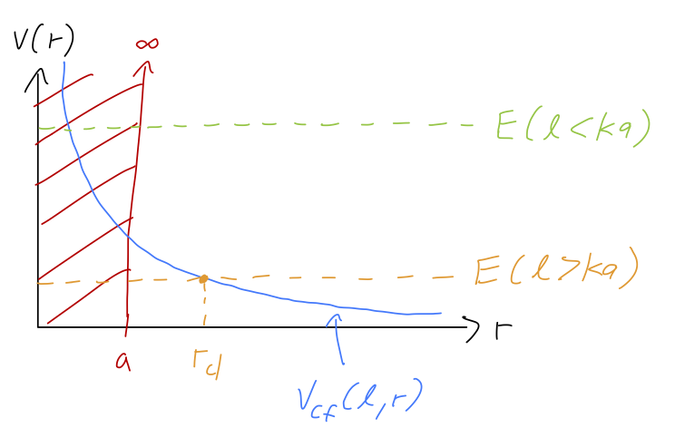
For any given value of the energy, if l is large enough, the centrifugal barrier repels our particle from the origin - meaning in our scattering experiment that we never reach r=a to make contact with the sphere. In fact, we can see that the classical turning point with zero potential (outside the hard sphere) is r_{\rm cl} = \sqrt{\frac{\hbar^2 l(l+1)}{2mE}} \sim \frac{l}{k} so we see that if l > ka, then classically our particle just flies past the target. Of course quantum mechanically, there is still some overlap with the hard sphere boundary even for l just above ka, but we expect (and would find from a careful treatment of the spherical Bessel functions) that the phase shifts will drop rapidly to zero as l increases beyond ka.
This is enough for us to compute the total cross section for high-energy scattering: \sigma(k \rightarrow \infty) = \frac{4\pi}{k^2} \sum_l (2l+1) \sin^2 \delta_l \\ \approx \frac{4\pi}{k^2} \sum_{l=0}^{l_{\rm max}} (2l+1) \sin^2 \left( ka - \frac{l\pi}{2} \right) \\ \approx \frac{4\pi}{k^2} \int_0^{ka} dl\ (2l+1) \sin^2 \left(ka - \frac{l\pi}{2} \right) Since l is very large, we can replace (2l+1) with (2l) and also replace the \sin^2 with its average value of 1/2 since it’s oscillating very rapidly, leaving the result \sigma(k \rightarrow \infty) \approx \frac{4\pi}{k^2} \frac{(ka)^2}{2} = 2\pi a^2. This is exactly a factor of 2 larger than the classical cross section (which is just the cross-sectional area of the sphere, \pi a^2); there is a remnant of quantum behavior even in the high-energy limit, which is related to the presence of forward scattering at \theta = 0 which is always present as per the optical theorem. (This gives a “bright spot” in the forward direction at \theta = 0, whereas in the fully classical particle-scattering case, there is a perfect shadow behind the hard sphere so the forward rate is zero.)
The low-energy limit E \rightarrow 0 is also interesting to look at. This implies that ka \ll 1, which we can use to invoke the small-\rho behavior of the spherical Bessel functions, immediately giving the result k \rightarrow 0:\ \ \tan \delta_l \rightarrow \frac{-(ka)^{2l+1}}{(2l+1)!!(2l-1)!!} In addition to the double-factorial suppression, we see that every increase in l is also suppressed by another power of (ka)^2. This means that the scattering cross-section will be dominated completely by the s-wave piece: \sigma \approx \sigma_0 = \frac{4\pi}{k^2} \sin^2 \delta_0 \approx \frac{4\pi}{k^2} (-ka)^2 = 4\pi a^2. Here we find a result which is a factor of 4 larger than the classical cross-sectional area. Since in the small-energy limit our incoming particles are highly wave-like and non-classical, it isn’t too surprising that we get something different from the classical area.
Finally, we could try to look at the structure of the phase shifts in the complex plane - but we won’t find anything interesting in this case. There are no solutions with E < 0 and thus no bound states, and we also won’t find any transmission resonances; if you sketch the effective one-dimensional potential this will be obvious, since it’s just monotonically increasing until we hit either the wall at r=a or the classical turning point.
33.5 Universality of low-energy scattering
Let’s zoom back out to the more general picture of (spherically symmetric) scattering. For the hard sphere example, at low energy ka \ll 1 we found that the phase shifts decreased rapidly as l increased, leading to complete dominance of the cross section by the l=0 (s-wave) contribution. A natural question is: can we generalize statements about the k dependence of the phase shifts to more general potentials V(r)?
To consider this question, let’s use the form of the exterior radial wavefunction in terms of phase shifts that we found above. Since we’re assuming spherical symmetry, we can ignore all angular dependence and just focus on the radial wavefunction, which for the full problem is R(r) = \begin{cases} R_l^{<}(r), & r \leq R; \\ R_l^{>}(r) = 2A_l e^{i\delta_l} \left[ \cos (\delta_l) j_l(kr) - \sin (\delta_l) n_l(kr) \right], & r > R. \end{cases} (I have switched from a to R for the boundary value of the radius, to avoid notational confusion below.) At r=R, we have to match a boundary condition between our solutions; but we have to be careful, since even if we ignore \theta and \phi this is still a three-dimensional problem! We discussed radial boundary conditions a bit back in our first encounter with 3d wave mechanics in Chapter 12, but as a reminder, for matching at a general boundary like this the condition takes the form \left. \frac{1}{R_1} \frac{dR_1}{dr} \right|_{r=R} = \left. \frac{1}{R_2} \frac{dR_2}{dr} \right|_{r=R} Both sides can also be written as d(\log R_i)/dr, so this condition is sometimes referred to as “continuity of the logarithmic derivative”. Now, since we’re considering the general case we don’t know what the interior solution R_l^<(r) is, but we can use it to define the quantity \beta_l \equiv \left. \frac{r}{R_l^<} \frac{dR_l^<}{dr} \right|_{r=R} adding the r to make this quantity dimensionless. For the exterior solution, we can calculate this: \beta_l = kR \frac{\cos (\delta_l) j_l'(kR) - \sin(\delta_l) n_l'(kR)}{\cos (\delta_l) j_l(kR) - \sin(\delta_l) n_l(kR)} which can be solved for the phase shift, in the form \tan \delta_l = \frac{j_l(kR)}{n_l(kR)} \left[ \frac{kR (j_l'(kR) / j_l(kR)) - \beta_l}{kR (n_l'(kR) / n_l(kR)) - \beta_l} \right]. If we know the form of the interior solutions so we can compute \beta_l, then this form immediately gives us the phase shifts and thus the solution to the scattering problem, so this is a useful expression on its own. (Note that we recover our previous simple result for the hard sphere if we take \beta_l \rightarrow \infty for all l, corresponding to the wavefunction vanishing suddenly at the infinite barrier.) But now, we can use it to consider what happens in some limiting cases. Trying to take k \rightarrow \infty isn’t very illuminating; as we saw in the hard-sphere case there is some delicate interplay with the value of l, and generally the results in this limit depend very strongly on the unknown interior potential.
On the other hand, the k \rightarrow 0 limit is more revealing. Recalling the asymptotic forms of the spherical Bessel functions in this limit, j_l(\rho) \approx \frac{\rho^l}{(2l+1)!!}, \\ n_l(\rho) \approx -\frac{(2l-1)!!}{\rho^{l+1}}, we see first of all that the ratios of derivatives are j_l'(\rho) / j_l(\rho) = l/\rho, \\ n_l'(\rho) / n_l(\rho) = -(l+1) /\rho, and the ratio j_l(\rho)/n_l(\rho) we already computed above in this limit. Putting things together, we see that \tan \delta_l \approx \frac{-(kR)^{2l+1}}{(2l+1)!!(2l-1)!!} \left[ \frac{l-\beta_l}{-(l+1)-\beta_l} \right].
Note that in general \beta_l itself is not just a constant; it depends implicitly on both k and on R. However, due to the way it enters into this expression for the phase shift, the leading behavior at small k of the quantity in square brackets has to be constant if we expand for small kR, so that it won’t change the leading kR dependence.
In the low energy limit defined as kR \rightarrow 0, with R the size of the scattering target, the leading behavior of the scattering phase shifts for an arbitrary spherically-symmetric potential is \tan \delta_l \sim (kR)^{2l+1}.
On physical grounds, we can also argue generally that at small k, the potential energy dominates over other terms inside of the potential well, and so \beta_l will be approximately k-independent. There is a beautiful 1949 result by Hans Bethe on studying nuclear potentials which argues for ignoring the k dependence of \beta_l and arrives at the simple two-parameter model we will introduce below, to which I refer you for more details.
33.5.1 Scattering length and effective range
Because the leading dependence of \tan \delta_l goes as (kR)^{2l+1}, one important conclusion we can draw immediately is that in terms of the total cross section, the l=0 s-wave phase shift will be entirely dominant. Since the form of the spherical Bessel functions is especially simple for the s-wave, we can back up a step and do a slightly more general expansion. Recalling that j_0(\rho) = \sin \rho / \rho and n_0(\rho) = -\cos \rho / \rho, the derivative ratios simplify to j_0'(\rho) / j_0(\rho) = \cot (\rho) - \frac{1}{\rho}, \\ n_0'(\rho) / n_0(\rho) = -\tan (\rho) - \frac{1}{\rho}.
Going back to our formula for the phase shift, then, we find \tan \delta_0 = -\tan (kR) \left[ \frac{kR \cot (kR) - 1 - \beta_0}{-kR \tan (kR) - 1 - \beta_0 } \right] \\ = - \frac{kR - (1+\beta_0) \tan (kR) }{(1 + \beta_0) + kR \tan (kR)}. This is an exact expression for the s-wave phase shift, if we know \beta_0. But let’s assume \beta_0 is independent of k and then series expand in kR \ll 1: the series expansion of tangent is \tan u \approx u + u^3/3, so we find \tan \delta_0 \approx - \frac{kR - (1+\beta_0) (kR + (kR)^3/3)}{(1+\beta_0) + kR (kR + (kR)^3/3)} \\ \approx \frac{kR}{1+\beta_0} \left( \beta_0 + (1+\beta_0) (kR)^2/3 \right) \left(1 - \frac{(kR)^2}{1+\beta_0} \right) \\ = kR \left( \frac{\beta_0}{1+\beta_0} \right) + (kR)^3 \left( \frac{1}{3} - \frac{\beta_0}{(1+\beta_0)^2} \right) + ... This determines a pair of constants that determine the leading and subleading dependence of the s-wave phase shift, and therefore of the cross section. We can rewrite them in a more conventional form:
For s-wave scattering in the limit of low energy, the scattering phase shift is approximately given by the equation k \cot \delta_0 \approx -\frac{1}{a_0} + \frac{1}{2} r_0 k^2 + ... where a_0 is known as the scattering length, and r_0 is known as the effective range. Both constants have units of length, and depend on the properties of the target potential.
If desired we can find formulas for both in terms of \beta_0 by rearranging and re-expanding our result above, but in practice it’s often simpler just to solve for \cot \delta_0 and then series expand directly.
We can plug back in to find the s-wave cross section, which is approximately the total cross section, in terms of these two parameters: \sigma \approx \sigma_0 = 4\pi |f_0(k)|^2 \\ = \frac{4\pi}{|k \cot \delta_0 - ik|^2} \\ \approx \frac{4\pi}{|-1/a_0 + \tfrac{1}{2} r_0 k^2 - ik|^2} \\ = \frac{4\pi a_0^2}{1 + (1 - r_0/a_0) k^2 a_0^2} + \mathcal{O}(k^4). (Note that since \cot \delta_1 \sim 1/k^3, the lowest order p-wave contribution to the cross section is included in the k^4 term, which is why keeping the effective range but not \delta_1 is a sensible thing to do.)
In the limit that k \rightarrow 0, we recover the cross-section as 4\pi a_0^2. In the hard-sphere scattering case we can read off that a_0 is just the radius of the sphere, and we recover the “geometric” cross section.
The universal behavior that we have uncovered allows us to make simple but useful statements about arbitrary scattering potentials. Although only a_0^2 determines the cross section, the scattering length a_0 itself can be either positive or negative. It turns out that repulsive potentials (e.g. barriers with V_0 > 0) tend to give a positive scattering length; if we compute it for the hard sphere, we will find a_0 = R. This corresponds to the free wavefunction being “pushed out” from the origin by the repulsive force. Similarly, a negative scattering length tends to be associated with an attractive potential (although potential wells can also give positive scattering lengths.)
A particularly interesting physics system for which our current discussion is very relevant is the study of Bose-Einstein condensates (BECs). A Bose-Einstein condensate of neutral atoms is extremely dilute and extremely cold: the de Broglie wavelength of the atoms \sim 1/k is much larger than the range of the interatomic potential \sim R, which puts us squarely in the low-energy regime kR \ll 1 we just analyzed. This means that we can usefully boil the complicated interatomic interactions down to a simpler description in terms of a single number, the s-wave scattering length a_0. The microscopic details of the atom-atom interaction, which can in general be quite messy, simply do not matter for the condensate physics; only a_0 does.
Of course, an atomic gas is still a complex system containing many atoms, so the description isn’t quite as simple as the case of single-particle quantum scattering that we have been considering. We should write down a many-body Hamiltonian that sums over all of the atoms and try to go from there. But it turns out that more usefully, we can formulate an effective theory known as the Gross-Pitaevskii mean-field description, in which a single shared wavefunction \Psi(\vec{r}, t) describes the system as a whole. Doing this properly requires going into second quantization which is something we haven’t studied yet, but very roughly, the wavefunction (which describes the condensate we’re trying to study) can be shown to obey a nonlinear version of the Schrödinger equation, i\hbar \frac{\partial \Psi}{\partial t} = \left[ -\frac{\hbar^2}{2m} \nabla^2 + V_{\rm trap}(\vec{r}) + g |\Psi(\vec{r}, t)|^2 \right] \Psi(\vec{r}, t), where the coupling constant g = \frac{4\pi \hbar^2 a_0}{m} can be thought of as a sort of effective contact interaction V_{\rm eff}(\vec{r}) = g \delta^3(\vec{r}) describing the atoms scattering off of one another. Now the sign of the scattering length becomes very important! For a_0 < 0 this is an attractive interaction; perhaps against your intuition, an attractive interaction is actually bad news for formation of a condensate, since an attractive interaction causes the gas to collapse together, leading to interesting physics (in particularly dramatic fashion, if one can take a formed BEC and force the scattering length to flip to negative, there is a collapse followed by an explosion leaving behind a cold remnant, a phenomenon known as a “Bosenova”!) On the other hand, a small and positive a_0 > 0 gives a repulsive interaction that stabilizes the gas, allowing BEC formation to occur.
This is precisely the consideration that shaped the original condensate experiments, though with a wrinkle that makes the story more fun than just “they picked the species with the right a_0.” In the late 1980s and early 1990s, when Cornell and Wieman were planning their attempt at BEC in an alkali gas, the scattering lengths of the heavy alkali atoms were essentially unknown - there were a handful of rough theoretical estimates, but no reliable values and no experimental measurements at ultracold temperatures. Whether the sign of a_0 for any particular isotope would turn out to be positive was, as they put it in their Nobel lecture, effectively a roll of the dice. Part of the reason they chose rubidium was that it has two stable isotopes, ^{85}Rb and ^{87}Rb, giving them “two rolls of the dice for the same laser system.”
By the time they had evaporatively cooled rubidium close to the condensation temperature a few years later, measurements had caught up and shown that ^{87}Rb indeed has a state with positive a_0, and this was the species used in the 1995 observation of the first gaseous BEC at JILA. Their success hinged in part on a single number, the scattering length a_0, thanks to the universality of low-energy scattering behavior!
If you’d like to read more, I recommend the 2001 Nobel lecture by Wieman and Cornell.
33.6 Bound states and resonances in three dimensions
So far, our discussion has been entirely focused on scattering states with E > 0. However, much of the discussion we had in one-dimensional scattering for bound states with E < 0 transfers over easily to the three-dimensional problem, as does the idea of resonances. With E < 0, only specific quantized values of the energy will be allowed, and they once again correspond exactly to the values on the imaginary axis k = i\kappa where S(i\kappa) has poles. We may also find poles in the complex plane in the lower right quadrant at k = k_0 - i\gamma_0, which will give resonant behavior in the S-matrix (and thus in the cross section), with local maxima in \sigma(k) (the equivalent of transmission resonances) occurring when we cross near to these poles. Physically, these resonances correspond to “quasi-bound” states where there is a potential well near the origin but the energy is positive and so the particle can escape to infinity:
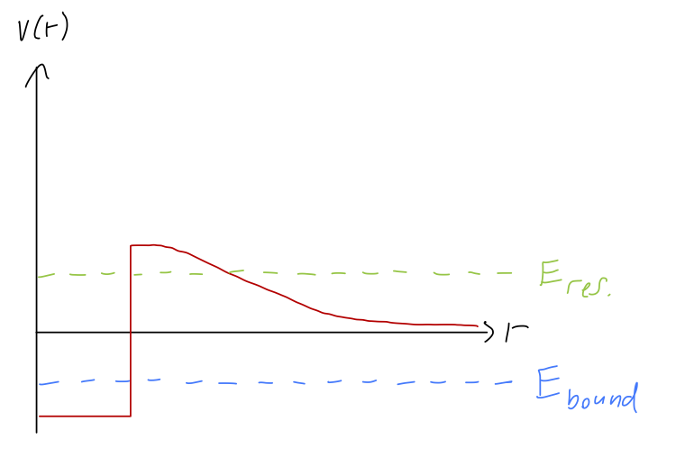
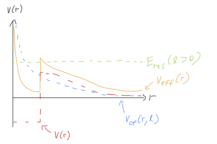
There is one novel feature of this qualitative picture in three dimensions, which is that for l > 0 there is an additional contribution to the effective radial potential, a centrifugal barrier. If we combine this with a potential well, we see that it’s possible for certain energy levels to be purely scattering states for l=0, but become quasi-bound states for larger l. In other words, new resonances can appear at a given energy E for different (larger) values of the angular momentum l:
To get a more quantitative feeling for the behavior of bound states and resonances, let’s first make a useful observation about the S-matrix and the tangent of the phase shift. By definition, \tan \delta_l = \frac{\sin \delta_l}{\cos \delta_l} = -i \frac{e^{2i\delta_l} - 1}{e^{2i\delta_l} + 1} = -i \frac{S_l(k) - 1}{S_l(k) + 1}. If S_l(k) has a pole at some point k^*, then the fraction goes to 1, and we must have \tan \delta_l(k) = -i. Now let’s go back to l=0 and work in terms of our effective range description, k \cot \delta_0 \approx -\frac{1}{a_0} + \frac{1}{2} r_0 k^2. Using what we just showed about the S-matrix, given a pole k=k^\star the left-hand side becomes ik^\star, and we have ik_\star = -\frac{1}{a_0} + \frac{1}{2} r_0 k_\star^2. We can immediately find the solutions: k_\star = \frac{i \pm \sqrt{-1 + 2r_0/a_0}}{r_0} We see that we need both a_0 and r_0 present in order to find a pole solution. If the effective range r_0 is positive and the scattering length a_0 is negative (or vice-versa), then the term under the square root is negative definite, and we find a bound state, k_\star = i\kappa_\star. On the other hand, in any system where a_0 and r_0 have the same sign and 2r_0 / a_0 > 1, we find only resonance solutions, i.e. poles away from the imaginary axis.
One other note of interest is that the limit where k^\star \rightarrow 0 along the imaginary axis corresponds to a_0 \rightarrow \infty. We can see this more directly if we substitute in k^\star = i\kappa_\star to the equation above and rearrange: \frac{1}{a_0} = \kappa_\star - \frac{1}{2} r_0 \kappa_\star^2. In systems where the potential can be tuned, we can adjust \kappa_\star in order to choose the scattering length we want; this can be used practically, for example using magnetic fields to put an atomic gas in a regime favorable for BEC formation as we discussed briefly above. In some cases \kappa_\star can be brought arbitrarily close to zero, resulting in a diverging scattering length a_0 - and therefore a very large cross section! (The physics of what is actually happening here can be deep and interesting, such as the phenomenon of Feshbach resonance; this section of notes is already too long, so I’ll simply link to a review article on the phenomenon for further reading.)
33.6.1 Resonances in the cross section
Let’s expand just a little more on the treatment of a resonance in the S-matrix. Working in terms of energy instead of wave number, a resonance pole occurs at E_\star = E_0 - \frac{i\Gamma_0}{2} (where again we introduce a conventional factor of 2.) If we are doing a real scattering experiment then E > 0 is real and we can never hit the pole. But suppose that we’re very close to the pole in the complex E plane. Then a good approximate description of the S-matrix as a function of energy is given by the pole itself, S(E) \approx \frac{c(E)}{E - E_\star}. To determine the coefficient, we recall that the S-matrix is a phase, which means |S(E)|^2 = 1: 1 = \frac{|c(E)|^2}{|E - E_0 + i\Gamma_0/2|^2} = |c(E)|^2 \frac{1}{(E - E_0 + i\Gamma_0/2)(E - E_0 - i\Gamma_0/2)}. An obvious choice for the normalization is then just the conjugate of the denominator, times a leftover phase: S(E) \approx e^{2i\theta(E)} \frac{E-E_0 - i\Gamma_0/2}{E - E_0 + i\Gamma_0/2} with \theta(E) real. The phase \theta(E) represents additional scattering contributions separate from the pole (the “continuum” contribution), so we’ll set it to zero and focus on just the resonance itself. Adding the expression for S(E) to S^\star(E) and doing some trig identities leads us to the nice result \sin^2 \delta = \frac{\Gamma_0^2}{4(E-E_0)^2 + \Gamma_0^2}. This is for a given scattering channel l, but typically we will only find poles in a single channel at once. If we assume one channel is dominant, then we find the result:
Near a pole in the S-matrix in scattering channel l, the total scattering cross section takes the approximate form
\sigma \approx \sigma_l = \frac{4\pi}{k^2} (2l+1) \sin^2 \delta_l \approx \frac{2\pi \hbar^2}{mE} (2l+1) \frac{\Gamma_0^2}{4(E-E_0)^2 + \Gamma_0^2}.
known as a Breit-Wigner or Lorentzian distribution (up to a factor of 1/E.)
The Breit-Wigner distribution has a characteristic shape, with peak at E_0 and width given by \Gamma_0. In particle physics, unstable particles are not true bound states, but resonances that are probed in scattering experiments. One of the more famous recent examples is the Higgs boson, discovered at the Large Hadron Collider in 2012; one of the ways the Higgs boson can be observed is as a Breit-Wigner resonance in the distribution of pairs of photons.
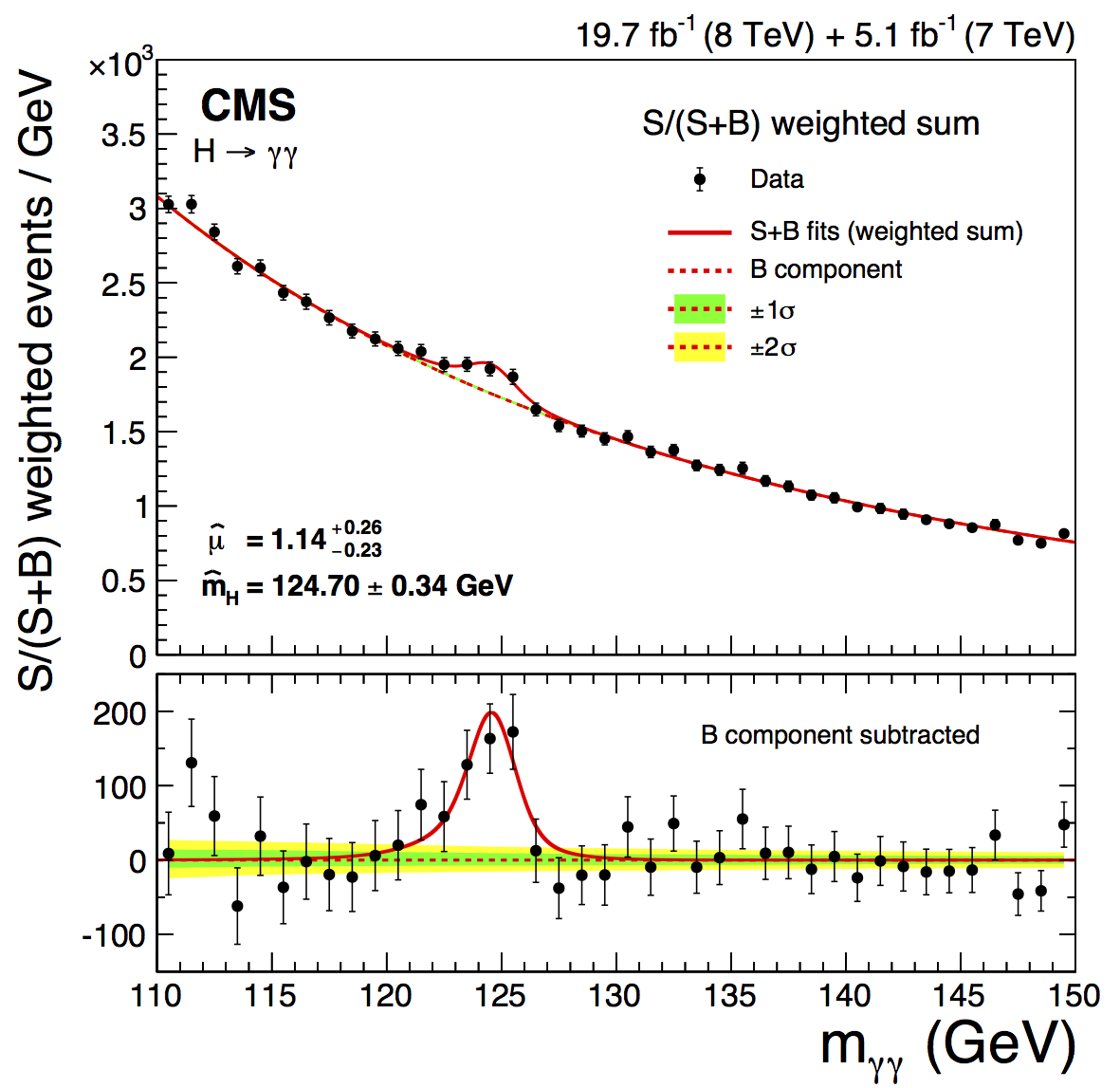 (image credit: CMS experiment.)