16 Density matrix formalism
We’ve now discussed entanglement, which is a key consequence of having a quantum system with more than one particle. However, we’ve also made several informal references by now to the idea of experiments in which we have a single-particle quantum system but we repeat the experiment multiple times - in fact, because of the inherently probabilistic nature of quantum mechanics, having repeated experiments to build up a probability measurement is the only real way to make sense of a quantum system.
Our next goal will be to expand our formalism to deal with this case more rigorously: the presence of a classical ensemble of quantum systems. The same formalism will let us describe classical uncertainty about quantum states (since classical probability is based on the idea of the “population”, which is a theoretical ensemble.)
Let’s start by imagining a situation where we have two sources of uncertainty: in addition to the inherent uncertainty from quantum mechanics, we also have some classical uncertainty about which state we have. We have an experiment which can create either of a pair of quantum states \ket{\chi} or \ket{\psi}, and then measure an observable \hat{O}. However, with each measurement the experiment is set up to randomly select one of the two states, unknown to us, with equal probability p(\chi) = p(\psi) = 0.5.
To separate the two kinds of randomness, we can deal with the quantum uncertainty first and just talk about the average expectation value \left\langle \hat{O} \right\rangle_S = \bra{S} \hat{O} \ket{S} for each state. The rules of classical probability then tell us what we will find for the overall expectation value: \left\langle \hat{O} \right\rangle = \sum_S p(S) \left\langle \hat{O} \right\rangle_S = \frac{1}{2} \left( \left\langle \hat{O} \right\rangle_\chi + \left\langle \hat{O} \right\rangle_\psi \right). We can easily derive a similar formula for the variance of our measurement, \sigma_O^2 = \left\langle \hat{O}^2 \right\rangle - \left\langle \hat{O} \right\rangle^2.
There is another way to set up our quantum system to end up with the same apparent outcome, which is the situation where we have only a single quantum state which is an equal superposition of \ket{\chi} and \ket{\psi}, \ket{\phi} = \frac{1}{\sqrt{2}} (\ket{\chi} + e^{i\alpha} \ket{\psi}), allowing for the presence of an arbitrary phase as part of the superposition which doesn’t affect the relative probabilities. Now if we measure the expectation value in this state, we have the result \left\langle O \right\rangle = \bra{\phi} \hat{O} \ket{\phi} \\ = \frac{1}{2} \left( \bra{\chi} \hat{O} \ket{\chi} + \bra{\psi} \hat{O} \ket{\psi} + e^{i\alpha} \bra{\chi} \hat{O} \ket{\psi} + e^{-i\alpha} \bra{\psi} \hat{O} \ket{\chi} \right) \\ = \frac{1}{2} \left( \left\langle \hat{O} \right\rangle_\chi + \left\langle \hat{O} \right\rangle_{\psi} \right) + {\rm Re} \left[ e^{i\alpha} \bra{\chi} \hat{O} \ket{\psi} \right], using the hermiticity of \hat{O} as an observable to simplify the second term. If the off-diagonal matrix element \bra{\chi} \hat{O} \ket{\psi} = 0, then this is the same prediction as the classical mixture; but even in this case, the two situations are very different. As we’ve seen with the discussion of entanglement, one of the key properties of quantum states is that we will get different outcomes if we measure different observables against the same state. It might be the case that the final term vanishes for some observable \hat{O}, but it will generally not vanish for every possible observable.
This means that as the experimenter, even if the source of our quantum states is a black box, we can almost certainly tell the difference between the classical mixture of states and the quantum superposition of states just by looking at multiple observables and seeing whether the interference effect appears or not.
16.1 Density matrices
We need a better way to distinguish ensembles of quantum states from superposition states. To move towards that, let’s consider the expectation value of an observable in a single state, \left\langle \hat{O} \right\rangle = \bra{\psi} \hat{O} \ket{\psi}. Now we choose a basis \{\ket{n}\} and insert a complete set of states: \left\langle \hat{O} \right\rangle = \sum_{n} \bra{\psi} \hat{O} \ket{n} \left\langle n | \psi \right\rangle \\ = \sum_{n} \left\langle n | \psi \right\rangle \bra{\psi} \hat{O} \ket{n} \\ = {\rm Tr} (\hat{\rho} \hat{O}), where {\rm Tr} denotes the matrix trace, {\rm Tr} {\hat{A}} \equiv \sum_n \bra{n} \hat{A} \ket{n}, and defining the pure density operator or pure density matrix, \hat{\rho} \equiv \ket{\psi} \bra{\psi}. As we have seen in the context of projective measurement, there is a correspondence between a non-degenerate quantum state \ket{a} and the associated projection operator \hat{P}_a = \ket{a}\bra{a}. The density matrix can be thought of as a sort of generalization of this idea: we can take any quantum state \ket{\psi} and replace it with an operator \hat{\rho} that encodes the information of all possible measurement outcomes in that state. (All possible outcomes of measurements, including their probabilities, can be written in the form {\rm Tr} {\hat{\rho} \hat{O}} - for probabilities via Born’s rule, we insert a projection operator \hat{P}_a.)
It is important to keep in mind that there is some information lost when we move from talking about the state vector \ket{\psi} to the pure density matrix \ket{\psi}\bra{\psi}: any overall phase of \ket{\psi} is immediately lost, i.e. the state e^{i\alpha} \ket{\psi} has the same density matrix as \ket{\psi}.
As long as we’re talking about the state of our entire quantum system, the lost phase is a pure global phase and can be safely dropped, as it won’t affect any physical observations. On the other hand, if we try to write density matrices for parts of our system and add them together, we risk getting the wrong answer by dropping an important phase. For example, consider the state \ket{\phi} = \frac{1}{\sqrt{2}} (\ket{\chi} + e^{i\alpha} \ket{\psi}) above. The density matrix for this state is \hat{\rho}_\phi = \ket{\phi} \bra{\phi} \\ = \frac{1}{2} \left( \ket{\chi} \bra{\chi} + \ket{\psi} \bra{\psi} + e^{i\alpha} \ket{\chi} \bra{\psi} + e^{-i\alpha} \ket{\psi} \bra{\chi} \right). This cannot be written as a combination of the individual density matrices \hat{\rho}_\chi and \hat{\rho}_\psi; if we only have those matrices, we have lost the important information about the relative phase \alpha.
The notation of density matrices allows us to very easily extend our description to include ensembles of quantum states, by allowing it to be a mixture of pure density matrices weighted by the classical probability of each state:
Given a random ensemble of normalized quantum states \{ \ket{\psi_i} \} with probabilities p_i, the density matrix describing the system is given by \hat{\rho} \equiv \sum_i p_i \ket{\psi_i} \bra{\psi_i}.
Expectation values of observables over this ensemble are then given by \left\langle \hat{O} \right\rangle = {\rm Tr} ( \hat{\rho} \hat{O}).
The pure density matrix that we introduced above is a special case where there is a single quantum state \ket{\psi} with probability 1. All density matrices satisfy the following conditions, which are straightforward to prove:
- {\rm Tr} (\hat{\rho}) = 1
To prove this, we introduce an orthonormal basis \{\ket{n} \} again, and then write out the trace:
{\rm Tr} (\hat{\rho}) = \sum_n \bra{n} \hat{\rho} \ket{n} \\ = \sum_i \sum_n p_i \left\langle n | \psi_i \right\rangle \left\langle \psi_i | n \right\rangle \\ = \sum_i p_i \left\langle \psi_i | \psi_i \right\rangle. Now as long as the quantum states \ket{\psi_i} are normalized, this is just \sum_i p_i; normalization of the probabilities dictates that \sum_i p_i = 1 (the sum of probabilities for all possible outcomes must be 1), proving the desired result.
- \hat{\rho}^\dagger = \hat{\rho}
This says that \hat{\rho} is Hermitian, and the proof is trivial, following from the fact that (\ket{\psi_i}\bra{\psi_i})^\dagger = \ket{\psi_i} \bra{\psi_i}.
- \bra{\phi} \hat{\rho} \ket{\phi} \geq 0 for any state \ket{\phi} in the Hilbert space
This condition, known as positivity and sometimes just written as \hat{\rho} \geq 0, can be shown similarly to the trace proof above, but now we have a single arbitrary state and no sum. We can still do some simplification: \bra{\phi} \hat{\rho} \ket{\phi} = \sum_i p_i \left\langle \phi | \psi_i \right\rangle \left\langle \psi_i | \phi \right\rangle = \sum_i p_i |\left\langle \phi | \psi_i \right\rangle|^2.
These conditions together guarantee that \hat{\rho} will be a diagonal matrix with eigenvalues between 0 and 1, so they can be interpreted as probabilities.
One of the potentially confusing features of a density matrix is that it can (and often must) be written in terms of a collection of states that are not orthogonal to each other. So although the definition given above bears some resemblance to what we do when we insert a complete set of states, we should not imagine that \ket{\psi_i} have to given any kind of basis. The only condition is that they all have to be normalized states.
In thinking of the density operator as a matrix, we can always write it out in whatever basis we have chosen to work in: \rho_{mn} = \bra{m} \hat{\rho} \ket{n} = \sum_i p_i \left\langle m | \psi_i \right\rangle \left\langle \psi_i | n \right\rangle. Note that in particular, as another way to drive home the point that \ket{\psi_i} don’t form a basis, we can have any number of \ket{\psi_i} mixed together; we could have a 1/20 mixture of 20 different states within a two-state system with d(\mathcal{H}) = 2. The result will be a 2x2 matrix which is a weighted average of 20 2x2 matrices, one for each state in the mixture.
However, even in cases where the number of states in the density matrix is larger than the dimension of our Hilbert space, we are always guaranteed to be able to find a simpler representation. The three properties of density operators proved above guarantee that we can always find a basis of orthonormal eigenstates \{\ket{e_n}\} such that an arbitrary density matrix will take the form \hat{\rho} = \sum_{n=1}^{d(\mathcal{H})} p_n \ket{e_n} \bra{e_n}.
Pure density matrices satisfy one additional property, which is known as idempotence:
- For a pure density matrix only, \hat{\rho}^2 = \hat{\rho}.
The simplest way to prove this is to rely on the fact that we can rewrite an arbitrary density matrix in terms of an orthonormal basis as we just noted, \hat{\rho} = \sum_{n=1}^{d(\mathcal{H})} p_n \ket{e_n} \bra{e_n}. Now we can square this: \hat{\rho}^2 = \sum_{m,n} p_m p_n \ket{e_m} \left\langle e_m | e_n \right\rangle \bra{e_n} \\ = \sum_n p_n^2 \ket{e_n} \bra{e_n}. The only way this can be equal to \hat{\rho} is if p_n^2 = p_n, and the only way that can be true is if each p_n is either equal to 0 or 1. Normalization requires that we can only have a single state in the sum with p_n = 1, and as a result the density matrix becomes an outer product of a single quantum state, which by definition makes it a pure density matrix.
This last property actually suggests a nice and simple way to test whether a given density matrix \hat{\rho} corresponds to a pure state or a mixed state: simply compute the trace {\rm Tr} (\hat{\rho}^2). If the system is in a pure state, then {\rm Tr} (\hat{\rho}^2) = {\rm Tr} (\hat{\rho}) = 1. On the other hand, any mixed state will satisfy {\rm Tr} (\hat{\rho}^2) < 1.
Another way to think of how pure states differ for mixed states is that, if we are handed an arbitrary quantum state \ket{\psi}, we can always do a change of basis for our Hilbert space so that one of the unit vectors points in the direction of \ket{\psi}. In such a basis, the density matrix \ket{\psi} \bra{\psi} becomes extremely simple: \hat{\rho} \rightarrow \left( \begin{array}{cccc} 1 & 0 & 0 & ... \\ 0 & 0 & 0 & ... \\ 0 & 0 & 0 & ... \\ ... & ... & ... & ... \end{array} \right) from which it’s very easy to see the properties described above.
16.2 The Bloch ball
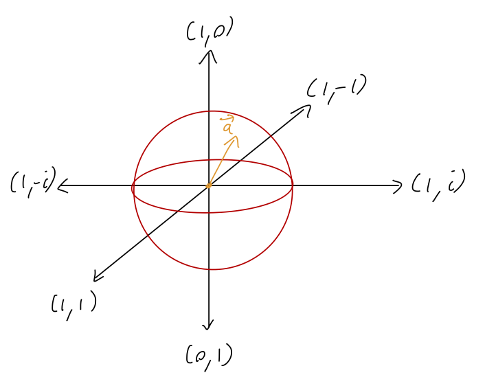
To build some intuition, let’s go back to considering a single two-state system, possibly representing a single silver atom produced in a Stern-Gerlach experiment. As we have seen, we can describe an arbitrary state for such an atom by parameterizing using the Bloch sphere, \ket{\psi} = \cos(\theta/2) \ket{+} + \sin(\theta/2) e^{i \phi} \ket{-}, where \theta, \phi are spherical angles (so these states can be thought of as existing on the surface of a sphere, since there is only a direction and not a magnitude.)
Here, you should complete Tutorial 8 on “Density matrices in the two-state system”. (Tutorials are not included with these lecture notes; if you’re in the class, you will find them on Canvas.)
As we saw in an earlier study of the two-state system, we can write an arbitrary 2x2 matrix as a sum over the identity and the three Pauli matrices, which means that for any density matrix for this system, \hat{\rho}_2 = a_0 \hat{1} + a_x \hat{\sigma}_x + a_y \hat{\sigma}_y + a_z \hat{\sigma}_z. Knowing that this is a density matrix and not just arbitrary imposes some constraints. If we go through the conditions on a density matrix, we find that the most general \hat{\rho}_2 can be written in the simplified form \hat{\rho}_2 = \frac{1}{2} \left( \hat{1} + \vec{a} \cdot \hat{\vec{\sigma}} \right), where the vector of parameters \vec{a} is real and satisfies the condition |\vec{a}| \leq 1.
Confirm that applying the three conditions 1-3 given above that a density matrix must satisfy leads to the parameterization shown above with |\vec{a}| \leq 1.
Answer:
First of all, Hermiticity \hat{\rho}_2^\dagger = \hat{\rho}_2 tells us that the four a_i coefficients are all real. Second, all of the Pauli matrices have zero trace, so the trace of this matrix is simply 2 a_0; unit trace therefore implies that we can eliminate a_0 and rewrite in the conventional form \hat{\rho}_2 = \frac{1}{2} \left( \hat{1} + \vec{a} \cdot \hat{\vec{\sigma}} \right), combining the remaining coefficients into a vector \vec{a}. Third, we have the positivity condition \hat{\rho}_2 > 0. This one is a bit more subtle, but it will hold as long as all of the eigenvalues of \hat{\rho}_2 are positive. The two eigenvalues satisfy the relations {\rm Tr} (\hat{\rho}_2) = \lambda_1 + \lambda_2 \\ \det(\hat{\rho}_2) = \lambda_1 \lambda_2 We already know the trace, now we need the determinant: \det(\hat{\rho}_2) = \frac{1}{4} \left| \begin{array}{cc} 1 + a_z & a_x - ia_y \\ a_x + ia_y & 1 - a_z \end{array} \right| \\ = \frac{1}{4} (1 - a_z^2 - a_x^2 - a_y^2) \\ = \frac{1}{4} (1 - |\vec{a}|^2). Between the two conditions, we see that |\vec{a}| \leq 1 will give a valid density matrix.
If we have a pure state specifically, then the density matrix will satisfy {\rm Tr} (\hat{\rho_2}^2) = 1. Plugging in the parameterization above, {\rm Tr} (\hat{\rho_2}^2) = \frac{1}{4} {\rm Tr} (\hat{1} + 2(\vec{a} \cdot \hat{\vec{\sigma}}) + |\vec{a}|^2 \hat{1}) \\ = \frac{1}{2} (1 + |\vec{a}|^2) using (\vec{a} \cdot \vec{\hat{\sigma}})^2 = \sum_{i,j} a_i a_j \hat{\sigma}_i \hat{\sigma}_j = \sum_i a_i^2 \hat{1} to simplify the fourth term. For this to be 1, then, we need |\vec{a}| = 1.
Putting all of this together, we have a nice and geometric picture: for a two-state system, all possible density matrices are described by the choice of a vector \vec{a} with length |\vec{a}| \leq 1, which describes a sphere with radius 1. If |\vec{a}| = 1, then we are on the surface of the sphere, and these are the pure states; in fact, this recovers the Bloch sphere parameterization we already had, based on the direction in which \vec{a} points. However, we’ve now added the interior of the sphere by allowing |\vec{a}| < 1, which describes all of the possible mixed states. This parameterization defines the Bloch ball (sometimes confusingly also called the “Bloch sphere”, but in more formal mathematics a “sphere” is the surface while a “ball” includes the interior.)
Let’s do a couple of quick examples of mapping between states and density matrices in the two-state system. First, the pure state \ket{\uparrow}: \hat{\rho} = \ket{\uparrow} \bra{\uparrow} = \left( \begin{array}{cc} 1 & 0 \\ 0 & 0 \end{array} \right). In terms of our Pauli matrix basis, this is \tfrac{1}{2} (\hat{1} + \hat{\sigma}_z), which tells us that \vec{a} = (0,0,1) - with length 1 as expected for a pure state, and pointing in the +z direction.
Next, let’s try the mixed state which is 50% \ket{\uparrow} and 50% \ket{\downarrow}: \hat{\rho} = \frac{1}{2} \ket{\uparrow} \bra{\uparrow} + \frac{1}{2} \ket{\downarrow} \bra{\downarrow} \\ = \frac{1}{2} \left(\begin{array}{cc} 1 & 0 \\ 0 & 1 \end{array} \right) = \frac{1}{2} \hat{1}. For this state we see that we simply have \vec{a} = 0.
As we have noted above, in general we can’t go backwards from density matrix to the corresponding mixture of states, since some phase information is lost in the density matrix. This means that the preparation of a given density matrix (i.e. what mixture of states is used to create it) is usually ambiguous. For the example here, a 50-50 mixture of \frac{1}{\sqrt{2}} (\ket{\uparrow} \pm \ket{\downarrow}) - the spin eigenstates in the x direction instead of the z direction - will give exactly the same density matrix with \vec{a} = 0.
The vector \vec{a} has a simple physical meaning: we can interpret it as a polarization vector. If we imagine using the density matrix to describe the source for a Stern-Gerlach experiment, the polarization of the source describes the quantum state of the incoming silver atoms. If we just take the raw input of silver atoms from a furnace, they will in general be unpolarized, meaning an even mixture of spins in any direction; the corresponding density matrix is given by \vec{a} = 0. If we take the output from a single Stern-Gerlach analyzer, we know the spin state in the corresponding direction with 100% certainty, so this will be a pure state, polarized in the associated direction.
Finally, I’ll comment in passing that this may seem very different from the use of a polarization vector for light, but in fact they are the same thing; we haven’t talked much about light as a quantum system, but light has two orthogonal polarization states (say in the x and y direction), which is a perfect candidate for a two-state system description. In such a setup, all pure states represent polarized light in a particular direction, while the mixed state with \vec{a} = 0 represents unpolarized light.
16.3 Quantum statistical mechanics
Another very common use of density matrices to represent a mixture of states occurs in statistical mechanics, to describe a quantum system at finite temperature. All of stat mech is built on the idea of constructing ensembles of microstates, so the density matrix is a natural way to proceed.
There is an argument that tries to derive the form of a stat-mech density matrix shown in Sakurai, but it’s simpler just to start with the idea that we want to construct a canonical ensemble, which is a distribution of states distributed according to e^{-\beta E}, with \beta \equiv 1 / (k_B T), where k_B is the Boltzmann constant and T is the temperature. This is simple to express as a density matrix: \hat{\rho}(T) = \frac{1}{Z} \sum_i e^{-\beta E_i} \ket{E_i} \bra{E_i} where \ket{E_i} are the energy eigenstates, and Z is the partition function, Z = \sum_i e^{-\beta E_i}. Now, we can recognize \sum_i E_i \ket{E_i} \bra{E_i} as just the Hamiltonian, \hat{H}, written in its own eigenbasis. This means that we can write the canonical-ensemble density matrix \hat{\rho}(T) as simply \hat{\rho}(T) = \frac{1}{Z} e^{-\beta \hat{H}} and Z = {\rm Tr} (e^{-\beta \hat{H}}). Note that from this version it’s obvious to see by construction that [\hat{\rho}(T), \hat{H}] = 0
We won’t go much further into statistical mechanics at this point, but we have enough at this point to do a simple example that everyone should see, which is a spin-1/2 system in a magnetic field at finite temperature. We return to the simple Hamiltonian we’ve studied before with an applied magnetic field in the z direction, \hat{H} = \frac{\hbar \omega}{2} \hat{\sigma}_z with \omega \equiv egB/(2mc). Working in the spin-z eigenbasis, \hat{\sigma}_z is diagonal which means it’s trivial to write out the density matrix by exponentiating: \hat{\rho}(T) = \frac{1}{Z}e^{-\beta \hat{H}} = \frac{1}{Z} \left( \begin{array}{cc} e^{-\beta \hbar \omega/2} & 0 \\ 0 & e^{+\beta \hbar \omega/2} \end{array} \right) and the partition function is Z = {\rm Tr} (e^{-\beta H}) = 2 \cosh \left( \frac{\beta \hbar \omega}{2} \right). First of all, using what we know about the density matrix, let’s evaluate how mixed this state is: we have {\rm Tr} (\hat{\rho}(T)^2) = \frac{1}{Z^2} \left( e^{-\beta \hbar \omega} + e^{+\beta \hbar \omega}\right) \\ = \frac{\cosh (\beta \hbar \omega)}{2 \cosh^2 (\beta \hbar \omega/2)} \\ = 1 - \frac{1}{2 \cosh^2(\beta \hbar \omega/2)} using a double-angle identity. To recover a pure state, this only goes to 1 in the limit that \cosh(\beta \hbar \omega/2) \rightarrow \infty, which means either \omega is very large (strong magnetic field) or \beta is very large (low temperature.) Physically, either of these two cases leads to the spin sitting in a pure state which is the lower-energy state aligned with the magnetic field direction.
Finally, let’s get a little bit of physics out since we have the density matrix and the partition function. We can calculate the magnetization, which is the expectation value of the magnetic moment of our spin: \vec{M} = \left\langle \hat{\vec{\mu}} \right\rangle = \left\langle \frac{eg}{mc} \hat{\vec{S}} \right\rangle. It’s easy to verify (or argue from symmetry) that only the z component will be non-zero, and we can calculate that from our density matrix: M_z = \frac{eg\hbar}{2mc} \left\langle \hat{\sigma}_z \right\rangle = \frac{eg\hbar}{2mc} {\rm Tr} (\hat{\rho}(T) \hat{\sigma}_z) \\ = \frac{eg\hbar}{2mc} \frac{1}{2 \cosh(\beta \hbar \omega/2)} (e^{-\beta \hbar \omega/2} - e^{+\beta \hbar \omega/2}) \\ = -\frac{eg\hbar}{2mc} \tanh \left( \frac{\beta \hbar \omega}{2} \right). If we switch off the magnetic field, then \omega = 0 and we find that M_z = 0; this is what we expect, since this is a description of an ensemble of spins at a finite temperature, for which the spins will have random orientation so the total magnetization will average to zero. Similarly in the limit \beta = 0 (infinite temperature) the magnetic field becomes irrelevant and the magnetization goes away.
More generally, this is an induced magnetization, since it’s only non-zero with an applied magnetic field, making this a paramagnetic system. For small |B|, we can characterize this in terms of Curie’s law, |\vec{M}| = \chi |B|, which we can see does hold here since the \tanh above is linear in \vec{B}. Plugging in, we find for the susceptibility \chi = \frac{eg \hbar}{2mc} \frac{\beta \hbar \omega}{2} \frac{1}{|B|} \\ = \left( \frac{eg}{2mc} \right)^2 \frac{\hbar^2}{2 k_B T}.
Coming back to physics once more, we see that larger charge, lighter mass, or lower temperature all increase the susceptibility, all of which make sense (they give a larger magnetic moment, or for the temperature, a less randomized magnetic moment.)
16.4 Entanglement and density matrices
Now that we have the formalism down, we can return to our study of entanglement and find another very useful application of density matrices. Let’s return to our experimenters Alice and Bob who are sharing entangled EPR pairs, \ket{\psi_{EPR}} = \frac{1}{\sqrt{2}} (\ket{\uparrow}_A \ket{\downarrow}_B - \ket{\downarrow}_A \ket{\uparrow}_B). As before we describe the full quantum system for a single EPR pair using a four-dimensional Hilbert space \mathcal{H}_A \otimes \mathcal{H}_B spanned by direct products \{\ket{\uparrow}_A \ket{\uparrow}_A, \ket{\uparrow}_A \ket{\downarrow}_B, \ket{\downarrow}_A \ket{\uparrow}_B, \ket{\downarrow}_A \ket{\downarrow}_B\}, which means an arbitrary state will have a four-by-four density matrix. It’s straightforward to calculate the full density matrix for the EPR state: \hat{\rho}_{EPR} = \frac{1}{2} \left( \begin{array}{cccc} 0 & 0 & 0 & 0 \\ 0 & 1 & -1 & 0 \\ 0 & -1 & 1 & 0 \\ 0 & 0 & 0 & 0 \end{array} \right). (You can easily check that {\rm Tr} (\hat{\rho}_{EPR}) = {\rm Tr} (\hat{\rho}_{EPR}^2) = 1 as expected for a pure density matrix.) This is a perfectly good density matrix but only to describe the combined system where both spins are in the same laboratory. There are more interesting consequences to thinking about the system in the situation described for the EPR paradox, where Alice and Bob are working in labs separated by a large distance.
Using the combined density matrix, we can compute the outcomes of measurements from traces over the appropriate operators. But now let’s think about the separated case, where Alice only has access to her own spin. This means in mathematical terms that any possible operator she can measure takes the form of something which is the identity with respect to Bob’s spin: \hat{O}_A = \hat{A} \otimes \hat{1}. What does this imply for her measurements? To work this out, we need to get a little bit more abstract first.
16.4.1 Partial traces
Let’s define some more general statements regarding quantum systems of the form \mathcal{H}_A \otimes \mathcal{H}_B (known as a “bipartite system”.) We take \{ \ket{a_m} \} and \{ \ket{b_\mu} \} to be the basis kets for \mathcal{H}_A and \mathcal{H}_B respectively. We can take any arbitrary quantum state \ket{\psi} and expand it in the joint basis formed by direct product, \ket{\psi} = \sum_{m=1}^{d(\mathcal{H}_A)} \sum_{\mu=1}^{d(\mathcal{H}_B)} c_{m\mu} \ket{a_m} \otimes \ket{b_\mu}. For operators, let’s consider the trace, in this basis given by the formula {\rm Tr} (\hat{O}) = \sum_{m,\mu} (\bra{a_m} \otimes \bra{b_\mu}) \hat{O} (\ket{a_m} \otimes \ket{b_\mu}). If the operator \hat{O} happens to break apart into a direct product itself, then we can use this to find further simplifications - for example, it’s easy to show that the trace over such an operator breaks into {\rm Tr} (\hat{A} \otimes \hat{B}) = {\rm Tr} (\hat{A}) {\rm Tr} (\hat{B}), where all traces are taken with respect to the appropriate Hilbert space (so over \mathcal{H}_A, \mathcal{H}_B for \hat{A} and \hat{B} respectively.)
Although most operators won’t break apart into direct products like this, it’s still useful to think about summing over just part of the basis. We define the partial trace as a trace with respect to one Hilbert space or the other, instead of both: {\rm Tr} _B(\hat{O}) \equiv \sum_{k,m} \sum_\mu \ket{a_k} (\bra{a_k} \otimes \bra{b_\mu}) \hat{O} (\ket{a_m} \otimes \ket{b_\mu}) \bra{a_m}, and {\rm Tr} _A(\hat{O}) is defined similarly. A complete trace gives us a number as a result, but since this is a partial trace, the result is still an operator. But this operator lives in the Hilbert space \mathcal{H}_A, instead of the combined \mathcal{H}. Going back to the simpler case where the operator is a direct product, it’s again easy to show that {\rm Tr} _B(\hat{A} \otimes \hat{B}) = \hat{A} and {\rm Tr} _A(\hat{A} \otimes \hat{B}) = \hat{B}.
Now let’s look at what these partial traces imply for a density matrix; let’s just study the pure density matrix \hat{\rho} = \ket{\psi}\bra{\psi}, everything we find will generalize simply. We can expand this density matrix in our joint basis as \hat{\rho} = \sum_{m,\mu} \sum_{n,\nu} c_{m\mu} c_{n\nu}^\star \ket{a_m} \otimes \ket{b_\mu} \bra{a_n} \otimes \bra{b_\nu}. The full trace of this matrix gives 1 by definition, but what do we get if we do a partial trace? Let’s try it: {\rm Tr} _B(\hat{\rho}) = \sum_{i,j} \sum_\kappa \ket{a_i}\bra{a_j} (\bra{a_i} \otimes \bra{b_\kappa}) \hat{\rho} (\ket{a_j} \otimes \ket{b_\kappa}) \\ = \sum_{i,j} \sum_\kappa c_{i\kappa} c_{j\kappa}^\star \ket{a_i} \bra{a_j}. If we take a final trace over this, we get {\rm Tr} ({\rm Tr} _B(\hat{\rho})) = \sum_{n} \bra{a_n} {\rm Tr} _B(\hat{\rho}) \ket{a_n} = \sum_{n,\kappa} |c_{n\kappa}|^2 = |\psi|^2 = 1. So the trace is still 1, and in fact, this partially-traced object still has all of the correct properties to be a density matrix itself. We define this to be the reduced density matrix, and we can get one for each smaller Hilbert space by tracing over the other one: \hat{\rho}_A \equiv {\rm Tr} _B(\hat{\rho}), \\ \hat{\rho}_B \equiv {\rm Tr} _A(\hat{\rho}).
Now, just because these are valid density matrices, that doesn’t tell us what information on the physics of our system they actually contain. In fact, it’s straightforward to see that the partial trace loses some information from the original density matrix \hat{\rho}, so that for an arbitrary operator \hat{O} on the product Hilbert space, we don’t have enough information in the reduced density matrices to compute \left\langle \hat{O} \right\rangle.
However, consider the special operator \hat{A} \otimes \hat{1}. If we do out the math, we find the result \left\langle \hat{A} \otimes \hat{1} \right\rangle = {\rm Tr} (\hat{\rho}_A \hat{A}), and of course we would find a simliar result for \left\langle \hat{1} \otimes \hat{B} \right\rangle using the other reduced density matrix.
Expand out and show the result for the expectation value above.
Answer:
Let’s go through it: \left\langle \hat{A} \otimes \hat{1} \right\rangle = \bra{\psi} (\hat{A} \otimes \hat{1}) \ket{\psi} \\ = \sum_{m,\mu} \sum_{n,\nu} c_{m\mu} c_{n\nu}^\star (\bra{a_n} \otimes \bra{b_\nu}) (\hat{A} \otimes \hat{1}) (\ket{a_m} \otimes \ket{b_\mu}) \\ = \sum_{m,n} \sum_{\mu,\nu} c_{m\mu} c_{n\nu}^\star \bra{a_n} \hat{A} \ket{a_m} \left\langle b_\nu | b_\mu \right\rangle \\ = \sum_{m,n} \sum_\mu c_{m\mu} c_{n\mu}^\star \bra{a_n} \hat{A} \ket{a_m} \\ = \sum_{m,n} \sum_\mu \sum_k c_{m\mu} c_{n\mu}^\star \bra{a_n} \hat{A} \ket{a_k} \left\langle a_k | a_m \right\rangle \\ = \sum_k \sum_{n} \sum_\mu \bra{a_k} \left[ c_{k\mu} c_{n \mu}^\star \ket{a_k}\bra{a_n} \hat{A} \right] \ket{a_k} \\ = \sum_k ({\rm Tr} _B(\hat{\rho})_{kn} \hat{A}_{nk}) \\ = {\rm Tr} ( \hat{\rho}_A \hat{A}).
16.4.2 Reduced density matrices and entanglement
Now we have the math in hand to go back and understand the physics. When Alice makes a measurement solely of spin A, her measurements take exactly the form \hat{A} \otimes \hat{1}, which means that the outcome of any measurement Alice does can be expressed using the reduced density matrix \hat{\rho}_A, which involves computing the partial trace {\rm Tr} _B(\hat{\rho}) over the original, full density matrix. This is sometimes referred to as “tracing out” the spin B degree of freedom. It makes perfect physical sense that this is how things work: Alice only has access to her own spin A, so anything she does is from a state of maximum ignorance about what Bob’s spin is doing, hence her predictions involve summing over all possibilities for spin B. The “local density matrix” that describes Alice’s system in isolate is precisely the reduced density matrix \hat{\rho}_A.
Let’s calculate the reduced density matrix and inspect it: \hat{\rho}_A = {\rm Tr} _B (\hat{\rho}) = \ket{a_i} \bra{a_j} \left[ (\bra{a_i} \otimes \bra{\uparrow}_B) \hat{\rho} (\ket{a_j} \otimes \ket{\uparrow}_B) + (\bra{a_i} \otimes \bra{\downarrow}_B) \hat{\rho} (\ket{a_j} \otimes \ket{\downarrow}_B) \right], where \ket{a_i} is standing in for the two states \ket{\uparrow}_A, \ket{\downarrow}_A, and the result will be a 2x2 matrix (as it should be to describe just Alice’s two-state spin system.) We can just write out all of these matrix elements by hand, but since we already have \hat{\rho} written out in matrix form, we can also see how to evaluate the trace based on that. For example, the \bra{\uparrow} \hat{\rho}_A \ket{\uparrow} element of the reduced matrix element is given by adding together \hat{\rho}_{(\uparrow \uparrow, \uparrow \uparrow)} + \hat{\rho}_{\uparrow \downarrow, \uparrow \downarrow}, which (in the way we’ve written the basis) is just a trace taken over the upper left block:
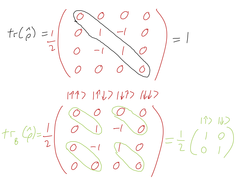
We see that the result is \hat{\rho}_A = \frac{1}{2} \left( \begin{array}{cc} 1 & 0 \\ 0 & 1 \end{array} \right). This is a mixed density matrix, not pure! If we calculate {\rm Tr} (\hat{\rho}_A^2), we find that it is equal to 1/2. In fact, this is what we should expect, because we already know from our EPR discussion that in isolation, Alice is free to measure along any axis at all and will always find the same outcome of 50% odds of either spin-up or spin-down along that axis, meaning this is an unpolarized spin state (and if you go back to the Bloch ball parameterization, you will see that this is precisely the density matrix at the center of the ball with \vec{a} = 0.)
In fact, it is not a coincidence that we found a mixed density matrix: it is a direct consequence of the fact that the EPR state we started with to write the full 4x4 density matrix is entangled. Given a pure-state density matrix over a bipartite system, if the partial-trace density matrix is mixed, then the pure state is entangled. Intuitively, if the initial state is not entangled (and thus takes the form \ket{\psi} = \ket{a} \otimes \ket{b}), then tracing out Hilbert space B still leaves us with a pure state \ket{a} on Hilbert space A (or vice-versa.)
This intuitive statement isn’t a rigorous proof; to put things on firmer ground, it’s helpful to start with the concept of Schmidt decomposition. Suppose as above that we have an arbitrary pure state decomposed over our bipartite Hilbert space given some choice of basis, \ket{\psi} = \sum_{m=1}^{d(\mathcal{H}_A)} \sum_{\mu=1}^{d(\mathcal{H}_B)} c_{m\mu} \ket{a_m} \otimes \ket{b_\mu}. Although this is a state vector with respect to \mathcal{H}, since it’s written over a direct-product basis, the coefficients c_{m\mu} also form a matrix. This means that we can attempt to diagonalize it by changing our basis - but in general, c_{m\mu} is usually a rectangular and not a square matrix, which means it admits different methods than we’re used to.
The method of choice for this case is known as a singular value decomposition, or SVD. This is a diagonalization of an arbitrary rectangular matrix M using a transformation of the form U M V^{\dagger}, where U and V are different unitary matrices (of different sizes); this is to be compared with M \rightarrow U M U^{\dagger} for diagonalizing a square matrix. In this particular case, the SVD looks exactly like c \rightarrow U_a c U_b^{\dagger} where U_a, U_b are unitary matrices that give a change of basis on the separate \mathcal{H}_A and \mathcal{H}_B spaces. I won’t go through any proofs here, but given a pure state, applying an SVD yields a diagonal and positive result for \ket{\psi} in a specific basis.
Given a pure state \ket{\psi} that exists on a bipartite Hilbert space \mathcal{H} = \mathcal{H}_A \otimes \mathcal{H}_B with d(\mathcal{H}_A) \leq d(\mathcal{H}_B), there is a choice of basis for both subspaces for which the state vector takes the form
\ket{\psi} = \sum_{i=1}^{d(\mathcal{H}_A)} \sqrt{p_i} \ket{a_i} \otimes \ket{\tilde{b}_i}, where the orthonormal vectors \ket{\tilde{b}_i} are obtained from a full basis \ket{b_\mu} for \mathcal{H}_B by the transformation \ket{\tilde{b}_i} \equiv \sum_\mu U_{i\mu} \ket{b_\mu}.
The coefficients \sqrt{p_i} are square roots of probabilities that occur when taking partial traces of this pure state. In particular, \hat{\rho}_A = {\rm Tr} _B(\ket{\psi} \bra{\psi}) = \sum_i p_i \ket{a_i} \bra{a_i}, \\ \hat{\rho}_B = {\rm Tr} _A(\ket{\psi} \bra{\psi}) = \sum_i p_i \ket{\tilde{b}_i} \bra{\tilde{b}_i}.
This is specifically a form of singular value decomposition known as “compact SVD”, where we do some projection in addition to the basis change on the larger Hilbert space \mathcal{H}_B in order to end up with a square matrix. The values \sqrt{p_i} are known as the singular values of the matrix c_{m\mu} that we started with; they’re generalizations of eigenvalues. They also correspond to exactly the probabilities for the mixed-state density matrices we get when we compute a partial trace over either subspace.
Schmidt decomposition can be useful for a variety of things, but the key observation we can make from it now is that the only way for \hat{\rho}_A and \hat{\rho}_B to be pure density matrices is if there is a single p_k = 1 and all other p_i = 0. If this is true, then the original state is simply \ket{\psi} = \ket{a_k} \otimes \ket{\tilde{b}_k}, which is a product state and thus not entangled. Going the other direction, if \ket{\psi} is an entangled state, then there is no change of basis which allows us to choose a single p_k = 1; it must be a linear combination of at least two direct-product basis states. So we have a direct test for entanglement:
A state \ket{\psi} in bipartite Hilbert space \mathcal{H} = \mathcal{H}_A \otimes \mathcal{H}_B is entangled if:
- It cannot be written as a direct product \ket{\phi_A} \otimes \ket{\chi_B};
- Either of the reduced density matrices \hat{\rho}_A, \hat{\rho}_B is a mixed density matrix;
- The number of non-zero singular values \sqrt{p_i} of \ket{\psi} (known as the Schmidt number) is greater than one.
Each of these conditions implies the other two.
There is a corollary to the statement that pure states will usually give us mixed states when we partial trace, which is that we can also go the other way: any mixed density matrix can be written as a partial trace over a pure state in a larger Hilbert space. Constructing such a pure state is known as purification. This should be mostly regarded as a mathematical trick (since in the general case it requires us to invent a new and larger Hilbert space,) but it is useful to know about.
Finally, these results have important implications for how we think about realistic quantum systems. For any isolated quantum system S we want to study in experiment, there will generally be some coupling to the surrounding environment E. In other words, even if we want to just study a pure quantum system, in practice we are always working with the larger Hilbert space \mathcal{H} = \mathcal{H}_S + \mathcal{H}_E. This means that our system is really described by a partial trace over the environment surrounding it, which in the presence of any entanglement with the environment will leave us with a mixed state where we probably wanted a pure state! The effect of the environment, if we’re not careful, is to add classical noise that overwhelms the delicate quantum information that we want to work with.