Appendix B — Invitation to quantum field theory
One piece of physics that we haven’t studied in these notes is the Dirac equation, which allows a relativistic treatment of the motion of an electron, or any other spin-1/2 particle. However, even the Dirac equation turns out to be a small part of the complete story. Truly including relativity with quantum mechanics requires the use of quantum field theory. The key word here is “field”. A field F is a physical object which takes on some value everywhere in space and time, i.e. F = F(\mathbf{x},t). This is as opposed to a particle, which (classically) has a definite position in space.
Of course, we know that in quantum mechanics, our particles no longer have definite positions, but rather have wave-like properties of their own, described by the wavefunction \psi(x,t) which gives the probability density for that particle’s location. Technically the wavefunction itself is a field, but don’t get confused - it’s still describing the physics of a single point-like particle. What we don’t know how to do is quantize something like a vibrating string which is already described by a field. (Or, more importantly, we might ask: how do we quantize the electromagnetic field? We have dealt with such fields in quantum mechanics, but only as classical backgrounds; quantization of light requires quantum field theory.)
Borrowing a diagram from Sidney Coleman, we can think of two procedures, quantization and the continuum limit. Quantum field theory is what results from combining both procedures:
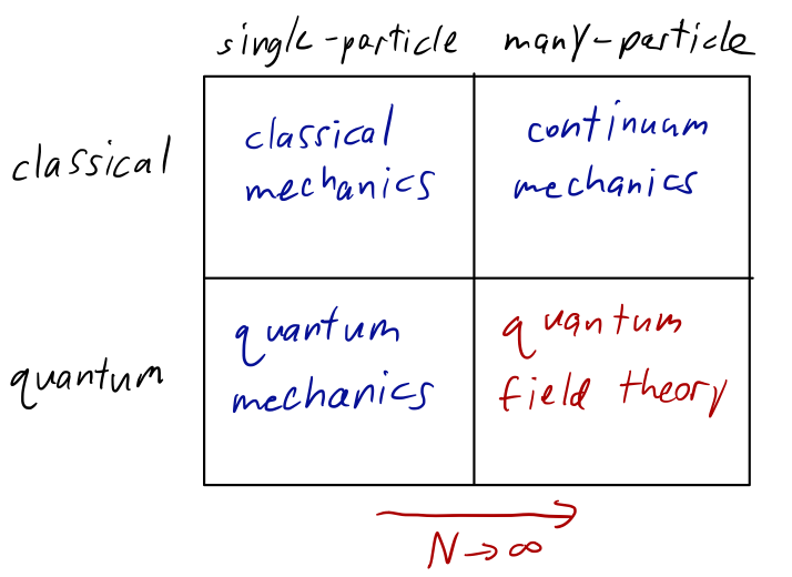
It should be pointed out that we don’t have to use a continuous theory to study, say, a condensed matter system. Often, such systems aren’t even continuous, but exist on a real and finite lattice: we can describe all of their physics in principle just using the Schrodinger equation. But this quickly becomes completely intractable for any realistic system, where there can be 10^{24} particles or more to work with. A continuous description is very powerful for understanding the collective properties of such a system, particularly in the context of phase transitions and critical phenomena.
But wait: I started this discussion by talking about the Dirac equation. We can draw a similar diagram for another limit we already understand for classical systems, the relativistic limit - what is the appropriate extension of quantum mechanics there?
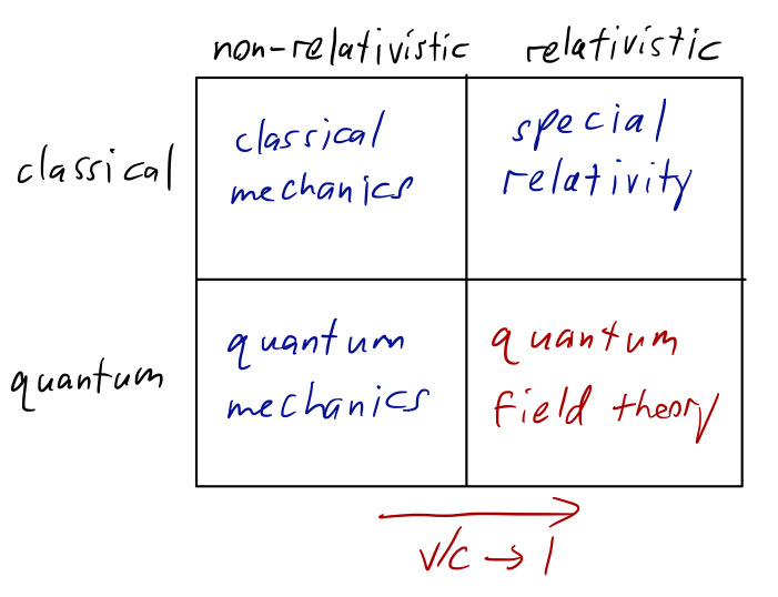
At the intersection of quantum mechanics and special relativity, we find quantum field theory again! This should come as a surprise - it’s not obvious that this should be true. Why should we need continuous fields to understand the relativistic behavior of a single particle?
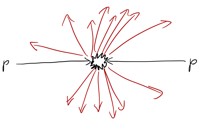
The simplest answer is that it is true: there were many attempts to simply promote single-particle descriptions such as the Schrodinger equation to relativistic equations, and they failed spectacularly, giving states with negative energy and violation of the laws of probability. But there are two other explanations which can give us a bit more physical insight. First, relativity implies matter-energy equivalence with the equation E=mc^2. Suppose we trap a particle and localize its position to within some uncertainty \Delta x. The uncertainty principle tells us that \Delta p \Delta x\geq \hbar, or \Delta E \Delta x \geq \hbar c. using E \approx pc for large enough momentum. If this uncertainty is sufficiently large, then there is potentially enough energy in the system to pop new particles out of the vacuum: in other words, we are now uncertain about even how many particles are in our trap. The threshold for this is \Delta E \gtrsim mc^2, or \Delta x = \lambda_C \sim \frac{\hbar}{mc}. This length scale is known as the Compton wavelength of a particle, and we can think of it as the length scale at which a non-relativistic, single-particle description of the system has to break down. We can observe this experimentally: for example, at the Large Hadron Collider, collisions of two protons frequently produce many different final-state particles.
So, we arrive at the key insight: matter-energy equivalence in relativity requires us to be able to create and destroy particles, which necessarily forces us to describe our theory using fields instead of single particles, hence quantum field theory.
Strictly speaking, creation of particles from the vacuum can’t happen completely arbitrarily. The electron, for example, is stable and can’t be created from, or decay into, the vacuum state. On more general grounds, just creating a single electron out of nothing would violate charge conservation. But if there is an antiparticle with exactly opposite properties to the electron, then we can always create a particle-antiparticle pair from energy, and no symmetries are violated. (And indeed there is - the positron!)
B.0.1 Propagators and causality
The existence of antiparticles is an experimental fact, but it also gives us one more motivation for why quantum field theory is needed to combine relativity and quantum mechanics. Let’s consider the probability amplitude for a quantum mechanical particle to propagate from the origin to another point \mathbf{x}, given by the propagator: K(x', t; x, t_0) = \bra{\vec{x}'} e^{-i\hat{H} (t-t_0)/\hbar} \ket{\vec{x}} Consider a completely free particle, so its Hamiltonian is just the kinetic energy \hat{H} = \hat{\vec{p}}^2 / 2m. We calculate this for the one-dimensional case before, which is good enough to see the effect we’re looking for. Placing the initial point at the origin (0,0) and dropping the primes, we have K(x, t; 0, 0) = \sqrt{\frac{m}{2\pi i \hbar t}} e^{imx^2 / (2\hbar t)}. The problem with this expression is that it is non-zero for any finite t and any x. This implies that if, say, we fix x and take t \rightarrow 0, eventually we predict a non-zero probability for propagation faster than the speed of light. Thus, our amplitude formula leads to violation of causality!
You might expect that the culprit here is the use of the non-relativistic energy, and we could fix things by using E = c\sqrt{p^2 + m^2c^2} instead. If we do this and then insert a complete set of momentum states to evaluate, we have K_{\rm rel}(x, t; 0, 0) = \int_{-\infty}^\infty \frac{dp}{2\pi \hbar} e^{-ict\sqrt{p^2 + m^2 c^2}} e^{ipx/\hbar} This is not a Gaussian integral, but we can use the method of stationary phase to find that asymptotically, for x^2 \gg (ct)^2 (i.e. far outside the light cone), we have K_{\rm rel}(x,t; 0, 0) \sim e^{-mc|x|/\hbar}. This is at least an improvement, because we have exponential suppression outside of the light cone instead of just oscillatory behavior; but it still implies propagation faster than light, which leads to violations of casuality in special relativity (and is inconsistent with experiment!)
In full quantum field theory, there are two parts to the resolution of this question. The first is that once we allow quantum fields, the propagator doesn’t really mean the same thing anymore; the particles at both 0 and x are both excitations of the same field, but they could be separate single-particle excitations - we can’t really “track” the particle from initial to final point. If this was a QFT class, we would work to define a modified version of the propagator to ask the more precise question: does the order of measurements matter between two spacelike-separated points?
And the answer will turn out to be no, but only because we will find two terms that individually are only exponentially suppressed, but that will cancel exactly. The two terms are exactly related to propagation of particles, and propagation of antiparticles - both are required. So in quantum field theory, the existence of antiparticles is required for compatibility with special relativity and causality!