29 Time-dependence: sudden and adiabatic approximations
All of the approximation methods we’ve studied so far are static; they are methods for finding energy eigenvalues and eigenstates. While this can be used to get some information about time dependence, there is a lot to gain by considering more explicit methods for approximation that build in time evolution as well. We also, as of yet, have very few tools to handle the situation where the Hamiltonian itself has explicit time dependence.
We’ll begin with the sudden and adiabatic approximations, in which the nature of the time-dependence itself (very fast or very slow) allows us to make useful approximations. Then we’ll turn to a more general discussion of time-dependent perturbation theory.
29.1 Sudden approximation
We begin with the simpler approximation, which is the sudden approximation. The idea is simply that there is a sudden change to our Hamiltonian, which means that at some time t_S, the Hamiltonian suddenly changes from one form to another. Labelling the initial Hamiltonian as \hat{H}_0 and the new Hamiltonian as \hat{H}_1, then, \hat{H} = \begin{cases} \hat{H}_0,& t < t_S; \\ \hat{H}_1,& t \geq t_S. \end{cases}
This approximation is the simplest version of time dependence we can consider, since aside from the sudden jump at t_S, at all times we have a time-independent Hamiltonian governing the time evolution of our system. The experimental situation described by such a Hamiltonian is also sometimes known as a quantum quench, since it represents a sudden and instant change to the system (like suddenly putting a hot iron into water.)
In the approximation we have written a truly instant (step-function) time dependence, but in the real world nothing is truly instantaneous. The actual crossover from \hat{H}_0 to \hat{H}_1 will involve some transition time \tau_S over which the Hamiltonian is changing. The statement of the sudden approximation is that \tau_S is sufficiently short that any time evolution of the initial state \ket{\psi(t)} to \ket{\psi(t+\tau_S)} is negligible. Let’s be more concrete: the “real” Hamiltonian we’re imagining is \hat{H} = \begin{cases} \hat{H}_0,& t < t_S ; \\ \hat{H}_{T}(t), & t_S \leq t \leq t_S + \tau_S; \\ \hat{H}_1,& t > t_S + \tau_S, \end{cases} with \hat{H}_T(t) interpolating between the two static Hamiltonians, i.e. \hat{H}_T(t_S) = \hat{H}_0 and \hat{H}_T(t_S + \tau_S) = \hat{H}_1.
We can always write a formal solution in the transition region as an integral over the time-dependent Hamiltonian, \ket{\psi(t_S + \tau_S)} = \exp \left( -\frac{i}{\hbar} \int_{t_S}^{t_S+\tau_S} dt' \hat{H}(t') \right) \ket{\psi(t_S)}. (This assumes that \hat{H}(t) and \hat{H}(t') commute with one another, or else things get even more complicated; we’ll ignore that complication since we’re doing a small-time expansion in which it won’t matter anyways, because terms resulting from non-commutation are order \tau_S^2.) In the limit of small \tau_S, we can linearize the interpolating Hamiltonian to become \hat{H}_T(t) \approx \hat{H}_0 + \frac{t-t_S}{\tau_S} (\hat{H}_1- \hat{H}_0) and then the integral becomes, expanding in \tau_S, \int_{t_S}^{t_S + \tau_S} dt' \hat{H}_T(t') \approx \tau_S \hat{H}_0 + \frac{1}{2 \tau_S} (\hat{H}_1 - \hat{H}_0) \tau_S^2 \\ = \frac{\hat{H}_0 + \hat{H}_1}{2} \tau_S.
Now let’s consider our initial state \ket{\psi(t_S)}. We can expand it in energy eigenstates for either of the two Hamiltonians: \ket{\psi(t_S)} = \sum_n c_n \ket{E_n}_0 = \sum_m d_m \ket{E_m}_1. We can always change from one basis to the other: \sum_m d_m \ket{E_m}_1 = \sum_{m} d_m \sum_n k_{nm} \ket{E_n}_0 with k_{nm} \equiv {}_0 \left\langle E_n | E_m \right\rangle_1. Putting the pieces together, this means that over the course of the quenching evolution (and continuing to ignore [\hat{H}_0, \hat{H}_1] as higher-order), we have \ket{\psi(t_S + \tau_S)} = e^{-i\tau_S (\hat{H}_0 + \hat{H}_1) / (2\hbar)} \ket{\psi(t_S)} \\ = e^{-i\tau_S \hat{H}_0/(2\hbar)} \sum_m d_m e^{-iE_m \tau_S / 2\hbar} \ket{E_m}_1 \\ = \sum_m d_m e^{-iE_m \tau_S / 2\hbar} \sum_n k_{nm} e^{-iE_n \tau_S / 2\hbar} \ket{E_n}_0. This is a complex expression, but now we can see the rough idea: if we want to use the sudden approximation (and thus ignore what is happening during the quantum quench), the phases produced above should be negligible, so that \ket{\psi(t_S + \tau_S)} \approx \ket{\psi(t_S)}. Now, we can always pull out an overall phase without changing the physics (or equivalently, decide the zero point of our definition of energy), so we see that the relevant phases amount to energy splittings. Thus, we can state the condition of validity for sudden approximation as \tau_S \ll \frac{\hbar}{\Delta E}, where \Delta E is the largest relevant energy splitting. This is a little squishy to define in a general way; particularly in systems like the simple harmonic oscillator, the largest possible energy splitting is formally infinite if we include states \ket{n} with n \rightarrow \infty. But the key is that only the states \ket{E_n}_{0,1} with significantly non-zero coefficients when we expand out \ket{\psi(t_S)} are relevant for what happens during the quench. We’ll comment more on this below in specific examples, but in general what \Delta E is exactly is something which is decided on a case-by-case basis. (If you’re worried for a given situation, you can always construct the interpolating Hamiltonian explicitly to improve on the sudden approximation.)
When this condition is satisfied, the content of the sudden approximation is simple: the state \ket{\psi(t_S)} simply stays the same as we switch the Hamiltonian, and then from t_S onwards is evolves according to the new Hamiltonian.
29.1.1 Example: quenching an oscillator
Although the approximation itself is very simple to state, the outcome of a quantum quench (i.e. a sudden change to the Hamiltonian) can often lead to interesting results. It provides a simple way to force a system away from an equilibrium point and thus cause more complicated time evolution. As a simple example, let’s consider the simple harmonic oscillator \hat{H}_0 = \frac{\hat{p}^2}{2m} + \frac{1}{2} m \omega_0^2 \hat{x}^2 as our initial Hamiltonian, and then suppose that we simply change the frequency suddenly, so \hat{H}_1 = \frac{\hat{p}^2}{2m} + \frac{1}{2} m\omega_1^2 \hat{x}^2.
As usual, to answer any questions about these systems it’s going to be most useful to work with the ladder operators; we now have two sets of ladder operators, built from the same \hat{x} and \hat{p} but with different frequencies. Let’s remind ourselves of the definitions: \hat{a}_0 = \sqrt{\frac{m\omega_0}{2\hbar}} \left( \hat{x} + \frac{i\hat{p}}{m\omega_0} \right), \hat{a}_1 = \sqrt{\frac{m\omega_1}{2\hbar}} \left( \hat{x} + \frac{i\hat{p}}{m\omega_1} \right). We can rewrite both \hat{x} and \hat{p} in terms of either set of ladder operators. Doing so for \hat{a}_0 and its conjugate and then plugging back in, we find the result \hat{a}_1 = \sqrt{\frac{m\omega_1}{2\hbar}} \left( \sqrt{\frac{\hbar}{2m\omega_0}} (\hat{a}_0^\dagger + \hat{a}_0) + \frac{i}{m\omega_1} \left[ i \sqrt{\frac{\hbar m \omega_0}{2}} (\hat{a}_0^\dagger - \hat{a}_0) \right] \right) \\ = \frac{1}{2} \left( \sqrt{\frac{\omega_1}{\omega_0}} - \sqrt{\frac{\omega_0}{\omega_1}} \right) \hat{a}_0^\dagger + \frac{1}{2} \left( \sqrt{\frac{\omega_1}{\omega_0}} + \sqrt{\frac{\omega_0}{\omega_1}} \right) \hat{a}_0. To go backwards, (i.e. for \hat{a}_0 in terms of \hat{a}_1), we can just swap the labels 0 and 1.
Now suitably equipped, we’re ready to ask what happens to the system when we quench. One of the simplest possibilities is actually when the initial state is a coherent state of \hat{H}_0, \ket{\psi(0)} = e^{-|\alpha|^2/2} e^{\alpha \hat{a}_0^\dagger} \ket{0}_0. After the quench, the correct ladder operators are \hat{a}_1, not \hat{a}_0. But by construction, \ket{\psi(0)} is still an eigenstate of \hat{a}_0, a ladder operator with the “wrong frequency”. You may recall that we’ve encountered this situation before (back in Section 6.4.1): this is precisely a squeezed state! We can now see that a simple way to prepare such a state is through a quantum quench - although working through the algebra of exactly how the state changes is a little complicated due to the infinite sum.
As a simpler example to work with, let’s suppose that we begin in the ground state \ket{0_0} of \hat{H}_0 instead. After the quench, it will evolve in time according to the new Hamiltonian \hat{H}_1. We know that \hat{a}_0 \ket{0}_0 = 0. Substituting the new ladder operators in, (\omega_0 - \omega_1) \hat{a}_1^\dagger \ket{0}_0 = (\omega_0 + \omega_1) \hat{a}_1 \ket{0}_0. Now we expand as a power series in the new basis, \ket{0}_0 = \sum_{m=0}^\infty c_m \ket{m}_1 \\ \Rightarrow (\omega_0 - \omega_1) \sum_{m=0}^\infty c_m \hat{a}_1^\dagger \ket{m}_1 = (\omega_0 + \omega_1) \sum_{m=0}^\infty c_m \hat{a}_1 \ket{m}_1 \\ (\omega_0 - \omega_1) \sum_{m=0}^\infty c_m \sqrt{m+1} \ket{(m+1)}_1 = (\omega_0 + \omega_1) \sum_{m=0}^\infty c_m \sqrt{m} \ket{m-1}_1 Now we can match term-by-term. Let’s do the first couple explicitly just to get the idea: 0 = (\omega_0 + \omega_1) c_1 \ket{0}_1 \\ (\omega_0 - \omega_1) c_0 \ket{1}_1 = (\omega_0 + \omega_1) \sqrt{2} c_2 \ket{1}_1 \\ (\omega_0 - \omega_1) \sqrt{2} c_1 \ket{2}_1 = (\omega_0 + \omega_1) \sqrt{3} c_3 \ket{2}_1 and if we shift the sums to find a general recurrence relation, we see that (\omega_0 - \omega_1) c_{m-1} \sqrt{m} \ket{m}_1 = (\omega_0 + \omega_1) c_{m+1} \sqrt{m+1} \ket{m}_1 \\ \Rightarrow c_{m+2} = \frac{\omega_0 - \omega_1}{\omega_0 + \omega_1} \sqrt{\frac{m+1}{m+2}} c_{m}. This recurrence relation is actually quite simple: solution in Mathematica yields the result c_{2n} = c_0 \left( \frac{\omega_0 - \omega_1}{\omega_0 + \omega_1} \right)^n \sqrt{\frac{\Gamma(n+\tfrac{1}{2})}{\sqrt{\pi} n!}} for the even coefficients, while all of the coefficients for odd states are zero since c_1 = 0 (this is due to parity symmetry, which is fully preserved during the quench.) At very large n, the factorial dependence between the gamma function and the denominator cancel, and the second factor goes asymptotically to \sqrt{\frac{\Gamma(n+\tfrac{1}{2})}{\sqrt{\pi} n!}} \rightarrow \frac{1}{(\pi n)^{1/4}}. Since we also know that \omega_0 - \omega_1 < \omega_0 + \omega_1 no matter which frequency is larger, we see that the state produced by the quench is a combination of all even states of the new oscillator \hat{H}_1, but with coefficients dying off with increasing n; the closer the new frequency \omega_1 is to the old one \omega_0, the more rapidly the coefficients die off (so we stay closer to the ground state of the new system if the change in frequency is smaller.)
Either before or after the quench, total energy is conserved, but we can see what happened to the energy during the quench. Doing the sums to find c_0 and then the average energy is all tractable, and the result is \Delta E = \frac{\hbar (\omega_0^2 + \omega_1^2)}{4\omega_0} - \frac{\hbar \omega_0}{2} = \frac{\hbar (\omega_1^2 - \omega_0^2)}{4\omega_0}. We can see that if the frequency increases after quenching \omega_1 > \omega_0, then the energy of the system increases, and vice-versa.
We could go on to look at time evolution of expectation values, although some of the simpler ones are trivial, for example \left\langle \hat{x}(t) \right\rangle = 0 through the quench because parity is conserved. But what we find won’t be too exciting: after the quench the system evolves according to \hat{H}_1, so everything will oscillate according to the new frequency \omega_1. If we track the full time evolution, we see that something discontinuous and dramatic happens at t=t_S when we quench, unsurprisingly.
Although it looks very different from a coherent state, the ground state \ket{0} is, in fact, an eigenstate of the annihilation operator \hat{a} (with eigenvalue 0.) So \ket{0}_0 is a coherent state, which means that the state we’ve found with our recurrence relation is a squeezed state! Specifically, it’s a squeezed state with eigenvalue \beta = 0, known as the squeezed vacuum state. In general a squeezed (or coherent) state has some \left\langle \hat{x} \right\rangle or \left\langle \hat{p} \right\rangle determined by its eigenvalue; for the squeezed vacuum state only, both expectation values are zero.
Since I mentioned using this method to prepare squeezed states, let’s briefly connect to a real experiment. In this paper from NTU Singapore, they carry out a quantum quench of the vacuum state exactly as we’re describing here, using rubidium atoms in an optical trap. The key experimental details are the frequency before quenching \omega_0 = 2\pi \times 93\ {\rm kHz}, after quenching \omega_1 = 2\pi \times 46\ {\rm kHz}, and they report that their switching time from one frequency to the other is about \tau_s \sim 250 ns. So, is the sudden approximation reasonable? We can estimate the condition as \tau_S \ll \frac{\hbar}{\Delta E} = \frac{1}{n_{\rm max} \omega_1 + (\omega_0 - \omega_1)/2}
If we plug in the numbers I find 250\ {\rm ns} \ll \frac{3500\ {\rm ns}}{n_{\rm max}} for large enough n that I can just ignore the \omega_0 term. The right-hand side becomes 250 ns at roughly n_{\rm max} = 14. However, the amplitudes of the higher states are dying off as ((\omega_0 - \omega_1) / (\omega_0 + \omega_1))^n \sim 0.33^n, which drops pretty rapidly since the frequency change is fairly large. So in this case, we can safely conclude that the sudden approximation should be reasonably good (and indeed, the reported measurements in the paper match the theoretical prediction quite well.)
29.2 Adiabatic approximation
Taking the opposite limit from the sudden approximation, we can look at the case where the time evolution of the Hamiltonian is extremely slow (i.e. adiabatic) rather than extremely fast. Timescales in quantum systems tend to be very fast compared to the macroscopic timescales that we live at, so the adiabatic approximation naturally shows up in more places than the sudden approximation.
For studying the adiabatic approximation, a useful starting point is to define instantaneous energy eigenstates, which come from diagonalizing a time-dependent Hamiltonian at a specific time t: \hat{H}(t) \ket{E_n(t)} = E_n(t) \ket{E_n(t)}. We can always find these states, but it’s very important to realize that their time evolution comes strictly from how the Hamiltonian changes in time, which means they are missing something. One way to see the problem is to recall that there is always an ambiguity in how we define the energy eigenstates: if \ket{E_n} is an energy eigenstate, then so is e^{i\phi} \ket{E_n}. If our basis is time-independent, then such phases have no physical effect. But if we allow ourselves to change our basis at every time t, then we can introduce an arbitrary phase each time we do so, meaning that \ket{E_n(t)} and e^{i\phi(t)} \ket{E_n(t)} are both perfectly good instantaneous energy eigenstates (you can see they both satisfy the equation above.) But they evolve differently in time; if one of them satisfies the Schrödinger equation, the other generally will not!
To resolve this ambiguity, let’s be more careful about how we track our time evolution. Rather than just treating \hat{H}(t) as having arbitrary time dependence, let’s take a parametric approach: we assume there are some parameters \theta^i, take the Hamiltonian to be a function of those parameters (\hat{H} \rightarrow \hat{H}(\theta^i)), and then introduce time dependence by varying the parameters in time (\theta^i \rightarrow \theta^i(t)). The index i allows us to have an arbitrary number of parameters, arranged in a “vector” in some fictitious space. Below I will suppress the index within \hat{H}(\theta) and E_n(\theta) just to make the following derivation cleaner, but there is no symmetry that requires us to have only fully contracted indices in our Hamiltonian, so in general \hat{H}(\theta^i) is the more general thing to write.
As a result of parametrizing the Hamiltonian, the energy eigenvalues and eigenstates also take on parametric dependence, \hat{H}(\theta) \ket{E_n(\theta)} = E_n(\theta) \ket{E_n(\theta)}. This is the same sort of parametric dependence that appeared for perturbation theory, taking \hat{H} = \hat{H}_0 + \lambda \hat{V}.
Critically, this deals with the ambiguity: once we specify the function \theta^i(t), it encodes the explicit time dependence of the instantaneous energy eigenstate \ket{E_n(\theta(t))}; no more ambiguous phases will show up. A smooth function \theta^i(t) ensures the phase will evolve smoothly in time. (There is a further ambiguity hiding here which is very important physically, but we’ll get to that below.)
Let’s consider the time evolution of a general quantum state \ket{\psi(t)} which does solve the Schrödinger equation. We can expand such a state in time-dependent coefficients times the (also time-dependent) instantaneous eigenstates, \ket{\psi(t)} = \sum_n c_n(t) \ket{E_n(\theta(t))}. Just to be clear, we are still working in Schrödinger picture here: the time-dependence of the energy eigenstates is explicitly from the Hamiltonian. We could, in principle, always expand in a time-independent basis (like \ket{\uparrow} and \ket{\downarrow} for a two-state system.) Rather than solve this directly, it will be a bit clearer to adopt a form in which we pull out the “expected” time dependence due to the energy eigenvalues, \ket{\psi(t)} = \sum_n a_n(t) e^{-i\xi_n(t)} \ket{E_n(\theta(t))}, where \xi_n(t) \equiv \frac{1}{\hbar} \int_0^t dt' E_n(t'). If we go back to a time-independent Hamiltonian, then e^{-i\xi_n(t)} is the usual energy phase and a_n(t) becomes time-independent, giving back the expected result in that case. Now let’s plug in to the time-dependent Schrödinger equation. We find: i \hbar \frac{\partial}{\partial t} \ket{\psi(t)} = \hat{H} \ket{\psi(t)} \\ i \hbar \sum_n \left[ \frac{da_n}{dt} - ia_n(t) \frac{d\xi_n(t)}{dt} + a_n(t) \frac{d\theta^i}{dt} \frac{\partial}{\partial \theta^i} \right] e^{-i\xi_n(t)} \ket{E_n(\theta(t))} \\ = \sum_n E_n(\theta(t)) a_n(t) e^{-i\xi_n(t)} \ket{E_n(\theta(t))}. The derivative d\xi_n/dt cancels the integration and simply gives back E_n(t)/\hbar, so that the middle term simply cancels against the right-hand side (as it should, since this was the point of including this “expected” time-dependence in our expansion.) Note also that the parameter index i now shows up and is implicitly summed over (Einstein summation convention.) Thus, the equation simplifies to \sum_n e^{-i\xi_n(t)} \left[ \frac{da_n}{dt} \ket{E_n(\theta(t))} + a_n(t) \frac{d\theta^i}{dt} \frac{\partial}{\partial \theta^i} \ket{E_n(\theta(t))} \right] = 0. Let’s try to understand what the mysterious-looking derivative of the basis ket with respect to \theta^i signifies. If we take a \theta derivative of the eigenvalue equation, we have \frac{\partial \hat{H}}{\partial \theta^i} \ket{E_n(\theta)} + \hat{H} \frac{\partial}{\partial \theta^i} \ket{E_n(\theta)} = \frac{\partial E_n}{\partial \theta^i} \ket{E_n(\theta)} + E_n \frac{\partial}{\partial \theta^i} \ket{E_n(\theta)}
Now we can dot in another energy eigenstate to simplify; at any time t the basis of eigenstates is still orthonormal, so choosing \ket{E_m(t)} distinct from \ket{E_n(t)}, (E_n - E_m) \bra{E_m(\theta)} \frac{\partial}{\partial \theta^i} \ket{E_n(\theta)} = \bra{E_m(\theta)} \frac{\partial \hat{H}}{\partial \theta^i} \ket{E_n(\theta)}. This lets us go back to our time-dependent Schrödinger equation and also dot in \bra{E_m(\theta(t))} on the left. Suppressing the \theta(t) to keep things shorter, \frac{da_m}{dt} e^{-i\xi_m(t)} + e^{-i\xi_m(t)} a_m(t) \frac{d\theta^i}{dt} \bra{E_m} \frac{\partial}{\partial \theta^i} \ket{E_m} = -\sum_{n \neq m} a_n(t) e^{-i\xi_n(t)} \bra{E_m} \frac{\partial}{\partial \theta^i} \ket{E_n} \frac{d\theta^i}{dt} \\ \frac{da_m}{dt} + a_m(t) \frac{d\theta^i}{dt} \bra{E_m} \frac{\partial}{\partial \theta^i} \ket{E_m} = -\sum_{n \neq m} a_n(t) e^{-i(\xi_n(t) - \xi_m(t))} \bra{E_m} \frac{\partial \hat{H}}{\partial \theta^i} \ket{E_n} \frac{d\theta^i/dt}{E_n - E_m}.
Now we finally come to the adiabatic approximation. The expression on the right-hand side is cumbersome, but it also has a small parameter in the explicit time variation d\theta^i / dt, relative to the energy splittings E_n - E_m. If our parameters vary slowly enough that we satisfy the condition \hbar \left| \frac{d\theta^i}{dt} \right| \ll |E_n - E_m|, (dropping signs since we care about the magnitudes), then we can simply ignore the entire right-hand side and get the much simpler equation \frac{da_m}{dt} = +ia_m(t) \frac{d\theta^i}{dt} \mathcal{A}_i^{m}(\theta), defining the quantity known as the Berry connection (with an extra i pulled out for later convenience), \mathcal{A}_i^m(\theta) \equiv i \bra{E_m} \frac{\partial}{\partial \theta^i} \ket{E_m}. The beauty of this simplified differential equation for a_m is that all of the time dependence on the right-hand side is in the variation of the parameters d\theta^i/dt. That means that we can find the time-dependent solution for a_m simply by integration: a_m(t) = a_m(0) \exp \left( i \int_0^t dt' \mathcal{A}_i^m(\theta(t)) \frac{d\theta^i}{dt} \right) \equiv a_m(0) e^{i\gamma_m(\theta)}. The surprising thing that we should notice about the additional phase factor \gamma_n(\theta) is that, as my notation implies, it is sort of time-independent, even though it started as an integration over time: \gamma_m(\theta) = \int_0^t dt' \mathcal{A}_i^m(\theta(t)) \frac{d\theta^i}{dt} = \int_{\theta(0)}^{\theta(t)} d\theta^i \mathcal{A}_i^m(\theta) \\ = i \int_{\theta(0)}^{\theta(t)} d\vec{\theta} \cdot \bra{E_m} \vec{\nabla}_\theta \ket{E_m}, rewriting in vector notation to make it more evident that this is a line integral in the space defined by the parameter vector \vec{\theta}.
Restoring the full time dependence, c_n(t) = e^{i\gamma_n(\theta)} e^{-i\xi_n(t)} c_n(0). The first and most important fact to notice from this formula is that there is no cross-talk between different states \ket{E_n(t)}; the coefficients of state n at time t are determined by the coefficients at time zero. This gives us an important result:
Given a time-dependent Hamiltonian whose time evolution is encoded in a vector of parameters \theta^i, so that \hat{H}(t) = \hat{H}(\theta(t)), if the time evolution satisfies the condition \hbar \left| \frac{d\theta^i}{dt}\right| \ll |E_n - E_m| for all parameters \theta^i and all energy eigenvalues E_m, E_n at all times, then for a quantum state \ket{\psi(t)} = \sum_n c_n(t) \ket{E_n(t)}, the energy-eigenstate coefficients evolve in time by picking up a pure phase, c_n(t) = e^{i\gamma_n(\theta)} e^{-i\xi_n(t)} c_n(0), with the dynamical phase given by \xi_n(t) \equiv \frac{1}{\hbar} \int_0^t dt' E_n(t') and the geometric phase equal to \gamma_n(t) \equiv i \int_{\theta(0)}^{\theta(t)} d\vec{\theta} \cdot \bra{E_n} \vec{\nabla}_\theta \ket{E_n}.
In particular, if the system begins in an energy eigenstate \ket{E_n}, it will remain in the same eigenstate \ket{E_n(\theta(t))} for all time.
Sometimes, the short version of the adiabatic theorem is simply given as the final statement, one which is physically intuitive: if we switch on a Hamiltonian and the time variation is slow enough, the system will respond by varying slowly and smoothly, and the composition of a state in terms of energy eigenstates will not change (as opposed to more sudden changes that can cause jumps between energy levels.)
In general, we can always realize a change which is adiabatic by slowing down d\theta^i/dt, but with one important exception: when E_n - E_m \rightarrow 0, known as a level crossing. Intuitively, if a level crossing happens, then at that point the two states are degenerate and can be mixed together arbitrarily, at which point we lose track of how much of the original state was in \ket{E_n} versus \ket{E_m}. The good news is that level crossings are very rare, since the degeneracy tends to indicate the presence of some symmetry that is being restored in the time evolution. If we don’t have such a symmetry to begin with, causing it to appear later on usually requires fine-tuning of the parameters, meaning that it’s easy to avoid.
Our results for state evolution also tell us about how density matrices evolve adiabatically, but it’s worth stating explicitly. We found before that density matrices evolve in time according to the quantum Liouville-von Neumann equation, \frac{d\hat{\rho}}{dt} = \frac{1}{i\hbar} [\hat{H}, \hat{\rho}]. Meanwhile, adiabatic approximation tells us that a given state vector evolves by picking up two pure phases, the dynamical and geometric phases. This immediately means that for any pure-state density matrix, the phases for all diagonal entries just cancel: \rho_{ii}(t) = \bra{E_i(t)} (\ket{\psi(t)} \bra{\psi(t)}) \ket{E_i(t)} = |c_i(0)|^2 = \rho_{ii}(0). This also applies for mixed density matrices immediately, by linearity of the Liouville-von Neumann equation (write it as a mixture of initial density matrices, and all of their diagonal entries are time-independent.) Thus, we have that under adiabatic evolution, diagonal elements of the density matrix in the instantaneous energy eigenbasis are constant. In other words, if the system begins in a mixture of energy eigenstates, the mixture stays the same, i.e. the probability of measuring each energy E_n does not evolve in time.
On the other hand, the off-diagonal elements of the density matrix can change over time as they pick up different phases that don’t cancel; this is to be expected, since we know that e.g. Berry phases can be measured, so they have to appear in the density matrix. I won’t write out a detailed expression for this, but see this paper for detailed results on adiabatic evolution of density matrices.
29.2.1 Berry phase
The fact that energy eigenstates don’t mix together under adiabatic evolution is not that surprising. The larger surprise from the derivation above is the existence of the geometric phase, also known as Berry’s phase or simply a Berry phase. In some references, “Berry phase” will refer specifically to the case in which we follow a closed loop in parameter space where we return the system to where we started, so \theta(t) = \theta(0): \gamma_n = \oint_{\mathcal{C}} d\vec{\theta} \cdot \vec{\mathcal{A}}^n(\theta). where \mathcal{C} is a closed-loop path through parameter space. In this case the effect is especially striking: the instantaneous energy eigenstates are the same before and after the evolution, \ket{E_n(t)} = \ket{E_n(0)}. But despite the state returning to its starting point, we find the system has some additional “memory” in the form of the Berry phase (on top of the expected dynamical phase.)
There is an additional ambiguity that I mentioned above, one we haven’t dealt with yet. Although we have isolated the time dependence of the energy eigenstates with our treatment above, we still have an additional freedom to rephase the energy eigenstates as a function of the parameters, i.e. we can take \ket{E_n(\theta)} \rightarrow e^{i\omega(\theta)} \ket{E_n(\theta)} where \omega(\theta) is any real function that we like. With no explicit time dependence, this is just a static change of basis and shouldn’t change our physics. In fact, it’s easy to verify that if we make this change, the Berry connection is modified to \mathcal{A}_i \rightarrow \mathcal{A}_i + \frac{\partial \omega}{\partial \theta^i} but the resulting Berry phase is unchanged, \gamma \rightarrow \oint_{\mathcal{C}} d\theta^i \mathcal{A}_i + \oint_{\mathcal{C}} d\theta^i \frac{\partial \omega}{\partial \theta^i} = \gamma + \oint_{\mathcal{C}} d\omega = \gamma where \oint_{\mathcal{C}} d\omega = \omega(\theta) - \omega(\theta) = 0 since we come back to the same point. (If we have an arbitrary geometric phase instead of a closed loop, then we change the endpoints and thus change the geometric phase, but the change is trivial - it’s the difference \omega(t) - \omega(0) that we absorbed into the energy eigenstates.)
A classic experimental test to show the presence of a Berry phase can be realized using a Mach-Zehnder interferometer, together with spin-1/2 neutrons in a magnetic field, in a setup like this:
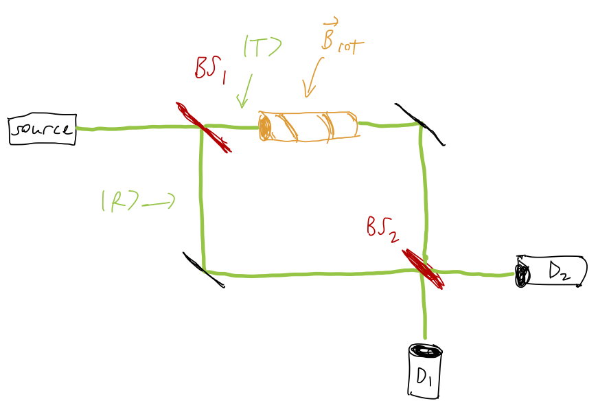
We hold a constant magnetic field |\vec{B}| over the whole experiment, but within the upper arm region the direction of the field is rotated in a plane, coming back to its starting point. This results in the dynamical phase due to the magnetic field being identical, so that the interference effect at the output of the interferometer depends purely on the Berry phase from the rotating-field region. What is striking about the result of this experiment is what doesn’t change the outcome; we can vary the strength of the magnetic field, or the speed at which the rotation happens, and the resulting detection probability remains identical. Only the path of the rotation - the size of the closed loop subtended by the rotation of the magnetic field - determines the Berry phase and thus the experimental outcome.
There are practical and interesting effects of the Berry phase in certain quantum systems, notably when studying band structure in crystals; it can also be used as a way to understand the quantum Hall effect. The mathematics is fairly deep, too (just the few things I’ve said already should remind you a lot of our discussions of gauge symmetry!) We won’t dig into either of these topics here, but I wanted to motivate that the Berry phase is more than just a curiosity. If you’re interested in the physics of the Berry phase, I give a little bit more detail in Appendix D.
Although it’s something of a side note, one simple observation we can make about the Berry phase is that it will be exactly zero in any system where we can take the wavefunctions to be purely real. This is somewhat intuitive; accumulating a phase through our evolution requires there to be a phase that our wavefunctions are sensitive to.
More concretely, we can prove that the Berry connection appearing in the geometric phase is zero if our states are purely real. The connection is proportional to \bra{E_n} \vec{\nabla}_\theta \ket{E_n}; we can start with the product rule instead to write \nabla_\theta (\left\langle E_n | E_n \right\rangle) = \bra{E_n} (\nabla_\theta \ket{E_n}) + (\nabla_\theta \bra{E_n}) \ket{E_n}. However, the left-hand side here is zero since \left\langle E_n | E_n \right\rangle = 1, while the two terms on the right-hand side are related by complex conjugation, so \bra{E_n} \nabla_\theta \ket{E_n} = -(\bra{E_n} \nabla_\theta \ket{E_n})^\star, or in other words, the real part of \bra{E_n} \nabla_\theta \ket{E_n} has to be zero. If the wavefunction is real, then the imaginary part is also zero, so the whole thing vanishes.