7 Time-evolution pictures and classical from quantum
7.1 Schrödinger and Heisenberg pictures
Now, let’s talk more generally about operator algebra and time evolution. So far, we have studied time evolution in the Schrödinger picture, where state kets evolve according to the Schrödinger equation i \hbar \frac{d}{dt} \ket{\psi(t)} = \hat{H} \ket{\psi(t)}, while operators (and thus basis kets) are time-independent. As we saw, when \hat{H} is time-independent, we can formally integrate this equation to obtain \ket{\psi(t)} = e^{-i \hat{H} t/\hbar} \ket{\psi(0)} \equiv \hat{U}(t) \ket{\psi(0)}, i.e. time evolution is just the result of a unitary operator \hat{U} acting on the kets.
There are some assumptions needed to write even the formal solution for \hat{U}(t) above; for example, we assume \hat{H} doesn’t depend on time. What about the more general case?
It turns out that time evolution can always be thought of as equivalent to a unitary operator acting on the kets, even when the Hamiltonian is time-dependent. First, suppose that \hat{H} depends explicitly on time but commutes with itself at different times, e.g. a spin-1/2 particle interacting with a background magnetic field whose direction is fixed but whose magnitude changes, \hat{H} = \frac{e}{mc} \hat{S_z} B_z(t). Here we can still solve the Schrödinger equation just by formally integrating both sides, but now that \hat{H} depends on time we end up with an integral in the exponential, \hat{U}(t) = \exp \left[ - \left(\frac{i}{\hbar}\right) \int_0^t dt'\ \hat{H}(t') \right]. There exist even more complicated cases where the Hamiltonian doesn’t even commute with itself at different times. In fact, we just saw such an example; the spin-1/2 particle in a magnetic field which rotates in the xy plane gives a Hamiltonian such that [\hat{H}(t), \hat{H}(t')] \neq 0. There is, nevertheless, still a formal solution known as the Dyson series, \hat{U}(t) = 1 + \sum_{n=1}^\infty \left( \frac{-i}{\hbar} \right)^n \int_0^t dt_1 \int_0^{t_1} dt_2 ... \int_0^{t_{n-1}} dt_n \hat{H}(t_1) \hat{H}(t_2)...\hat{H}(t_n). (This is a good time to appreciate the fact that we didn’t have to use the formal solution for the two-state system!) It’s not self-evident that these more complicated constructions are still unitary, especially the Dyson series, but rest assured that they are. So time evolution is always a unitary transformation acting on the states.
As we observed before, this implies that inner products of state kets are preserved under time evolution: \left\langle \alpha(t) | \beta(t) \right\rangle = \bra{\alpha(0)} \hat{U}{}^\dagger(t) \hat{U}(t) \ket{\beta(0)} = \left\langle \alpha(0) | \beta(0) \right\rangle. On the other hand, the matrix elements of a general operator \hat{A} will be time-dependent, unless \hat{A} commutes with \hat{U}: \bra{\alpha(t)} \hat{A} \ket{\beta(t)} = \bra{\alpha(0)} \hat{U}{}^\dagger(t) \hat{A} \hat{U}(t) \ket{\beta(0)} Notice that by definition in the Schrödinger picture, the unitary transformation only affects the states, so the operator \hat{A} remains unchanged. But now, we can see that we could have equivalently left the state vectors unchanged, and evolved the observable in time, i.e. \bra{\alpha} \hat{A}(t) \ket{\beta} = \bra{\alpha} (\hat{U}{}^\dagger (t) \hat{A}(0) \hat{U}(t)) \ket{\beta}. This is exactly the same product of states and operators; we get the same answer. But now all of the time dependence has been pushed into the observable. This is the Heisenberg picture of quantum mechanics.
Which picture is better to work in? There’s no definitive answer; the two pictures are useful for answering different questions. In particular, we might guess that the Heisenberg picture would make it easier to connect with classical mechanics; in the classical world, observables themselves (things like position \vec{x} or angular momentum \vec{L}) are the things which evolve in time, whereas there’s no classical analogue to the state vector.
Let’s make our notation explicit. We define the Heisenberg picture observables by \hat{A}{}^{(H)}(t) \equiv \hat{U}{}^\dagger(t) \hat{A}{}^{(S)} \hat{U}(t), where (H) and (S) stand for Heisenberg and Schrödinger pictures, respectively. The two operators are equal at t=0, by definition; \hat{A}{}^{(S)} = \hat{A}(0). Here (and in many other references), an operator appearing with no picture label and no time dependence is assumed to be Schrödinger picture, i.e. \hat{A} = \hat{A}{}^{(S)}, although for this section I’ll try to use explicit Schrödinger labels for clarity. On the other hand, in the Heisenberg picture the state vectors are frozen in time, \ket{\alpha(t)}_H = \ket{\alpha(0)} whereas in the Schrödinger picture we have \ket{\alpha(t)}_S = \hat{U}(t) \ket{\alpha(0)}. As we’ve observed, expectation values are the same, no matter what picture we use, as they should be (the choice of picture itself is not physical.)
We can derive an equation of motion for the operators in the Heisenberg picture, starting from the definition above and differentiating: \frac{d\hat{A}{}^{(H)}}{dt} = \frac{d\hat{U}{}^\dagger}{dt} \hat{A}{}^{(S)} \hat{U} + \hat{U}{}^\dagger \hat{A}{}^{(S)} \frac{d \hat{U}}{dt} \\ = -\frac{1}{i\hbar} \hat{H} \hat{U}{}^\dagger \hat{A}{}^{(S)} \hat{U} + \frac{1}{i\hbar} \hat{U}{}^\dagger \hat{A}{}^{(S)} \hat{U} \hat{H} \\ \Rightarrow \frac{d \hat{A}{}^{(H)}}{dt} = \frac{1}{i\hbar} [\hat{A}{}^{(H)}, \hat{H}]. This is the Heisenberg equation of motion, and I’ve made use of the fact that the unitary operator \hat{U}, which is constructed from \hat{H}, certainly commutes with \hat{H}.
We have assumed above that the Schrödinger picture operator \hat{A}^{(S)} is time-independent, but sometimes we want to include explicit time dependence of an operator, e.g. a time-varying external magnetic field. In this case, the complete Heisenberg equation of motion should be written \frac{d\hat{A}{}^{(H)}}{dt} = \frac{1}{i\hbar} [\hat{A}{}^{(H)}, \hat{H}] + \left(\frac{\partial \hat{A}}{\partial t}\right)^{(H)}
where the last term is related to the Schrödinger picture operator like so: \left(\frac{\partial \hat{A}}{dt}\right)^{(H)} = \hat{U}{}^\dagger \frac{\partial \hat{A}{}^{(S)}(t)}{\partial t} \hat{U}.
Notice that the operator \hat{H} itself doesn’t evolve in time in the Heisenberg picture. (Assuming it has no explicit time dependence, and Heisenberg picture can become very messy if it does!) Likewise, any operators which commute with \hat{H} are time-independent in the Heisenberg picture.
Actually, this equation requires some explaining, because it immediately contravenes my definition that “operators in the Schrödinger picture are time-independent”. The more correct statement is that “operators in the Schrödinger picture do not evolve in time due to the Hamiltonian of the system”; we have to separate out the time-dependence due to the Hamiltonian from explicit time dependence (again, most commonly imposed by the presence of a time-dependent background classical field.)
7.1.1 Evolution of basis kets
In the Schrödinger picture, our starting point for any calculation was always with the eigenkets of some operator, defined by the equation \hat{A}{}^{(S)} \ket{a}_S = a \ket{a}_S. The eigenkets \ket{a} then give us part or all of a basis for our Hilbert space. Since the operator doesn’t evolve in time, neither do the basis kets. On the other hand, since the Heisenberg-picture operators do evolve in time, their eigenkets must as well: \hat{A}{}^{(H)}(t) \ket{a,t}_H = a \ket{a,t}_H. (Remember that the eigenvalues are always the same, since a unitary transformation doesn’t change the spectrum of an operator!) Expanding out in terms of the operator at time zero, \hat{A}{}^{(H)}(0) \ket{a,0} = a \ket{a,0} \\ \hat{U}{}^\dagger (t) \hat{A}{}^{(H)}(0) (\hat{U}(t) \hat{U}{}^\dagger) \ket{a,0} = a \hat{U}{}^\dagger (t) \ket{a,0} where I’ve inserted the identity operator. But now we can see the Heisenberg picture operator at time t on the left-hand side, and we identify the evolution of the ket, \ket{a,t}_H = \hat{U}{}^\dagger (t) \ket{a,0}. This is the opposite direction of how the state evolves in the Schrödinger picture, and in fact the eigenstate kets satisfy the Schrödinger equation with the wrong sign, i \hbar \frac{\partial}{\partial t} \ket{a,t}_H = - \hat{H} \ket{a,t}_H.
This starts to get confusing if we are using an operator to define a basis, which we often do in quantum mechanics! Suppose we have a state vector that we have expanded out in the eigenbasis of \hat{A} at time zero: \ket{\psi(0)} = \sum_{a} c_\psi(a) \ket{a} where c_\psi(a) = \left\langle a | \psi \right\rangle. In the Schrödinger picture, the basis states are fixed, and so to include time evolution we just have to make the coefficients c_\psi(a) time-dependent: \ket{\psi(t)}^{(S)} = \sum_{a} c_\psi^{(S)}(a,t) \ket{a}_S which is straightforward. In the Heisenberg picture, our basis changes but the state vector is fixed - which means the coefficients of the expansion are still time-dependent: \ket{\psi}^{(H)} = \sum_{a} c_\psi^{(H)}(a,t) \ket{a,t}_H in such a way that the time dependence must cancel between the c_\psi^{(H)} and the \ket{a,t}_H!
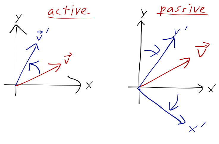
If this seems completely bizarre, an analogy back to ordinary vector spaces might help here. We can think of a unitary transformation like the time-evolution operator as a rotation acting on the kets (vectors) in our Hilbert space. In Schrödinger picture, time evolution is an active transformation; we begin with a state vector at t=0, and the rotation maps it to a new state vector. Heisenberg picture, on the other hand, is a passive transformation: the state vector is kept fixed and we rotate the coordinate system (the eigenbasis kets) around in the opposite direction. The end result is the same.
Just to drive the point home, if we ask a good, physical question, like “what is the probability amplitude for the system which exists in state \ket{\psi} at t=0 to be observed in an eigenstate \ket{b} of operator \hat{B} at time t”, then the answer in the Schrödinger picture is p(b,t) = \left\langle b | \psi(t) \right\rangle = \bra{b} \left( e^{-i\hat{H} t/\hbar} \ket{\psi(0)} \right), while in the Heisenberg picture, it is the same thing with a different association: p(b,t) = \left\langle b(t) | \psi \right\rangle = \left( \bra{b} e^{-i\hat{H} t/\hbar} \right) \ket{\psi(0)}.
7.2 Evolution of expectation values and Ehrenfest’s theorem
The Heisenberg equation of motion provides a simple and direct way to connect back to classical mechanics, which must of course emerge from quantum mechanics. The time evolution of a classical system can be written in the familiar-looking form \frac{dA}{dt} = \{A, H\}_{PB} + \frac{\partial A}{\partial t} where H is the Hamiltonian, and the brackets are the Poisson bracket, defined in general as \{f, g\}_{PB} = \sum_i \left( \frac{\partial f}{\partial q_i} \frac{\partial g}{\partial p_i} - \frac{\partial f}{\partial p_i} \frac{\partial g}{\partial q_i}\right). So the Heisenberg equation of motion can be obtained from the classical one by applying Dirac’s quantization rule, \{,\}_{PB} \rightarrow \frac{1}{i\hbar} [,]. This approach, known as canonical quantization, was one of the early ways to try to understand quantum physics. You should be suspicious about the claim that we can derive quantum mechanics from classical mechanics, and in fact we know that we can’t; operators like spin have no classical analogue from which to start. (There are other, more subtle issues; in fact the quantization rule fails even for some observables that do have classical counterparts, if they involve higher powers of \hat{x} and \hat{p} for instance.)
Let’s have a closer look at some of the parallels between classical mechanics and QM in the Heisenberg picture. First, a useful identity between \hat{x} and \hat{p}: it’s straightforward to show that \begin{aligned} [\hat{x}, \hat{p}^n] &= ni\hbar \hat{p}^{n-1}, \\ [\hat{p}, \hat{x}^n] &= -ni\hbar \hat{x}^{n-1}. \end{aligned}
Derive the commutator identity for [\hat{x}, \hat{p}^n] above. (You can try [\hat{p}, \hat{x}^n] as well - the algebra is largely the same.)
Answer:
We can start by splitting up \hat{p}^n and then using a commutator identity:
[\hat{x}, \hat{p}^n] = [\hat{x}, \hat{p} \hat{p}^{n-1}] \\ = \hat{p} [\hat{x}, \hat{p}^{n-1}] + [\hat{x}, \hat{p}] \hat{p}^{n-1} \\ = \hat{p} [\hat{x}, \hat{p}^{n-1}] + i\hbar \hat{p}^{n-1}.
If we do the same trick again, (...) = \hat{p} \left( \hat{p} [\hat{x}, \hat{p}^{n-2}] + i\hbar \hat{p}^{n-2}\right) + i\hbar \hat{p}^{n-1} \\ = \hat{p}{}^2 [\hat{x}, \hat{p}^{n-2}] + 2i\hbar \hat{p}^{n-1} and so on. Expansion of the commutator will terminate at [\hat{x}, \hat{p}] = i\hbar, at which point there will be (n-1) copies of the i\hbar \hat{p}{}^{n-1} term, plus one copy from the initial term with the commutator - leaving us with n times this term, verifying the identity.
These can be used with the power-series definition of functions of operators to derive the even more useful identities below:
For the position and momentum operators, commutators involving functions of position and momentum simplify as follows: \begin{aligned} [\hat{x}, F(\hat{p})] &= i \hbar \frac{\partial F}{\partial \hat{p}}, \\ [\hat{p}, G(\hat{x})] &= -i \hbar \frac{\partial G}{\partial \hat{x}}. \end{aligned}
There’s an important subtlety that I’ve glossed over: now that our operators are functions of time, we have to be careful with how the commutation relations between them are altered. In particular, the canonical commutation relation [\hat{x}(0), \hat{p}(0)] = i\hbar is now only guaranteed to be true for the original operators at t=0. Actually, it is a bit more general than that. Let’s consider the commutator at the same time t: [\hat{x}(t), \hat{p}(t)] = \hat{x}(t) \hat{p}(t) - \hat{p}(t) \hat{x}(t) \\ = \hat{U}^\dagger(t) \hat{x} \hat{U}(t) \hat{U}^\dagger(t) \hat{p} \hat{U(t)} - \hat{U}^\dagger(t) \hat{p} \hat{U}(t) \hat{U}^\dagger(t) \hat{x} \hat{U(t)} \\ = \hat{U}^\dagger(t) [\hat{x}, \hat{p}] \hat{U}(t) \\ = \hat{U}^\dagger(t) (i\hbar) \hat{U}(t) = i\hbar. So in fact, the simple commutation relation does hold in the Heisenberg picture, as long we the two operators are evaluated at the same time. The appropriate jargon is that [\hat{x}, \hat{p}] = i\hbar is said to be an equal-time commutation relation.
On the other hand, if we’re at different times, it’s now possible that our operators don’t even commute with themselves: i.e. in general, [\hat{x}(t), \hat{x}(0)] \neq 0.
Before we continue, it’s useful to make a remark about the commutator on the right-hand side of the Heisenberg equation. Formally, the Heisenberg equation is a differential equation, which means we have no way of evaluating the commutator [\hat{A}^{(H)}(t), \hat{H}]. However, since \hat{H} commutes with time evolution, we can relate this commutator directly to the commutator at zero time: [\hat{A}(t), \hat{H}] = \hat{A}(t) \hat{H} - \hat{H} \hat{A}(t) \\ = \hat{U}^\dagger(t) \hat{A} \hat{U}(t) \hat{H} - \hat{H} \hat{U}^\dagger(t) \hat{A} \hat{U}(t) \\ = \hat{U}^\dagger(t) (\hat{A} \hat{H} - \hat{H} \hat{A}) \hat{U}(t) \\ = \hat{U}^\dagger(t) [\hat{A}, \hat{H}] \hat{U}(t). So commutators with the Hamiltonian are time-independent: [\hat{A}(0), \hat{H}] = \hat{B}(0) \Rightarrow [\hat{A}(t), \hat{H}] = \hat{B}(t). In other words, we can treat the Hamiltonian as being defined using the operators at any time t and then apply equal-time commutation relations. (This makes intuitive sense, since \hat{H} doesn’t depend on time itself, so it shouldn’t matter what time we define it at!)
From here forward I’ll skip the (H) superscripts and work explicitly in Heisenberg picture only. Before we treat the general case, it’s worth considering the time evolution for the free case, \hat{H}_0 = \hat{p}{}^2/2m. Here, the momentum commutes with \hat{H}, which means that it is conserved: \frac{d\hat{p}}{dt} = \frac{1}{i\hbar} [\hat{p}, \hat{H}_0] = 0.
The position operator evolution will be non-trivial, but still simple and consistent with classical expectations for a free particle.
Here, you should complete Tutorial 4 on “Time evolution of position and momentum operators”. (Tutorials are not included with these lecture notes; if you’re in the class, you will find them on Canvas.)
Now let’s study the full case with an arbitrary potential, \hat{H} = \frac{\hat{p}^2}{2m} + V(\hat{x}). For the position evolution, using the identities above we find: \frac{d\hat{x}}{dt} = \frac{1}{i\hbar} [\hat{x}, \hat{H}] \\ = \frac{1}{2mi\hbar} \left(i\hbar \frac{\partial \hat{H}}{\partial \hat{p}}\right) \\ = \frac{\hat{p}}{m}. This is exactly the classical definition of the momentum for a free particle, and the “trajectory” as a function of time looks like a classical trajectory: x(t) = x(0) + \left( \frac{p(0)}{m}\right) t.
Now, we switch back on the potential function V(\hat{x}). This doesn’t change our time-evolution equation for the \hat{x}, since they commute with the potential. However, for the momentum operators, we now have \frac{d\hat{p}}{dt} = \frac{1}{i\hbar} [\hat{p}, V(\hat{x})] = -\frac{\partial V}{\partial x}. This should already look familiar, and if we go back and take the time derivative of the dx/dt expression above, we can eliminate the momentum to rewrite it in the more familiar form m \frac{d^2 \hat{x}}{dt^2} = - \frac{\partial V(\hat{x})}{\partial x}. This is (the quantum version of) Newton’s second law! This derivation depended on the Heisenberg picture so it isn’t quite physical yet, but if we take expectation values then we find a picture-independent statement, which I’ll write in its full three-dimensional form:
For a quantum particle of mass m with Hamiltonian \hat{H} = \frac{\hat{\vec{p}}^2}{2m} + V(\hat{\vec{x}}), the time evolution of position and momentum expectation values obey the equation m \frac{d^2}{dt^2} \left\langle \hat{\vec{x}} \right\rangle = \frac{d}{dt} \left\langle \hat{\vec{p}} \right\rangle = - \left\langle \nabla V(\hat{\vec{x}}) \right\rangle.
This was derived by Ehrenfest using wave mechanics; we had a much easier path with the Heisenberg picture, which makes it more or less obvious once we write down the operator time evolution. In particular, if we consider a quantum wave packet, Ehrenfest’s theorem tells us that on average, the center of the wave packet moves exactly like a classical particle.
7.3 Example: time evolution of the SHO
Back to the simple harmonic oscillator: \hat{H} = \frac{\hat{p}{}^2}{2m} + \frac{1}{2} m \omega^2 \hat{x}{}^2 Let’s see how the SHO evolves in time using the Heisenberg picture. The equations of motion for the position and momentum operators are \frac{d\hat{p}}{dt} = \frac{1}{i\hbar} [\hat{p}, \hat{H}] = - m\omega^2 \hat{x} \\ \frac{d\hat{x}}{dt} = \frac{1}{i\hbar} [\hat{x}, \hat{H}] = \frac{\hat{p}}{m}, mimicking the classical equations of motion. On to the ladder operators; we could compute their time evolution directly, but since we did it for \hat{p} and \hat{x} already let’s just use the change of variables, \frac{d\hat{a}}{dt} = \sqrt{\frac{m\omega}{2\hbar}} \left( \frac{\hat{p}}{m} + \frac{i}{m \omega} (-m \omega^2 \hat{x}) \right) \\ = -i \omega \hat{a}, \\ \frac{d\hat{a}{}^\dagger}{dt} = i \omega \hat{a}{}^\dagger. These are nice and easy to solve: \hat{a}(t) = e^{-i\omega t} \hat{a}(0) \\ \hat{a}{}^\dagger (t) = e^{i \omega t} \hat{a}{}^\dagger(0). It’s easy to see that the number operator \hat{N} = \hat{a}{}^\dagger \hat{a} is time-independent, which it should be since it commutes with \hat{H}. Working backwards with our definitions of \hat{x} and \hat{p} in terms of the ladder operators, we find that \hat{x}(t) = \hat{x}(0) \cos \omega t + \frac{\hat{p}(0)}{m\omega} \sin \omega t \\ \hat{p}(t) = - m \omega \hat{x}(0) \sin \omega t + \hat{p}(0) \cos \omega t So the quantum observables oscillate at frequency \omega, just like their classical counterparts.
There’s another way to derive these results which is instructive. Instead of using the ladder operators, we can just attempt to directly evaluate the time evolution operator, i.e. \hat{x}(t) = e^{i\hat{H} t/\hbar} \hat{x}(0) e^{-i \hat{H} t/\hbar}. and similarly for \hat{p}(t). There is a very nice formula for operators sandwiched between exponentials like this that is often useful:
If \hat{A} and \hat{G} are Hermitian operators, then: e^{i\hat{G} \lambda} \hat{A} e^{-i\hat{G} \lambda} = \hat{A} + i \lambda [\hat{G}, \hat{A}] - \frac{\lambda^2}{2} [\hat{G}, [\hat{G}, \hat{A}] ] + ... \\ \ + \left( \frac{i^n \lambda^n}{n!} \right) [\hat{G}, [\hat{G}, [\hat{G}, ...[\hat{G}, \hat{A}] ] ]...] + ...
Because this is an infinite sum, it’s not useful unless there is either a pattern in the commutators, or we truncate the series by hand (useful for perturbation in a small quantity.) The commutation relations of the SHO Hamiltonian at t=0 happen to give rise to a repeating structure: \begin{aligned} [\hat{H}, \hat{x}(0)] &= -\frac{i \hbar}{m} \hat{p}(0) \\ [\hat{H}, \hat{p}(0)] &= i \hbar m \omega^2 \hat{x}(0). \end{aligned} Similar to our previous example with the Pauli matrices, these relations let us split the infinite Baker-Hausdorff series into a pair of power series in ordinary numbers, multiplying the two operators \hat{x}(0) and \hat{p}(0). You should be able to see that the two power series are exactly the trigonometric functions, and so e^{i\hat{H} t/\hbar} \hat{x}(0) e^{-i\hat{H} t/\hbar} = \hat{x}(0) \cos \omega t + \frac{\hat{p}(0)}{m \omega} \sin \omega t, exactly as we found above (and the same setup will work for \hat{p}(t), obviously.)
If we take expectation values, does the quantum harmonic oscillator behave just like the classical counterpart, i.e. with \left\langle \hat{x} \right\rangle \propto \sin \omega t and similar for \left\langle \hat{p} \right\rangle? Well, yes and no. In fact, if we take our state vector to be a pure energy eigenstate \ket{\psi} = \ket{n}, then we find that both expectation values are zero at t=0: \left\langle \hat{x}(0) \right\rangle = \left\langle \hat{p}(0) \right\rangle = 0 In fact, it’s easy to see in either picture that the expectation values are zero for all time; in Schrödinger picture the energy eigenstates don’t evolve except for a phase, and in Heisenberg picture we can think of the evolution cancelling between the basis kets and the operators (try not to get confused by the state ket being equal to a basis ket at t=0 here.) This doesn’t contradict Ehrenfest’s theorem, since we find that m \frac{d^2 \left\langle \hat{x} \right\rangle}{dt^2} = -\left\langle \nabla V(x) \right\rangle = -\left\langle m\omega^2 \hat{x} \right\rangle = 0.
Of course, these are energy eigenstates, which makes them somewhat delocalized and hard to think about in analogy to classical mechanics. For a better classical analogue, we should consider the coherent states \ket{\alpha} that we introduced previously. What happens to a coherent state under time evolution? We know we can write them as \ket{\alpha} = e^{-|\alpha|^2/2} e^{\alpha \hat{a}^\dagger} \ket{0}
Under time evolution we know that \hat{a}^\dagger(t) = e^{i\omega t} \hat{a}^\dagger(0). We can just absorb this into the time evolution of the eigenvalue \alpha; to be explicit, we write \alpha \hat{a}^\dagger(t) = \alpha e^{i \omega t} \hat{a}^\dagger(0) = (\alpha(t)) \hat{a}^\dagger(0) letting \alpha(t) = e^{i\omega t} \alpha(0). Then \ket{\alpha(t)} = e^{-|\alpha(0)|^2/2} e^{\alpha(t) \hat{a}^\dagger} \ket{0} \\ = \ket{e^{i \omega t} \alpha(0)}. (One minor detail: notice that since the time evolution comes from the operator, the normalization term remains as |\alpha(0)|^2. But since \alpha(t) is evolving by a pure phase, |\alpha(t)|^2 = |\alpha(0)|^2. Also, keep in mind this is Heisenberg picture evolution of a state, so you may see extra factors if you look in a different picture…)
The key feature here is that our coherent state remains as a coherent state, so it does not spread out as time evolves, remaining a minimum-uncertainty state with \Delta x = \hbar / (2m \omega). The state itself isn’t physical (depends on the picture), but the minimum uncertainty can be verified by explicitly calculating expectation values. Speaking of which, we can read off the time-evolved values of position and momentum: if we let \alpha(0) give us some initial position x_0 and initial momentum p_0, then \left\langle \hat{x}(t) \right\rangle = \sqrt{\frac{2\hbar}{m\omega}} {\rm Re}(\alpha) = x_0 \cos (\omega t), \\ \left\langle \hat{p}(t) \right\rangle = \sqrt{2\hbar m \omega} {\rm Im}(\alpha) = p_0 \sin (\omega t). So our coherent state evolves exactly as we would expect for a classical point particle in a harmonic oscillator potential (as it had to, thanks to Ehrenfest’s theorem.)
7.4 The interaction picture
The difference between Schrödinger picture and Heisenberg picture, as we have seen, is just a matter of organization: whether we prefer to keep the time evolution operator \hat{U} with the state kets or with the basis kets. There is another, more complicated possibility, which is that we can divide up the time evolution and assign part of it to both.
Why would we ever do such a thing? The best reason is to work in a specific third picture, called the interaction picture. Here, we start by dividing up the Hamiltonian into a piece which is time-independent and relatively simple, and “everything else”: \hat{H} = \hat{H}_0 + \hat{V} The choice of what \hat{H}_0 is depends on the problem we’re solving. Following this division, we define a partial time-evolution operator \hat{U}_0(t) \equiv \exp \left( \frac{i\hat{H}_0 t}{\hbar} \right) (note the minus sign relative to the usual Schrödinger picture operator!) We then define the interaction-picture states from the Schrödinger picture states as \ket{\psi(t)}_I = \hat{U}_0(t) \ket{\psi(t)}_S. Because of the minus sign in the definition of \hat{U}_0(t), the effect of this definition is to “subtract” the piece of the Schrödinger time evolution that comes from the simple part \hat{H}_0. By doing so, in order to keep matrix elements invariant, we have introduced some time evolution into our operators: we must have \hat{O}{}^{(I)}(t) = e^{i\hat{H}_0 t/\hbar} \hat{O} e^{-i\hat{H}_0 t/\hbar} = \hat{U}_0(t) \hat{O} \hat{U}_0^\dagger(t).
How do the interaction-picture states evolve in time? We can apply the Schrödinger equation to the original states: i \hbar \frac{\partial}{\partial t} \ket{\psi(t)}_I = -\hat{H}_0 e^{i\hat{H}_0 t/\hbar} \ket{\psi(t)}_S + e^{i\hat{H}_0 t/\hbar} \left( i \hbar \frac{\partial}{\partial t} \ket{\psi(t)}_S \right) \\ = -\hat{H}_0 \ket{\psi(t)}_I + e^{i \hat{H}_0 t/\hbar} (\hat{H}_0 + \hat{V}) \ket{\psi(t)}_S \\ = - \hat{H}_0 \ket{\psi(t)}_I + (\hat{H}_0 + e^{i\hat{H}_0 t/\hbar} \hat{V} e^{-i\hat{H}_0 t/\hbar}) \ket{\psi(t)}_I \\ = \hat{V}{}^{(I)} \ket{\psi(t)}_I. So the interaction-picture states evolve according to the Schrödinger equation, but with the full Hamiltonian replaced with just the terms contained in \hat{V}. Meanwhile, our definition of the operators above indicates that they evolve according to the Heisenberg equation, but with the other piece \hat{H}_0: \frac{d \hat{O}{}^{(I)}}{dt} = \frac{1}{i\hbar} [\hat{O}{}^{(I)}, \hat{H}_0] + \left( \frac{\partial \hat{O}}{\partial t} \right)^{(I)}, where again as in the Heisenberg picture we have to be careful to separate out both kinds of time dependence in the last term: here, \left(\frac{\partial \hat{O}}{\partial t}\right)^{(I)} = \hat{U}_0(t) \frac{\partial \hat{O}{}^{(S)}}{\partial t} \hat{U}_0^\dagger(t).
We won’t see the interaction picture much more this semester, but it is extremely important, particularly for time-dependent perturbation theory, where all of the small time-dependent terms are gathered in \hat{V}, separated out from the simple time-independent evolution dictated by \hat{H}_0. Being able to rely on a complete analytic solution for the spectrum of \hat{H}_0 is often an excellent starting point to understand the more complex system with \hat{V} included. In quantum field theory (fully relativistic QM), the interaction picture is used almost exclusively, separating out the simple propagation of free particles and their interactions, which are treated perturbatively.