26 Gauge symmetry
We’re now equipped to deal with a more subtle kind of symmetry, known as gauge symmetry. A gauge transformation, generally, can be thought of as a redefinition of the potential energy. Our main goal will be electromagnetic gauge symmetry, but let’s start with a much simpler version, which will still turn out to give interesting results in quantum systems.
26.1 Potential energy and phase shifts
The simplest example of a gauge transformation is simply adding a constant to our potential energy, \tilde{V}(\vec{x}) = V(\vec{x}) + V_0, where V_0 is constant in both space and time. You can think of this as simply a redefinition of what we call the zero-point of energy, hence the name “gauge transformation” (we would have to relabel the “gauge” we use to measure V(x).)
Classically, adding a constant to our definition of potential has no effect at all on the physics; in terms of Newton’s laws, the force depends only on the gradient of the potential, so we can add any constant we want.
Is the same statement true in quantum mechanics? We might be worried that it won’t be, since if we look at the time-independent Schrödinger equation, we notice that the potential appears directly, without any derivative: -\frac{\hbar^2}{2m} \nabla^2 \psi + (V(\vec{x}) - E) \psi(\vec{x}) = 0. In fact, changing from V to \tilde{V} will affect the time evolution of our kets: we see that from some initial ket \ket{\alpha}, we will find with the new potential \tilde{\ket{\alpha, t}} = \exp \left[ -i \left( \frac{\vec{p}^2}{2m} + V(\vec{x}) + V_0\right) \frac{t}{\hbar} \right] \ket{\alpha} \\ = e^{-iV_0 t/\hbar} \ket{\alpha, t}. So changing the zero of the potential changes our definition of the time-evolved ket by a phase. If \alpha is an energy eigenstate, then e^{-iV_0 t/\hbar} \ket{\alpha,t} = \exp \left( \frac{-i(E+V_0)t}{\hbar} \right) \ket{\alpha}. Thus, all we’ve done is replaced E \rightarrow E + V_0, as we should expect. In fact, nothing we can actually observe has changed; rescaling every ket in the Hilbert space by the same phase leaves all inner products and expectation values unchanged (as we’ve observed before.)
Although we have seen that a completely global rescaling of the potential energy has no physical effect, there are some rather large surprises lurking in the effects of local potential changes in quantum mechanics. As a first taste of this subject, consider an experiment involving two metallic cages, which are maintained at a constant potential difference. We take a beam of electrons and split it into two parts to pass through the two cages:
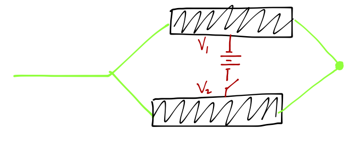
We switch the potential difference on only while the electrons are in the cages, so they never feel an electric force outside the cages. Within each cage, the electric potential is uniform, and so the particles again feel no force. However, there is a phase shift induced by the background potential, and the phase shift is different in each cage. Thus, if we recombine the beams at the other end of the cages, we find that the measured intensity of the recombined beam exhibits interference, with the intensity modulating according to the difference in phase shifts, I \sim \cos \left( \frac{1}{\hbar} \int dt\ [V_2(t) - V_1(t)] \right) You’ll notice from the presence of \hbar that this is a purely quantum mechanical effect, which vanishes as \hbar \rightarrow 0 and the oscillations become infinitely fast. This is a first example of something which we will see in detail: although only the electromagnetic fields are “real” in classical theory, in quantum theory the electromagnetic potential fields themselves are more fundamental.
A slightly more elaborate but much more interesting example is given by an experiment known as the gravity interferometer. Rather famously, the unification of gravity and quantum mechanics is an unsolved problem to this day, but there are still quantum-mechanical effects that can be observed and explained perfectly in the presence of a background, classical gravitational field.
In classical mechanics, gravity is usually the first force which is encountered, partly because it is so simple to deal with: the classical equation of motion for a particle in the Earth’s gravitational field is simply \vec{F} = m\ddot{z} = -mg and the mass cancels out, leaving a constant acceleration. What about the quantum system? Again for a particle moving in one dimension, we have \left[ - \left( \frac{\hbar^2}{2m}\right) \frac{d^2}{dz^2} + m\Phi_g \right] \psi(z) = i\hbar \frac{\partial \psi}{\partial t}. where \Phi_g = gz is the (approximate) gravitational potential field near the Earth’s surface. Now the mass doesn’t cancel; the best we can do is divide through, so that our equation depends only on the ratio \hbar/m. (Putting the gravitational action into the path integral leads to a similar conclusion, that we can’t get rid of \hbar/m.)
This is a simple aside elaborating on the remark above: why does dependence on m cancel classically but not quantum mechanically? If we take the classical gravitational action near the Earth’s surface, in the quantum system, the action appears in the path integral as \left\langle z_f, t_f | z_i, t_i \right\rangle = \int \mathcal{D}[z(t)] \exp \left[ i \int_{t_i}^{t_f} dt \frac{1}{\hbar} \left( \frac{1}{2} m\dot{z}^2 - mgz \right) \right] which again depends on \hbar/m, and in particular we can’t factor out the mass in any way. On the other hand, for the classical action we’re only interested in the stationary point \delta \int_{t_i}^{t_f} dt \left( \frac{1}{2} m\dot{z}^2 - mgz \right) = 0 and we can just divide both sides by m before we do the variation.
Of course, to first order the behavior of a quantum particle in a classical gravity field will just be free-fall, i.e. \frac{d^2 \left\langle z \right\rangle}{dt^2} = -g. (This can be derived from the Schrödinger equation.) To really see a quantum effect, we want to find some explicit dependence on \hbar/m, which we can obtain with the right experiment. As I mentioned, a gravitational interferometer is the best example. Like the electric field example above, we prepare a beam of neutrons and split it along two different paths, A \to B \to D and A \to C \to D:
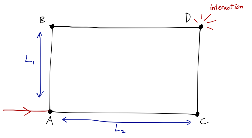
This is sort of a gravitational analogue of the experiment with the electrons and cages above. We imagine that the experiment is mounted on an adjustable platform, so that we can change the angle of gravity relative to the paths. If the plane of the paths is perfectly horizontal, then there is no effect, since the gravitational potential is constant everywhere. However, if we tilt to an angle \delta along the axis parallel to AC, then path BD is at a higher potential than AC by an amount \Delta V = m_n g L_2 \sin \delta. The potential changes in the same way for traversing paths AB and CD, so only the above potential difference is significant, and it leads to a phase shift at the interference point of \Delta \phi = \frac{m_n g L_2 (\sin \delta) T}{\hbar} where T is the time-of-flight (with the actual probability at the detector going as \cos^2 (\Delta \phi), just like the double-slit interference experiment.) This is now an \hbar/m effect, and the dimensions actually work out nicely for a tabletop experiment; this formula was confirmed by just such an experiment in 1975, which you can see in Sakurai. Notice that just like the electron beam experiment, we are sensitive in quantum mechanics directly to the potential \Phi_g through the height difference (\sim \sin \delta), even though the gravitational acceleration itself is perfectly uniform even when we tilt the experiment.
One other aside before we keep moving: one of the reasons that we can cancel out the mass dependence in classical mechanics is the equivalence principle, i.e. the equality of inertial mass (the one that appears in F=ma) and gravitational mass. The m_n in the above formula is the gravitational mass, but the time-of-flight T depends on the inertial mass of the neutron, so we can think of the gravitational interferometer experiment as a test of the EP for a quantum-mechanical system.
The gravity interferometer experiment, while interesting, is a rather superficial test of how quantum mechanics and gravity interact; gravity only really appears as a static background field. You may have heard from other places that it is very hard to come up with a fully quantum theory of gravity, which is true. There are various reasons (which I won’t go into here) why quantum gravity is such a difficult problem, but it doesn’t help that it is very difficult to come up with good experimental tests, simply because gravity is by far the weakest force of nature.
Sakurai points to the example of a hydrogen atom, in which an electron and proton are bound by the electromagnetic force; the approximate size of the atom is given by the Bohr radius, a_0 = \frac{\hbar^2}{e^2 m_e} \approx 0.053\ {\rm nm} If we tried to construct a similar “atom” from a neutron and electron, bound only by the gravitational force, the equivalent “Bohr radius” would be a_{0,g} = \frac{\hbar^2}{G_N m_e^2 m_n} \sim 10^{13}\ {\rm ly} which is (substantially) larger than the size of the entire universe!
26.2 The electromagnetic potential
As you know, potentials don’t just appear as simple functions V(x); the electric and magnetic fields depend on both a scalar potential \phi, and a vector potential \vec{A}. Once again, we know that classical EM fields are invariant under certain redefinitions of these potentials, in particular \phi \rightarrow \phi + \frac{\partial f}{\partial t} \\ \vec{A} \rightarrow \vec{A} - \nabla f where f(\vec{x}, t) is some function of position and time in general. Once again, we will find that the potential functions themselves are important in the quantum theory.
Let’s start from the classical Hamiltonian for a charged particle in an electromagnetic field: H = \frac{1}{2m} \left( \vec{p} - \frac{q}{c} \vec{A}(\vec{x}) \right)^2 + q\phi(\vec{x}). This is simply a function of position and momentum, so to obtain the quantum Hamiltonian we just replace p and x with their operator counterparts. This is easier said than done, because now we have an ambiguity: there are multiple possible definitions of (p - qA/c)^2 involving products of \hat{\vec{p}} and \hat{\vec{A}} in different orders. We should certainly choose a Hermitian combination: let’s take the choice \hat{\vec{p}}{}^2 + \frac{q^2}{c^2} \hat{\vec{A}}{}^2 - \frac{q}{c} \left( \hat{\vec{p}} \cdot \hat{\vec{A}} + \hat{\vec{A}} \cdot \hat{\vec{p}} \right). We’ll start in the Heisenberg picture. Our first speed bump occurs in the time evolution of the \hat{\vec{x}} operator: for each component x_i we find \frac{d\hat{x}_i}{dt} = \frac{1}{i\hbar} [\hat{x}_i, \hat{H}] = \frac{1}{m} (\hat{p}_i - q\hat{A}_i/c). So m d\hat{x}_i / dt \neq \hat{p}_i! We define this new combination to be the kinematical momentum, \hat{\vec{\Pi}} = m \frac{d\hat{\vec{x}}}{dt} = \hat{\vec{p}} - \frac{q}{c} \hat{\vec{A}}. The original operator \hat{\vec{p}} is then called the canonical momentum; it’s still the same \hat{\vec{p}} operator we’re familiar with, and in particular it still satisfies the canonical commutation relations with \hat{\vec{x}}. Unlike the canonical momentum, the different vector components of \hat{\vec{\Pi}} don’t commute with each other: it’s easy to verify that [\hat{\Pi}_i, \hat{\Pi}_j] = \left( \frac{i\hbar q}{c} \right) \epsilon_{ijk} \hat{B}_k, where \hat{B}_k is the magnetic field, \nabla \times \hat{\vec{A}}. We can use this to derive the quantum version of the Lorentz force law: m \frac{d^2 \hat{\vec{x}}}{dt^2} = \frac{d\hat{\vec{\Pi}}}{dt} = q \left[ \hat{\vec{E}} + \frac{1}{2c} \left( \frac{d\hat{\vec{x}}}{dt} \times \hat{\vec{B}} - \hat{\vec{B}} \times \frac{d \hat{\vec{x}}}{dt} \right) \right]. As a brief aside, one of the other equations that changes is the continuity equation, \frac{\partial \rho}{\partial t} + \nabla \cdot \vec{j} = 0, which expresses probability conservation. For the electromagnetic Hamiltonian we still have \rho = |\psi|^2, but a careful re-derivation (look in Sakurai) reveals that the probability current is now \vec{j} = \frac{\hbar}{m} {\rm Im} (\psi^\star \nabla \psi) - \frac{q}{mc} \vec{A}(\vec{x}) |\psi|^2. You might feel uneasy that the vector potential itself appears directly in this equation; this is a much more tangible effect than the rescaling of the potential we saw before! In fact, the whole redefinition of the momentum operator in terms of \vec{A} looks very weird. On the other hand, the probability current is still sort of abstract; we should look for a real physical effect to untangle what is happening here.
26.2.1 Example: particle in a magnetic field
Let’s take a simple example: our single charged particle with charge q moves in an external, uniform magnetic field \vec{B} = (0,0,B). As you know, there are multiple possible choices of the vector potential \vec{A} which will give this same field. For example, let’s suppose that \vec{A} = (-yB, 0, 0). The Hamiltonian for our particle can be written out explicitly as \hat{H} = \frac{1}{2m} \left[ \left( \hat{p}_x + \frac{q}{c} B \hat{y} \right)^2 + \hat{p}_y^2 + \hat{p}_z^2 \right]. Both \hat{p}_x and \hat{p}_z commute with the Hamiltonian, so we can label our energy eigenstates simultaneously with those momenta, \ket{E} \rightarrow \ket{E,p_x,p_z}. Acting on such an eigenstate, the Hamiltonian takes the form \hat{H} = \frac{\hat{p}_y^2}{2m} + \frac{{p}_z^2}{2m} + \frac{1}{2m} \left( {p}_x + \frac{q}{c} B \hat{y} \right)^2. As far as the \hat{y} and \hat{p}_y variables are concerned, this is nothing more than a simple harmonic oscillator: \hat{H} = \frac{\hat{p}_y^2}{2m} + \frac{1}{2} m \omega_c^2 (\hat{y} - y_0)^2 + \frac{p_z^2}{2m} where \omega_c happens to be the cyclotron frequency qB/mc. The energy eigenstates are thus E_n(p_z) = \hbar \omega_c \left( n+\frac{1}{2} \right) + \frac{p_z^2}{2m}, i.e. harmonic oscillator states plus a free-particle contribution in the z-direction. This is the quantum version of orbiting around the magnetic field lines.
The quantized energy levels that have appeared are known as Landau levels. There is, obviously, something rather odd about them: with the magnetic field turned off, we had an infinite number of energy levels corresponding to different choices of p_x and p_y. Now the number of energy levels is still infinite, but quantized. On its own, this isn’t so strange, but what’s really strange is that the energy levels match the one-dimensional harmonic oscillator, but they’ve replaced two dimensions worth of degrees of freedom!
The resolution of this conflict is that the states corresponding to each Landau level are highly degenerate. Investigating exactly what these states are would take us down a very deep rabbit hole that leads to the quantum Hall effect. This is too large of a detour for this point in these notes; I may include a section on this effect much later here, but in the meantime, I recommend this wonderful set of notes from David Tong for further reading.
Now, as I said there are many possible vector potential choices here that yield the same magnetic field; another example is the choice \vec{A} = (-yB/2, xB/2, 0). Now the Hamiltonian is \hat{H} = \frac{1}{2m} \left[ \left( \hat{p}_x + \frac{qB}{2c} \hat{y} \right)^2 + \left( \hat{p}_y - \frac{qB}{2c} \hat{x} \right)^2 + \hat{p}_z^2 \right] This is somewhat more complicated to deal with than the previous example. We can rewrite things using the kinematical momenta: \hat{\Pi}_x = \hat{p}_x + \frac{qB}{2c} \hat{y} \\ \hat{\Pi}_y = \hat{p}_y - \frac{qB}{2c} \hat{x}. We know their commutation relation already: [\hat{\Pi}_x, \hat{\Pi}_y] = \frac{i\hbar q}{c} B_z = i \hbar m \omega_c. This looks almost like the relationship between coordinate and momentum; if we define the variable \hat{X} = -\hat{\Pi}_y / (m \omega_c) then [\hat{X}, \hat{\Pi}_x] = i \hbar, and the Hamiltonian can be rewritten as \hat{H} = \frac{\hat{p}_z^2}{2m} + \frac{\hat{\Pi}_x^2}{2m} + \frac{1}{2} m \omega_c^2 \hat{X}^2. Once again, we find free-particle motion in the z-direction, added to a harmonic oscillator at the cyclotron frequency. So clearly, some important things (like the energy spectrum) are invariant under redefinition of \vec{A}.
However, notice that for the first gauge choice, \hat{p}_x was a constant of the motion, but in the second example it is not! The expectation value \left\langle \hat{p}_x \right\rangle will evidently not be equal in our two scenarios. The short answer to this confusion is that the canonical momentum \hat{p} is not, in fact, a gauge-invariant quantity; only the kinematical momentum \hat{\Pi} is actually physical.
This immediately begs the question, why is \vec{p} - q\vec{A} / c the “real” operator here? Moreover, why does dealing with the electromagnetic field force us to redefine our fundamental operators, when changes to a scalar potential were so trivial?
26.3 Local gauge invariance
The key is in the difference between a global phase transformation, and one that depends on position. In general both the scalar and vector potential can be position-dependent, but suppose we have a gauge transformation of the form \phi \rightarrow \phi,\\ \vec{A} \rightarrow \vec{A} + \nabla \Lambda(\vec{x}). The object \nabla \Lambda(\vec{x}) which modifies the vector potential is a function, which does not have to be uniform in space. To have invariance under this transformation, we are in fact asking for invariance under local gauge transformations, i.e. under a phase shift which can vary in space. This means that our wavefunction should transform as \psi(x,t) \rightarrow \psi'(x,t) = e^{i \theta(x)} \psi(x,t).
As far as I know, it’s not obvious that this particular transformation rule for \psi(x) follows from the gauge transformation as written. Instead, consider the gauge transformation as motivation for the fact that something \vec{x}-dependent has to happen to \psi(x). We’ll work backwards and show that e^{i\theta(x)} does correspond to exactly the vector potential gauge transformation written above.
The far more important observation is that if we start with the second equation and call that “gauge symmetry”, then we can derive the transformation laws for the vector potential, and in fact the precise form of the electromagnetic interactions in quantum mechanics. For this reason, the second equation is generally taken to define a local gauge symmetry, and electromagnetism is identified as a gauge interaction.
If we ignore the dynamics of the wavefunction for a moment, then such a transformation looks like it isn’t a problem; transition probabilities between two states are given by |\left\langle \phi' | \psi' \right\rangle|^2 = |\bra{\phi} e^{-i\theta(x)} e^{i\theta(x)} \ket{\psi}|^2 = |\left\langle \phi | \psi \right\rangle|^2. However, the Schrödinger equation is a different story. To leave the physics invariant, we must demand that if we perform a gauge transformation at time t_0, then at a later time t all physical observables will be unchanged. After a rotation, the Schrödinger equation becomes i \hbar e^{i\theta({x})} \frac{\partial \psi}{\partial t} = \left[ \frac{\hat{p}^2}{2m} + V(\hat{x}) \right] e^{i \theta({x})} \psi(x,t). The potential energy term will let us simply pull the e^{i\theta(x)} through, so that part of the Schrödinger equation looks the same as the original equation for the untransformed wavefunction. The momentum term, however, gives us something extra: \hat{p} e^{i \theta({x})} \psi(x,t) = -i\hbar \frac{\partial}{\partial x} \left( e^{i\theta(x)} \psi(x,t) \right) \\ = e^{i \theta(x)} \left( -i\hbar \frac{\partial \psi}{\partial x} + \hbar \frac{\partial \theta}{\partial x} \psi(x,t) \right), and applying \hat{p} again will just give us more \theta-dependent terms, which will alter the Schrödinger equation: we can’t cancel the phase factor e^{i\theta(x)}.
The fundamental problem here is most easily seen in position space, where momentum acts as a derivative. I’m going to be dealing with lots of functions of \hat{x}, so I’ll suppress all of the hats for now. Remember that the derivative can be written in terms of the difference between two infinitesimally-separated points: \frac{\partial \psi}{\partial x} = \lim_{\epsilon \rightarrow 0} \frac{1}{\epsilon} \left[ \psi(x+\epsilon) - \psi(x) \right]. This makes it obvious that we can’t expect our original Hamiltonian to be invariant under local transformations; we’re asking for symmetry under an arbitrary phase rotation e^{i\theta(x)} at every point in space, and here we have an expression containing two terms which transform with different phases.
The only way out of this puzzle is to introduce a new operator of some kind, which will also transform in some way under the local gauge rotation and compensate for the phase difference between nearby points. We define an object called the comparator, which transforms in the following way: {U}(x_1, x_2) \rightarrow e^{i \theta(x_1)} {U}(x_1, x_2) e^{-i \theta(x_2)}. This ensures that the object {U}(x_1, x_2) \psi(x_2) has the same phase as \psi(x_1). (If you’ve studied general relativity, the comparator is an example of a parallel transporter, an object that tells us how to shift from one point to another in order to make comparisons.) To make this symmetric under exchange of x_1 with x_2, we require {U} to be unitary. We can now construct a new sort of derivative, the covariant derivative, which will rotate uniformly with the gauge transformation: in the x direction, D_x \psi(x) \equiv \lim_{\epsilon \rightarrow 0} \frac{1}{\epsilon} \left[ \psi(x+\epsilon) - {U}(x+\epsilon, x) \psi(x) \right]. Since we have a unitary operator with a small parameter \epsilon, we know that we can write it as an exponential of another operator (the generator) and then series expand: {U}(x+\epsilon, x) = 1 + i\frac{q}{\hbar c} \epsilon {A}_x(x) + \mathcal{O}(\epsilon^2) The operator {A}_x, which appears in the expansion of the comparator, is sometimes called a connection. The i/\hbar is our standard convention for unitary operators, and we’ve added q/c as another arbitrary constant - for the reason that this is going to let us identify \hat{A}_x as precisely the vector potential (in the x direction.)
To see how the connection operator transforms under a local phase rotation, we substitute this infinitesimal version of {U} back into the definition above: {U}(x+\epsilon, x) \rightarrow e^{i \theta(x+\epsilon)} {U}(x+\epsilon,x) e^{-i\theta(x)} \\ = e^{i \theta(x+\epsilon)} \left( 1 + \frac{iq}{\hbar c} \epsilon {A}_x(x) + ... \right) e^{-i \theta(x)}. Once again, we’re interested in the limit as \epsilon \rightarrow 0. We can Taylor expand out the exponential on the left, e^{i \theta(x+\epsilon)} = e^{i \theta(x)} + \epsilon \theta'(x) e^{i \theta(x)} + ... which leads to {U}(x+\epsilon,x) \rightarrow 1 + \frac{iq}{\hbar c} \epsilon {A}_x(x) + \epsilon \theta'(x) + \mathcal{O}(\epsilon^2). Since the first two terms are the original comparator {U}, we conclude that the transformation must give us the last term, i.e. we must have A_x \rightarrow A_x + \frac{\hbar c}{q} \theta'(x). Once again, you know that this is the gauge transformation rule of the vector potential; in three dimensions we have the gradient of the phase. Since we know that the vector potential is supposed to transform as \vec{A} \rightarrow \vec{A} + \nabla \Lambda(x), we can identify the relationship between the function \Lambda and the phase \theta by which the wavefunction transforms as \theta(x) = \frac{q\Lambda(x)}{\hbar c}.
Finally, in terms of the connection, we can rewrite the covariant derivative without the limit: D_x \psi(x) = \left[ \frac{\partial}{\partial x} - i\frac{q}{\hbar c}A_x(x) \right] \psi(x) or -i\hbar D_x \psi(x) = \left[ -i \hbar \frac{\partial}{\partial x} - \frac{q}{c} {A}_x(\hat{x}) \right] \ = \hat{p}_x - \frac{q}{c} {A}_x(\hat{x}) = \hat{\Pi}_x. Thus, the kinematical momentum can be thought of as the momentum associated with the covariant derivative! This is a key result:
In the presence of local gauge invariance, the kinematical momentum \hat{\Pi}_i in position space is proportional to the gauge-covariant derivative, \hat{\Pi}_i = -i\hbar \hat{D}_i = -i\hbar \left[ \partial_i - i \frac{q}{\hbar c} A_i \right].
The kinematical momentum is gauge invariant by construction, but we can also see it by explicit calculation: if we require the Schrödinger equation to be invariant under gauge transformations \ket{\psi} \rightarrow \tilde{\ket{\psi}} = e^{i \theta(x)} \ket{\psi}, then we find i \hbar \frac{\partial}{\partial t} \tilde{\ket{\psi}} = \hat{H} \tilde{\ket{\psi}} \\ i \hbar \frac{\partial}{\partial t} e^{i \theta(x)} \ket{\psi} = \hat{H} e^{i \theta(x)} \ket{\psi} \\ i \hbar \frac{\partial}{\partial t} \ket{\psi} = e^{-i\theta} \hat{H} e^{i\theta} \ket{\psi} (note that the operator \hat{H} did not transform: we’re taking a “Schrödinger-picture-like” approach to gauge transformations, where only the state vectors are rotated.) The object on the right-hand side is the gauge-transformed Hamiltonian; to satisfy gauge invariance, we had better get the same Schrödinger equation back. Obviously, the potential part of the Hamiltonian is fine, since functions of \hat{x} always commute and we can just cancel off the phase factors. For the momentum, we see that e^{-i \theta(x)} \hat{\vec{p}} e^{i \theta(x)} = e^{-i \theta(x)} \left[ \hat{\vec{p}}, e^{i \theta(x)} \right] + \hat{\vec{p}} \\ = - e^{-i q \Lambda(x) / \hbar c} (-i \hbar \nabla) e^{i q \Lambda(x) / \hbar c} + \hat{\vec{p}} \\ = \hat{\vec{p}} + \frac{q}{c} \nabla \Lambda, where I’ve used the identity we derived awhile back that commuting \hat{p} with a function of \hat{x} gives us the derivative of the function. Thus, the combination \hat{\vec{\Pi}} = \hat{\vec{p}} - q \hat{\vec{A}} / c will transform into itself and give us a vanishing commutator; the kinematical momentum \hat{\vec{\Pi}} is gauge invariant, and hence must be the operator which appears in the Hamiltonian, rather than \hat{\vec{p}} alone. We have been forced to introduce a new operator, the vector potential \vec{A}, to construct a gauge-invariant Hamiltonian.
This is a profound insight, although it might at this point seem like a somewhat circular argument: the gauge symmetry of the vector potential requires a symmetry under a spatially-dependent field redefinition, which in turn requires the existence of a vector potential, and so on. But the existence of a local gauge invariance in the quantum theory is the more fundamental observation; the presence of such a simple-looking symmetry leads inevitably to the existence of a vector potential \vec{A}, transforming in the right way so that the only gauge-invariant combinations we can construct are the electromagnetic fields, \vec{E} and \vec{B}.
Stated in a different way, the electromagnetic interaction is a direct consequence of the existence of a local gauge symmetry. In fact, electromagnetism is an example of a “gauge force”, and what’s more, all of the forces we know the quantum description for (i.e. not gravity) arise fundamentally from gauge symmetries. (You might ask how we can define a more general gauge symmetry, since the local dependence on phase looks like the most general possibility. The nuclear forces come from non-Abelian gauge symmetries, in which the comparator depends not just on the distance between two points, but on the path which we take to get from A to B. This is starting to push into the realm of quantum field theory; we won’t study non-Abelian interactions in this course.)
26.4 The Aharonov-Bohm effect
Let’s turn to another famous experimental result, which is often cited as further evidence for the “reality” of the gauge potential \vec{A} in quantum mechanics: the Aharonov-Bohm experiment.
The original version of the Aharonov-Bohm effect, which is best understood using the path integral, is a straightforward modification of the double-slit experiment: along the path traveled by the particles, we add an impenetrable cylinder, containing a solenoid with uniform B \neq 0 perpendicular to the plane of the page.
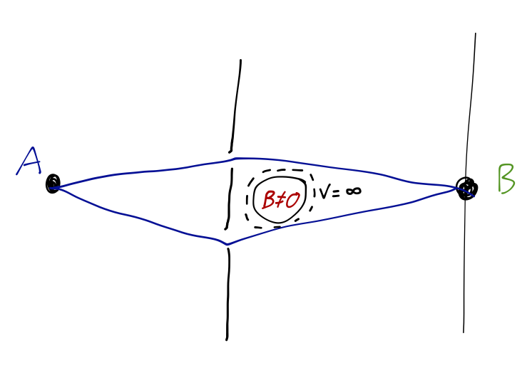
Let’s see what happens. Following our previous notation, we’ll take \vec{x}_1 to be a point at the source S, and \vec{x}_N to be a point somewhere in the interference or detection region, I. To apply path integration, we need the classical Lagrangian to start with; similar to the Hamiltonian, it is derived by insisting that the classical equations of motion give us the Lorentz force law back. The general result is: \mathcal{L} = \frac{1}{2} m \dot{\vec{x}}^2 - q \Phi(x) + \frac{q}{c} \dot{\vec{x}} \cdot \vec{A}. Here we just want to look at a magnetic effect, so we set the scalar potential \Phi(x) = 0. We’re mainly interested in the change in the action induced by the final term when the vector potential is switched on. Along a particular path segment from (\vec{x}_{n-1}, t_{n-1}) to (\vec{x}_n, t_n), we have S = \int_{t_{n-1}}^{t_n} dt\ \mathcal{L} = S_0 + \int_{t_{n-1}}^{t_n} dt\ \frac{q}{c} \dot{\vec{x}} \cdot \vec{A} \\ = S_0 + \frac{q}{c} \int_{\vec{x}_{n-1}}^{\vec{x}_n} \vec{A} \cdot \vec{ds}. Thus, if we combine all of the infinitesimal paths together along our particle’s trajectory, we just end up with the sum of all of these infinitesimal line integrals, which is equal to the total line integral over the path: e^{iS/\hbar} = e^{iS_0 / \hbar} \exp \left[ \frac{iq}{\hbar c} \int_{\vec{x}_1}^{\vec{x}_N} \vec{A} \cdot \vec{ds} \right]. This expression gives us the phase shift for one particular path, so now we have to carry out the sum over all possible paths. Fortunately, this is easier than it seems. As we just recalled above, the line integral of \vec{A} around any closed path is equal to the magnetic flux contained inside, \oint \vec{A} \cdot \vec{ds} = \Phi_{B, \textrm{int}}. Of course, if we take any path from S to I, and combine it with a path back from I to S, we have a closed path. Thus, if we combine two paths which both pass above or below the solenoid, the enclosed flux is zero, and we find \left[\int_S^I \vec{A} \cdot \vec{ds} + \int_I^S \vec{A} \cdot \vec{ds'}\right]_{\textrm{above}} = \left[\int_S^I \vec{A} \cdot \vec{ds} + \int_I^S \vec{A} \cdot \vec{ds'}\right]_{\textrm{below}} = 0 However, if we take one path above and one below, then the impenetrable cylinder is enclosed, and we have a non-zero difference, \left[ \left( \frac{q}{\hbar c}\right) \int_{\vec{x}_1}^{\vec{x}_N} \vec{A} \cdot \vec{ds} \right]_{\textrm{above}} - \left[ \left( \frac{q}{\hbar c}\right) \int_{\vec{x}_1}^{\vec{x}_N} \vec{A} \cdot \vec{ds} \right]_{\textrm{below}} = \frac{q \Phi_B}{\hbar c}. Note that this tells us something important, namely that even though the magnetic field \vec{B} is identically zero everywhere outside the cylinder, the vector potential \vec{A} is not zero. The specific choice of vector potential is gauge-dependent, but one possibility is \vec{A} = \frac{Br_0^2}{2r} \hat{\phi} where r_0 is the radius of the cylinder, and we’ve taken it to be oriented along the z-axis at the origin.
The contribution to the probability of observation at point \vec{x}_N (and thus the beam intensity) goes as the modulus squared of the amplitude, i.e. for two paths P_1 and P_2 we have I \supset \left| \int [dx]_{P_1} e^{iS/\hbar} \right|^2 + \left| \int [dx]_{P_2} e^{iS/\hbar} \right|^2 + 2 \textrm{Re} \left[ \int [dx]_{P_1} e^{iS/\hbar} \int [dx]_{P_2} e^{-iS/\hbar} \right]. (where the symbol \supset means “contains”, since these are a few terms out of many contributing to I.) The B-dependent differences between paths always cancel out in the absolute-value squared terms, but in the interference term, if P_1 and P_2 together circle around the solenoid, they contribute a phase difference of the form e^{iq\Phi_B / \hbar c}, and so in the final intensity we find oscillating dependence on the magnetic flux, I \supset \cos \frac{q \Phi_B}{\hbar c}. Once again, the effect of the magnetic field is observable despite the fact that the cylinder is impenetrable, and the particle never experiences a Lorentz force due to the field! As with the other interference experiments, this is also a purely quantum-mechanical effect, with the oscillations becoming infinitely rapid (and thus unobservable) as \hbar \rightarrow 0.
The Aharonov-Bohm experiment (which has been carried out and verified in the laboratory) once again leads us to the conclusion that \vec{A}, and not \vec{B}, is the more “fundamental” object in quantum mechanics!
The conclusion we draw from Aharonov-Bohm seems almost contradictory: the vector potential \vec{A} is “real”, and yet somehow it’s also not unique - we can modify it by an arbitrary gauge transformation without changing the physics. (People sometimes describe this as an “infinite redundancy” in our physical description, since an infinite family of gauge fields give the same result.) But philosophically, this really isn’t that different from the simpler “infinite redundancy” that we’re all already used to, which is that V(x) and V(x) + V_0 both give the same physics as well.
For ordinary potentials, we can restate this slightly: physical answers resulting from V(x) only depend on potential differences, which are always “gauge-invariant” since the choice of V_0 cancels out. Similarly, although the “reality” of the \vec{A} field is essential to the Aharonov-Bohm effect, the answer depends not on the gauge-dependent \vec{A} but on the gauge-invariant magnetic flux. Like the shift V_0 in the scalar potential, the gauge-dependent parts of \vec{A} have to cancel out in physical observables.
26.5 Charge quantization
At this point, we can make a connection to group theory again, which will lead us to an interesting physical consequence. As I’ve emphasized above, we can think of the electromagnetic interactions as arising fundamentally from the presence of the local gauge invariance of the wavefunction under transformations of the form \psi(x,t) \rightarrow e^{i\theta(x)} \psi(x,t). This is a symmetry; we’re requiring that our theory be invariant under such transformations. It is a local or gauge symmetry because the symmetry operations can be different at every point in space. But what is the symmetry group? Clearly this is a continuous symmetry, since \theta(x) is continuous; it’s also obviously a group since if we apply two gauge transformations, it’s equivalent to a single combined transformation since e^{i\alpha(x)} e^{i\beta(x)} = e^{i(\alpha(x) + \beta(x))}, and we obviously have an inverse and identity, etc. As for what group this is, there are actually two options:
- The group is U(1), the Lie group of “one by one unitary matrices”, i.e. complex numbers z that satisfy |z| = 1. The group operation is multiplication, and the group elements are unique up to factors of 2\pi, i.e. \alpha and \alpha + 2\pi are the same group element.
- The group is \mathbb{R}, the group of real numbers. The group operation is addition, and \alpha is a different group element from \alpha + 2\pi.
In either case, the gauge transformation rule holds as above, with \psi(x,t) transforming as a one-dimensional representation of either U(1) or \mathbb{R}. In the U(1) case this is the defining representation - the natural way that we write the definition of the group. It’s easy to verify that this also gives a good representation of \mathbb{R} (albeit not faithful, since \rho(\alpha) and \rho(\alpha + 2n\pi) map to the same complex number, but this is okay.) For most practical purposes, there isn’t much distinction between U(1) or \mathbb{R} - they act in the same way to just give pure-phase gauge transformations to our wavefunction.
However, there is one important and subtle way in which the two gauge groups actually differ. We know that the charge of our particle matters: as a simple example, we know that a neutron (which is neutral) shouldn’t transform at all. From our derivation above, the transformation of the wavefunction for a particle of charge Q is \psi(x,t) \rightarrow e^{iQ \theta(x)} \psi(x,t). In more mathematical language, every choice of charge Q determines a distinct representation of the gauge group: for a given group element \alpha, \rho_Q(\alpha) = e^{iQ\alpha}. This seemingly gives us an infinite number of representations, since Q can be any real number; if the gauge group is \mathbb{R}, then this observation is true. However, if the group is U(1), there is actually a constraint on Q from the fact that \alpha and \alpha + 2\pi are the same element of the group. Since representations can’t map the same group element to different objects, we see that \rho_Q(\alpha + 2\pi) = \rho_Q(\alpha) \\ e^{iQ(\alpha + 2\pi)} = e^{iQ\alpha} \\ \Rightarrow e^{2\pi i Q} = 1 which tells us that Q must be an integer! This is only true if the gauge group is U(1); if it is \mathbb{R}, then shifting by 2\pi gives a different group element and so there is no such condition.
Now, you might object that the charge of the electron is not an integer, which is certainly true - it is also dimensionful. But the fundamental unit of charge is hiding inside of \theta(x), since we recall from our derivation above that \theta(x) = q \Lambda(x) / \hbar c. This fixes the units; what we’ve actually proved is that for U(1), the charge is quantized, i.e. all charges are an integer multiple of the fundamental charge e.
This is, in fact, what we observe in nature, although it’s hard to definitively say that there is no object anywhere in the Universe with charge that isn’t just a unit of e. (There are some fairly good experimental constraints based on looking for fractionally charged objects getting stuck in sea water or other materials.) Actually, there is a small asterisk on this statement: in the Standard Model of particle physics, the smallest electric charge is carried by the up quark, with q_u = +1/3 e. So the real “unit charge” is 1/3 of the electron’s charge! The story is complicated by the fact that quarks feel the strong nuclear force which binds them so strongly that they are “confined” - i.e. it’s impossible to observe a free up quark. None of this contradicts U(1) charge quantization - it just changes what the unit is.
26.5.1 Magnetic monopoles
There is one other very interesting corollary of the choice of gauge group, which is the existence of magnetic monopoles. To see how magnetic monopoles are related to the choice of U(1) or \mathbb{R} as the electromagnetic gauge group, we need to understand what the consequences are of having a magnetic monopole in a quantum system.
As you know, Maxwell’s laws are for the most part very symmetric between the \vec{E} and \vec{B} fields, particularly once special relativity is taken into account. The electric charge density sources the divergence of the electric field, \nabla \cdot \vec{E} = 4\pi \rho. Similarly, a hypothetical magnetic charge (i.e. a magnetic monopole) would source a magnetic field with a divergence, \nabla \cdot \vec{B} = 4\pi \rho_M. Suppose that such a monopole existed, with magnetic charge e_M. Placing it at the origin of our coordinates, we obtain a static magnetic field \vec{B} = \frac{e_M}{r^2} \hat{r}. To consider the quantum mechanics of this system, we need to find the vector potential \vec{A} that gives rise to this magnetic field. In spherical coordinates, the \hat{r} component of the curl is given by \nabla \times \vec{A} = \hat{r} \left[ \frac{1}{r \sin \theta} \frac{\partial}{\partial \theta} (A_\phi \sin \theta) - \frac{\partial A_{\theta}}{\partial \phi} \right] + ... By inspection, the following vector potential looks like it will work: \vec{A} = \left[ \frac{e_M (1 - \cos \theta)}{r \sin \theta} \right] \hat{\phi}. (I’m not writing out the other components of the curl, but rest assured they vanish as needed.) This gives the correct \vec{B} field, but it has a problem; we see that along the negative \hat{z} axis, \sin \theta = 0 but \cos \theta = -1, and the vector potential is infinite! In fact, it’s not too hard to prove that any single function \vec{A} will have a singularity somewhere in order to generate the given magnetic field.
One way out is to use a pair of vector potentials, and stitch them together somehow. Let’s define \begin{cases} \vec{A}^{(I)} = \left[ \frac{e_M(1-\cos \theta)}{r \sin \theta} \right] \hat{\phi}, & \theta < \pi-\epsilon; \\ \vec{A}^{(II)} = -\left[ \frac{e_M(1+\cos \theta)}{r \sin \theta} \right] \hat{\phi}, & \theta > \epsilon. \end{cases} These two potentials are good almost everywhere, except the negative and positive \hat{z} axis respectively; by using them both together, we can obtain the correct magnetic field everywhere. Since they do give the same magnetic field, we know that where the two vector potentials overlap, they must be related by a gauge transformation. The difference between the potentials is very simple: \vec{A}^{(II)} - \vec{A}^{(I)} = - \left( \frac{2e_M}{r \sin \theta} \right) \hat{\phi}. The \hat{\phi} component of the gradient in spherical coordinates is \nabla \Lambda = \hat{\phi} \frac{1}{r \sin \theta} \frac{\partial \Lambda}{\partial \phi} + ... so the gauge transformation is very simple, \Lambda = -2e_M \phi. Now we get to the interesting part. If we consider the quantum mechanical motion of a particle with charge e in the field generated by the magnetic monopole, then we know that the vector potential is significant, and in particular the wavefunctions corresponding to the use of \vec{A}^{(I)} or \vec{A}^{(II)} are related to each other by a phase, \psi^{(II)} = e^{ie \Lambda/\hbar c} \psi^{(I)} = \exp \left( \frac{-2ie e_M \phi}{\hbar c}\right) \psi^{(I)}. The wavefunction has to be single-valued, which means that it is unique at each point in space; so if we’re using angular coordinates, we must find that going around by, say, 2\pi in the polar angle \phi returns us to our starting point. This must be independently true for both \psi^{(I)} and \psi^{(II)}. If we consider the wavefunctions on the equator, then going around from \phi=0 to \phi=2\pi must give us the same value for both wavefunctions, which means by the equation above we must have \frac{2 e e_M}{\hbar c} = \pm n for some integer n. This is not some abstract argument about symmetries: this comes from an actual rotation in space, so this physical condition must be satisfied!
The quantization of the product of charges lets us connect back to our statements about gauge symmetries above. If the gauge group is U(1), then electric charge is quantized; if electric charge is quantized, then so is magnetic charge, in units of e_M \sim \frac{\hbar c}{2|e|}. On the other hand, if the gauge group is \mathbb{R}, then since e can take on any value, so can e_M. But then doing the experiment for fixed e_M and different e would lead us to a contradiction - so we conclude that without quantized electric charge, magnetic monopoles cannot exist! Observation of a magnetic monopole would definitively prove that the real world is described by a U(1) gauge interaction, and not by \mathbb{R}.
There are deeper and more mathematically sophisticated ways to prove that magnetic monopoles are forbidden if the gauge group is \mathbb{R}, but allowed for U(1). (None of this formalism proves that monopoles exist at all, but if they do exist, they allow a definitive test for U(1) vs. \mathbb{R}.) If you have a strong math background, you can try to read more about it in this set of advanced lecture notes from Matt Reece. The notes get very deep into particle physics, but the arguments about charge quantization and magnetic monopoles are contained within part one of the notes.