23 Variational methods
Perturbation theory as we’ve introduced it is a very powerful technique; we’ve only seen a handful of examples, and there are many more. However, one of its main limitations is the reliance on starting with a Hamiltonian \hat{H}_0 which we can solve exactly. There are a limited number of such exactly solvable systems in quantum mechanics. What can we do if we’re interested in studying a Hamiltonian for which we can’t start with exact solutions? The variational method offers us a way forward, even if we have no exact solutions. In fact, all we need is a guess at a solution to get started.
23.1 Variational method for ground-state energy
Suppose we are given a Hamiltonian \hat{H} which we have no idea how to solve, but we are able to come up with a “trial” ground state, which we call \ket{\tilde{0}}. We can certainly ask what the expectation value of the energy is in this state: \tilde{E}_0 = \bra{\tilde{0}} \hat{H} \ket{\tilde{0}}. Whatever \ket{\tilde{0}} happens to be, we know that we can use completeness to write it as a sum over energy eigenstates, which I’ll label as \ket{n} with \ket{0} the true ground state: \ket{\tilde{0}} = \sum_{n=0}^{\infty} \ket{n} \left\langle n | \tilde{0} \right\rangle = \sum_{n=0}^\infty c_n \ket{n}. This lets us write out the expectation value as \tilde{E}_0 = |c_0|^2 E_0 + \sum_{n>0} |c_n|^2 E_n. I’ve split the sum up in a suggestive way. Now we make the observation that by definition, the ground-state energy is the lowest energy in the system, which means that \tilde{E}_0 \geq |c_0|^2 E_0 + \sum_{n > 0} |c_n|^2 E_0 = \left( \sum_{n} |c_n|^2 \right) E_0 \\ = \left\langle \tilde{0} | \tilde{0} \right\rangle E_0. In other words, assuming we normalize our trial state \ket{\tilde{0}}, then the trial energy is always greater than or equal to the ground-state energy, E_0 \leq \frac{\bra{\tilde{0}} \hat{H} \ket{\tilde{0}}}{\left\langle \tilde{0} | \tilde{0} \right\rangle}. (We carry around the normalization factor \left\langle \tilde{0} | \tilde{0} \right\rangle mainly as a reminder to ourselves that we’re just working with guesses here, and they need not be properly normalized states. You can just normalize your trial wavefunctions and not bother carrying it around, it’s up to you.)
There are two important observations to make based on these results. First of all, we see that for absolutely any choice of trial wavefunction, the energy \tilde{E}_0 is an upper bound on the true ground-state energy. So even if we choose trial wavefunctions completely at random, we will still gain some information about the system.
The second important observation is that if we have two different trial wavefunctions, then whichever one has lower energy is typically a better approximation of the true ground state. This is obvious from the equations above; lower energy generally means that the overlap of the trial wavefunction with the ground state |c_0| must be larger, at the expense of the other |c_n|s. (This isn’t completely rigorous, just because we can also change the energy by shuffling around overlap with higher states while leaving |c_0| fixed. But lower energy states tend to have better overlap with the ground state.) The converse statement is a bit stronger: as \tilde{E}_0 \rightarrow E_0 we must have |c_0| \rightarrow 1.
Rather than guessing completely at random, it’s much more efficient to define a family of trial wavefunctions that depend on some adjustable parameters, \ket{\tilde{0}(\alpha_1, \alpha_2, ...)}. We can then “search” through the space of all of these functions to find the best one, i.e. the minimum-energy solution: we calculate \tilde{E}_0(\alpha_1, \alpha_2, ...) = \bra{\tilde{0}(\alpha_1, \alpha_2, ...)} \hat{H} \ket{\tilde{0}(\alpha_1, \alpha_2, ...)} and then solve for the parameters \alpha such that \frac{\partial \tilde{E}_0}{\partial \alpha_i} = 0. If there are multiple solutions (as there often will be), we can simply compare the energies directly to find the global minimum-energy trial wavefunction. This approach is known as the variational method.
In the above derivation, I isolated a single ground state. A good question is, what happens if the ground state has a degeneracy so it is no longer unique?
First of all, it should be noted that nothing in the derivation of the bound on \tilde{E}_0 assumed that the other energy eigenstates were not degenerate with the ground state; we just used that E_n \geq E_0, which is still true if any number of the E_n are equal to E_0. So the basic result doesn’t care about the presence of degeneracy.
However, there is one important difference that shows up in the presence of degeneracy, which is what happens to the trial state as the bound is saturated. To understand that, let’s explicitly consider a case with a doubly-degenerate ground state, spanned by two kets \ket{0} and \ket{0'}. Then we have \ket{\tilde{0}} = c_0 \ket{0} + c_0' \ket{0'} + \sum_{n=1}^\infty c_n \ket{n} and the resulting trial-state energy is \tilde{E}_0 = |c_0|^2 E_0 + |c_0'|^2 E_0 + \sum_{n=1}^\infty |c_n|^2 E_n.
Now as the bound approaches the true value, \tilde{E}_0 \rightarrow E_0, we have |c_0|^2 + |c_0'|^2 \rightarrow 1 which means that all other |c_n| \rightarrow 0. So now the trial state becomes a linear combination of the degenerate states, \ket{\tilde{0}} \rightarrow c_0 \ket{0} + c_0' \ket{0'}.
There is now a family of trial states that all saturate the bound and all have the same energy. This means that if we perform a variational calculation by introducing some parameters, then there will be a flat direction - a ray in parameter space where we can change the state without changing the energy. We will see this in our variational analysis, as long as our parameter space happens to contain the true ground state(s); there may be some remnant of this flat direction in the more general case, but it’s hard to say anything definite in general.
The variational method is much more flexible than perturbation theory. It requires no small parameters, and no exact solutions, just a Hamiltonian and a trial state. It is used very commonly in physics research, and played a crucial role in understanding of superconductivity and the fractional quantum Hall effect, among many other applications. All of that being said, the variational method suffers from one significant weakness; we have no way to determine how close we are to the true ground state. The bounds we obtain are rigorous, but even if we try millions of trial wavefunctions, we have no way to tell from the variational bound alone whether our best energy is within 0.1% or 1000% of the true ground-state energy.
Despite its drawbacks, it is usually the case that the variational method tends to give quite good results for the ground-state energy in particular, even if we pick a fairly bad trial wavefunction. It’s straightforward to “prove” why this is the case. Suppose we guess the correct ground state up to a small mixture of an excited state, \ket{\tilde{0}} = \ket{0} + \epsilon \ket{1}. (taking \epsilon real for simplicity.) The resulting energy estimate would be E_0 \leq \frac{\bra{\tilde{0}} \hat{H} \ket{\tilde{0}}}{\left\langle \tilde{0} | \tilde{0} \right\rangle} = \frac{E_0 + \epsilon^2 E_1}{1 + \epsilon^2} = E_0 + \mathcal{O}(\epsilon^2). So even a significant 10% error in the state vector (\epsilon = 0.1) gives just a 1% error in the ground-state energy. This is a consequence of the fact that the Hamiltonian operator is diagonal in the energy eigenstates, which causes any terms linear in \epsilon to vanish.
This explains why variational estimates can often be much better than you might expect! The main downside in practical applications is that we typically don’t have any way to estimate what \epsilon is reliably.
As mentioned above, as we reduce our variational bound, the trial state becomes a closer approximation of the true ground state. This does mean that we can use the trial wavefunction to estimate other expectation values as well. However, if we do there’s no good way to tell how wrong the answer is, since the rigorous bound we’re relying on only applies to the ground-state energy, not to other observables. We can also see immediately that we generally expect such estimates for other observables to be worse: we have \bra{\tilde{0}} \hat{O} \ket{\tilde{0}} = \bra{0} \hat{O} \ket{0} + \epsilon (\bra{0} \hat{O} \ket{1} + \bra{1} \hat{O} \ket{0}) + ... which fails to match the expectation value of \hat{O} in the true ground state at order \epsilon, rather than \epsilon^2.
Let’s do a couple of examples to see how this works in practice.
23.1.1 Example: the harmonic oscillator
Let’s start with the simple harmonic oscillator, \hat{H} = \frac{\hat{p}^2}{2m} + \frac{1}{2} m \omega^2 \hat{x}^2. Suppose that we had no idea how to solve for the eigenstates here, but we had a feeling that the quadratic potential should give us a wavefunction which is symmetric and somewhat localized near x=0. We might take a simple Gaussian as our trial wavefunction: \tilde{\psi}(x) = \left(\frac{\beta}{\pi}\right)^{1/4} e^{-\beta x^2/2}, where we’ve taken a single parameter \beta. Now we calculate the trial energy: \tilde{E}(\beta) = \sqrt{\frac{\beta}{\pi}} \int_{-\infty}^\infty dx\ e^{-\beta x^2/2} \left[ -\frac{\hbar^2}{2m} \frac{\partial^2}{\partial x^2} + \frac{1}{2} m \omega^2 x^2 \right] e^{-\beta x^2/2} \\ = \sqrt{\frac{\beta}{\pi}} \int_{-\infty}^\infty dx\ \left[ -\frac{\hbar^2 }{2m} \left( -\beta + \beta^2 x^2 \right) + \frac{1}{2} m \omega^2 x^2\right] e^{-\beta x^2}. Now we have to remember our formula for a Gaussian integral: \int_{-\infty}^\infty dx\ e^{-\beta x^2} = \sqrt{\frac{\pi}{\beta}}, which means that \int_{-\infty}^\infty dx\ x^2 e^{-\beta x^2} = -\frac{\partial}{\partial \beta} \left( \sqrt{\frac{\pi}{\beta}}\right) \\ = \frac{1}{2\beta} \sqrt{\frac{\pi}{\beta}}. Plugging back in above, \tilde{E}(\beta) = \frac{\hbar^2 \beta}{2m} + \frac{1}{2\beta} \left( -\frac{\hbar^2 \beta^2}{2m} + \frac{1}{2} m \omega^2 \right) \\ = \frac{\hbar^2 \beta}{4m} + \frac{m \omega^2}{4\beta}. Now we minimize: \frac{d\tilde{E}}{d\beta} = \frac{\hbar^2}{4m} - \frac{m\omega^2}{4\beta^2} = 0 from which we see that the optimum value is \beta = \frac{m\omega}{\hbar}, and the corresponding energy is \tilde{E}_{\textrm{min}} = \frac{1}{2} \hbar \omega. This is exactly the ground-state energy, and of course we’ve recovered the exact ground-state wavefunction as well. If we happen to guess a class of functions which contains the true ground-state, then that’s what the variational procedure will return. (Sakurai goes through a similar example for the hydrogen atom.)
23.1.2 Example: particle in a box
Let’s try the one-dimensional particle in a box next, V(x) = \begin{cases} 0, & |x| < a; \\ \infty, & |x| > a, \end{cases} The exact ground-state solutions are, to remind ourselves, \left\langle x | 0 \right\rangle = \frac{1}{\sqrt{a}} \cos \left( \frac{\pi x}{2a} \right), \\ E_0 = \frac{\pi^2 \hbar^2}{8ma^2}. The only constraint on the trial state \ket{\tilde{0}} is that we must be able to write it as a linear combination of true energy eigenstates, which means that it has to satisfy any relevant boundary conditions; in this case, we can only use trial wavefunctions which satisfy \tilde{\psi}(\pm a) = 0.
This time, let’s intentionally pick a trial wavefunction that doesn’t map onto one of the exact solutions, taking a polynomial instead of trig functions. The simplest such function we can write down which vanishes at both boundaries is a parabola, \left\langle x | \tilde{0} \right\rangle = a^2 - x^2. This is a zero-parameter trial function, but let’s see how well it reproduces the ground-state energy as a guess. It’s also obviously not normalized (it has the wrong dimensions), so we have to make sure to divide out by the normalization. Doing so, we have \tilde{E}_0 = \frac{\bra{\tilde{0}} \hat{H} \ket{\tilde{0}}}{\left\langle \tilde{0} | \tilde{0} \right\rangle} \\ = \frac{ \left( -\frac{\hbar^2}{2m}\right) \int_{-a}^a (a^2 - x^2) \frac{d^2}{dx^2} (a^2 - x^2) dx}{\int_{-a}^a (a^2 - x^2)^2 dx} \\ = \left(\frac{10}{\pi^2}\right) \left( \frac{\pi^2 \hbar^2}{8ma^2} \right), factoring out the ground-state energy. The correction factor actually turns out to be surprisingly small: \tilde{E}_0 = \frac{10}{\pi^2} E_0 \approx 1.0132 E_0. So our most naive guess gives the correct ground-state energy to almost within 1%! We can do even better if we actually include a parameter to vary over; let’s try the family of trial wavefunctions \tilde{\psi}(x) = \left\langle x | \tilde{0} \right\rangle = |a|^\lambda - |x|^\lambda. with \lambda as our variational parameter, restricted to \lambda > \tfrac{1}{2}.
Calculate the trial energy \tilde{E}_0(\lambda) for the wavefunction \tilde{\psi}(x) given above.
Answer:
Let’s compute the normalization first. The absolute value is necessary since we have rational exponents on a and x, but we can get rid of it in the integrals by just using symmetry and restricting to positive x:
\left\langle \tilde{0} | \tilde{0} \right\rangle = \int_{-a}^a dx |\tilde{\psi}(x)|^2 \\ = 2\int_0^a dx (a^\lambda - x^\lambda)^2 \\ = \frac{4\lambda^2}{(1+\lambda)(1+2\lambda)} a^{2\lambda+1}.
Moving on to the numerator, \bra{\tilde{0}} \hat{H} \ket{\tilde{0}} = -\frac{\hbar^2}{2m} \int_{-a}^a dx (a^\lambda - x^\lambda) \frac{d^2}{dx^2} (a^\lambda - x^\lambda) \\ = +\frac{\hbar^2}{m} \int_0^a dx (a^\lambda - x^\lambda) \lambda(\lambda-1) x^{\lambda-2} \\ = \frac{\hbar^2}{m} \lambda(\lambda-1) \frac{\lambda}{(\lambda-1)(2\lambda-1)} a^{2\lambda-1}.
(Note that if we didn’t impose \lambda > 1/2 there would be some issues here!) Dividing through, some factors cancel and we’re left with
\tilde{E}_0 = \frac{\hbar^2}{4ma^2} \frac{\lambda^2}{2\lambda-1} \frac{(1+\lambda)(1+2\lambda)}{\lambda^2} \\ = \left[ \frac{(\lambda+1)(2\lambda+1)}{(2\lambda-1)} \right] \frac{\hbar^2}{4ma^2}.
From the exercise above, you should recover the answer \tilde{E}_0(\lambda) = \left[ \frac{(\lambda+1)(2\lambda+1)}{(2\lambda-1)} \right] \frac{\hbar^2}{4ma^2}. Since this gives an upper bound on the true ground-state energy E_0 for any value of \lambda, we differentiate and find the minimum \tilde{E}_0, which then gives us our “best guess” for the true ground-state energy and wavefunction. Here, the minimizing value is \lambda = \frac{1+\sqrt{6}}{2} \sim 1.72, and the resulting ground-state energy is \tilde{E}_{min} = \left( \frac{5+2\sqrt{6}}{\pi^2} \right) E_0 \approx 1.00298 E_0. Not bad for such a simple guess!
In this case, since we have access to the true solution we can also evaluate how well the wavefunction itself imitates the true ground state. The direct approach would be simply to calculate \left\langle 0 | \tilde{0} \right\rangle, but we can also derive a bound in a similar way to our bound on the energy. Expanding in a complete set of states, we see that \tilde{E}_{min} = \sum_{k=0}^{\infty} |\left\langle k | \tilde{0} \right\rangle|^2 E_k \\ \geq |\left\langle 0 | \tilde{0} \right\rangle|^2 E_0 + 9E_0 (1-|\left\langle 0 | \tilde{0} \right\rangle|^2), where 9E_0 is the energy of the first parity-even excited state. We’re just keeping the first two terms in the sum; if \ket{\tilde{0}} overlaps with higher states, the contribution will be larger. If we invert this and solve for the overlap, we find that |\left\langle 0 | \tilde{0} \right\rangle|^2 \geq 0.99963, a very significant overlap; if we interpret this as an angle between two vectors, i.e. |\left\langle 0 | \tilde{0} \right\rangle| = \cos \theta, then the corresponding angle is approximately 1 degree.
Here, you should complete Tutorial 11 on “Variational method”. (Tutorials are not included with these lecture notes; if you’re in the class, you will find them on Canvas.)
23.2 Variational method for excited states
It is also possible to use the variational method to obtain estimates for excited states as well, but the procedure is much more delicate. If we have a trial ket for the first excited state, for example, we can write \ket{\tilde{1}} = \sum_{n=0}^{\infty} d_n \ket{n} and then \tilde{E}_1 = |d_0|^2 E_0 + |d_1|^2 E_1 + \sum_{n>1} |d_n|^2 E_n. At this point we’re stuck, unless we are able to guarantee that the trial excited state has no overlap with the true ground state, i.e. d_0 = 0. If this is the case, then the inequality we want immediately follows, E_1 \leq \frac{\bra{\tilde{1}} \hat{H} \ket{\tilde{1}}}{\left\langle \tilde{1} | \tilde{1} \right\rangle}, with the trial estimate approaching the true state \ket{1} as the energy decreases.
Unfortunately, this is very difficult to do in practice; usually if we know the exact ground state \ket{0}, we don’t need to use the variational method. We can certainly construct a trial excited state \ket{\tilde{1}} which is orthogonal to the trial ground state \ket{\tilde{0}}, but then the inequalities are no longer guaranteed, and without some other input there’s no way for us to be sure our estimates aren’t very poor.
The main exception is when a symmetry is present. If we are interested in an excited state that has different conserved quantum numbers from the ground state, then we can once again find a rigorous upper limit without worrying about orthogonality (because the symmetry guarantees orthogonality for us, basically.)
The canonical example is, again, the hydrogen atom. A variational estimate of the 2p energy level can be carried out with rigor, because the 2p level is the lowest level with orbital angular momentum l=1; as long as we take our trial wavefunction to include Y_1^m(\theta, \phi), orthogonality to the lower-energy s states is automatic. On the other hand, the 2s energy level would be much more difficult to access if we didn’t know the exact form of the hydrogen solutions. (But we could keep going up to 3d, 4f, and so on with variational estimates!)
Let’s do a simple example anyway, going back to the square well. The square-well Hamiltonian as written above has parity as a good symmetry, \hat{P} \hat{H} \hat{P} = \hat{H}, which means that its energy eigenfunctions are either even or odd under parity. In this case, since we have the exact solutions available, we know that the ground state (and our previous trial wavefunction) are both parity-even. Let’s see what happens if we try a parity-odd trial wavefunction: \left\langle x | \tilde{1} \right\rangle = x (a^2 - x^2). A straightforward integration (there’s nothing to vary here) yields the energy estimate \tilde{E}_1 = \frac{\bra{\tilde{1}} \hat{H} \ket{\tilde{1}}}{\left\langle \tilde{1} | \tilde{1} \right\rangle} = 1.0639 E_1, fairly close to the first excited state energy (although not quite as good as the ground state estimate.) We could certainly do better if we introduced some variational parameters.
To summarize: the variational method can be used for excited states, but only easily and rigorously if we’re looking for the lowest excited state with some symmetry property that the ground state doesn’t have. Otherwise, the best we can do is try to obtain a good ground-state estimate and then carefully construct a variational state which is orthogonal to it (but this isn’t fully under our control, unfortunately.) The basic idea to remember is thus: the variational method gives reliable estimates for the lowest energy eigenvalue in each available symmetry channel.
23.3 The Rayleigh-Ritz variational method
So far, our approach has been to write a single trial wavefunction with some parametric dependence, and then calculate the trial energy and minimize with respect to those parameters. For the simple examples we’ve done above, this is fine, but for more complicated systems trying to carry out the variation with a single function quickly becomes unwieldy. For one thing, the dependence on the parameters can often be non-linear, as in our square-well example where our trial function was \left\langle x | \tilde{0} \right\rangle = |a|^\lambda - |x|^\lambda. As the number of parameters increases, trying to minimize a complicated non-linear function can become a difficult task. Another problem with having a single trial wavefunction is that if you want to improve your estimate, there’s no systematic way to add more variational parameters.
For these reasons, in practical research applications a slight modification known as the Rayleigh-Ritz or linear variational method is widely used. Instead of starting with a single trial wavefunction, we choose a trial basis of N states \{\ket{j}\} and let the trial state be a linear combination: \ket{\tilde{0}} = \sum_{j=1}^N c_j \ket{j}. (Here I assume the trial basis is orthonormal, which is usually a good idea and makes things simpler; in practice one can do Rayleigh-Ritz with a non-orthonormal trial basis too.) To make life easier, we insist that the c_j are chosen to give the normalization \left\langle \tilde{0} | \tilde{0} \right\rangle = 1 for the trial state, i.e. \left\langle \tilde{0} | \tilde{0} \right\rangle = 1 = \sum_{k=1}^N \sum_{j=1}^N c_k^\star c_j Then the trial ground-state energy is \tilde{E}_0 = \bra{\tilde{0}} \hat{H} \ket{\tilde{0}} \\ = \sum_{j=1}^N \sum_{k=1}^N c_k^\star c_j \bra{k} \hat{H} \ket{j}. Now we have a variational problem in the N linear coefficients c_j. However, we can’t just take the derivative with respect to c_j of this last expression and solve, because we want to keep the normalization condition too. We can instead use the method of Lagrange multipliers, by adding the constraint times a parameter E to the unconstrained function: \frac{\partial}{\partial c_i^\star} \left[ \bra{\tilde{0}} \hat{H} \ket{\tilde{0}} - E (\left\langle \tilde{0} | \tilde{0} \right\rangle - 1)\right] = 0, or plugging in the expansions, \frac{\partial}{\partial c_i^\star} \left[ \sum_{jk} c_k^\star \hat{H}_{kj} c_j - E \sum_m c_m^\star c_m \right] = 0, giving the set of linear equations \sum_j (\hat{H}_{ij} c_j - \delta_{ij} E c_j) = 0. This is nothing more than the eigenvalue-eigenvector equation for \hat{H} in the trial basis! The value of the lowest-energy solution \tilde{E}_0 to this equation gives us our best variational upper bound on the true ground-state energy. In fact, we could have skipped to this result at the beginning: if we start by diagonalizing \hat{H} in the trial space, obtaining trial energy eigenstates \{\ket{\tilde{E}_j}\}, then we could have written \ket{\tilde{0}} = \sum_{j=1}^N c_j' \ket{\tilde{E}_j} and obviously the “best” trial wavefunction is given by choosing c_j' = 1 for the lowest-energy trial eigenstate, and 0 for the rest.
Another advantage of the Rayleigh-Ritz approach is apparent here, which is that it gives us immediate estimates for all of the excited states as well; diagonalizing \hat{H} over the trial basis automatically gives us a set of N kets which are mutually orthogonal, and so the variational bounds apply to each one in turn (although only the ground-state bound will be rigorous as we have discussed above).
Finally, I’ll note that the Rayleigh-Ritz approach makes it easy in principle to improve our variational estimate, just by adding more states to the trial basis; our bounds can only improve with more states. If we have to re-diagonalize the entire, enlarged matrix then this doesn’t save us any work, but there are a number of standard algebraic techniques that let us quickly re-diagonalize if we have already diagonalized part of the full Hamiltonian matrix.
Unfortunately, there isn’t really a good example for us to do on the board; the Rayleigh-Ritz method mainly lends itself to the use of computers, since it’s most effective when we can use a large basis. I’ll at least set up a common example for you, which is the anharmonic oscillator: \hat{H} = \frac{\hat{p}^2}{2m} + \frac{1}{2} m \omega^2 \hat{x}^2 + \lambda \hat{x}^4. Perturbation theory can allow us to make some progress here, but no matter how small \lambda is the perturbative solution will always break down for the higher excited states. However, the Rayleigh-Ritz variational method is quite effective here. The unperturbed harmonic oscillator states \ket{n} give us a natural choice of trial basis, up to some chosen maximum n. Working in that basis, we can rewrite \hat{x}^4 \propto (\hat{a} + \hat{a}^\dagger)^4 This gives us an extremely nice-looking Hamiltonian as a matrix in the trial basis. In particular, the Hamiltonian is band diagonal; the \hat{x}^4 term only connects state \ket{n} to states between \ket{n-4} and \ket{n+4}, and all other matrix elements further from the diagonal are guaranteed to be zero. Diagonalizing the Hamiltonian in some finite basis is thus relatively easy. Here’s what I get if I carry this procedure out as a function of the number of basis states N used, setting \lambda = 0.1 and all other physical quantities to 1 for simplicity:
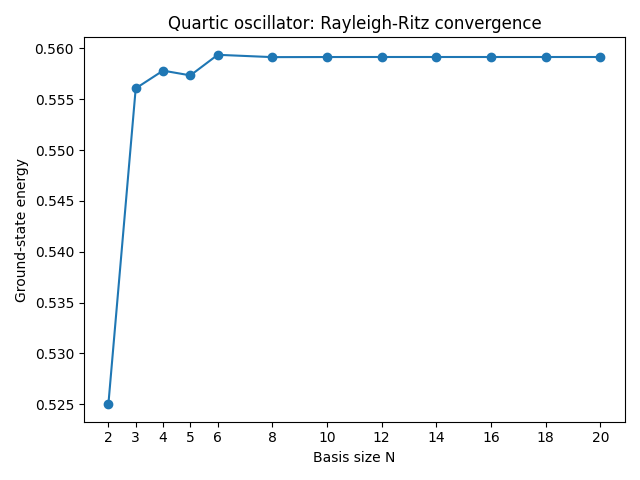
We can compare the Rayleigh-Ritz results for this simple case to numerical solutions to the full Schrodinger equation, and the variational method actually works extremely well; the convergence to the true solutions is found to be exponential in the size of the trial basis, even if \lambda is large! (You can see just from the simple example above that the convergence to a consistent result looks pretty exponential, although this doesn’t establish how close it is to the true answer.) This is an example of a system where the variational method is extremely powerful. In fact, proofs of convergence to the true solutions sometimes exist for Rayleigh-Ritz; the variational method can be rigorous after all!
23.4 Positivity bounds
Much earlier in these notes (and probably long before you took this class), we encountered another type of inequality in quantum mechanics in the form of uncertainty relations (Section 3.4), the most famous of which was the Heisenberg uncertainty principle, \Delta x \Delta p \geq \hbar/2.
This is a lower bound on expectation values of operators, as opposed to the upper bounds we get from variational estimates. Can we find a way to combine both approaches to bracket an energy estimate and know how far off we are?
Although we derived the more general uncertainty relation using Cauchy-Schwarz and some other definitions, there is another, much simpler lens through which we can obtain the uncertainty relation, the idea of positivity. The starting point is the observation that if we have any operator \hat{A} (not necessarily Hermitian!), then we immediately have the bound \bra{\psi}\hat{A}^\dagger \hat{A} \ket{\psi} \geq 0 for any state \ket{\psi}. This is often written simply as \left\langle \hat{A}^\dagger \hat{A} \right\rangle \geq 0. It’s very easy to see this has to be true: if \hat{A} \ket{\psi} = \ket{\chi}, then this is just the statement that \left\langle \chi | \chi \right\rangle \geq 0. (There are some “reasonable” assumptions on the Hilbert space and the operator if we want to be careful about the math.)
The positivity bound is a surprisingly powerful statement because it has to hold for any operator that we build. For example, consider the operator \hat{A} \equiv \hat{x} + i \alpha \hat{p}. Notice that we’ve included an arbitrary parameter \alpha, which I’ll assume is real. Positivity from this operator then implies the result: \left\langle (\hat{x} - i\alpha \hat{p})(\hat{x} + i\alpha\hat{p}) \right\rangle \geq 0 \\ \left\langle \hat{x}^2 \right\rangle + \alpha^2 \left\langle \hat{p}^2 \right\rangle + i \alpha \left\langle \hat{x} \hat{p} - \hat{p} \hat{x} \right\rangle \geq 0 \\ \left\langle \hat{x}^2 \right\rangle + \alpha^2 \left\langle \hat{p}^2 \right\rangle - \hbar \alpha \geq 0 using [\hat{x}, \hat{p}] = i\hbar. Now, the quadratic formula lets us factorize the left-hand side, (\alpha - \alpha_+) (\alpha - \alpha_-) \geq 0, where the roots are \alpha_\pm = \frac{1}{\left\langle 2\hat{p}^2 \right\rangle} \left[ \hbar \pm \sqrt{\hbar^2 - 4 \left\langle \hat{x}^2 \right\rangle \left\langle \hat{p}^2 \right\rangle} \right]. The only way that the inequality above can be true for all \alpha is if the roots \alpha_{\pm} are both complex (or equal), which means the argument under the square root has to be negative (or zero), so we can read off the result: \left\langle \hat{x}^2 \right\rangle \left\langle \hat{p}^2 \right\rangle \geq \frac{\hbar^2}{4}. This is the Heisenberg uncertainty principle! (Assuming that \left\langle \hat{x} \right\rangle = \left\langle \hat{p} \right\rangle = 0, but in systems where that isn’t necessarily true we can easily generalize the proof above to show the uncertainty principle for \Delta x and \Delta p.)
We can get more physics out of the same operator. Consider the simple harmonic oscillator \hat{H} = \frac{\hat{p}^2}{2m} + \frac{1}{2} m \omega^2 \hat{x}^2 = \frac{1}{2} m \omega^2 \left( \hat{x}^2 + \frac{1}{m^2 \omega^2} \hat{p}^2 \right) Setting \alpha = 1/(m \omega) above, we read off the bound \left\langle \hat{x}^2 \right\rangle + \frac{1}{m^2 \omega^2} \left\langle \hat{p}^2 \right\rangle \geq \frac{\hbar}{m \omega} But now this combination of operators is just the Hamiltonian up to a constant, so we find \left\langle \hat{H} \right\rangle \geq \frac{\hbar \omega}{2} \Rightarrow E_0 \geq \frac{\hbar \omega}{2} since E_0 is an expectation value of \hat{H} in the ground state. Since we have the advantage of knowing the true solution, we know that in fact the ground-state energy saturates this bound (it becomes an equality.)
This simple example shows us a path to a more general approach to ground-state energies: by combining variational estimates with positivity constraints, we can always obtain a bracket on the true ground-state energy, E_0^{\rm pos} \leq E_0 \leq E_0^{\rm var}.
As with going from the basic variational method to Rayleigh-Ritz, a more sophisticated approach to positivity constraints uses as many operators as possible, with each giving its own inequality, and then tries to combine all of the resulting bounds to obtain a better result. The calculational method used to obtain a joint result from a set of inequalities goes under the name of semi-definite programming (and doing semi-definite programming to apply positivity bounds is also known by the name “quantum bootstrap”.) This is taking us close to the forefront of how people study quantum systems, and I won’t say more about it here, but you now know the basic idea and enough terminology to go find more results if you’re interested.