20 Time-independent perturbation theory
There are a very limited number of quantum-mechanical systems which we can solve analytically from start to finish; to deal with realistic systems, we usually have to resort to some sort of approximation. We’ve seen one such method already, the WKB approximation. However useful WKB is, it can only be applied under fairly special conditions. The general idea of perturbation theory, in which we systematically expand our solutions in some available small parameter, is much more general.
The basic idea of perturbation theory should be familiar to you already - at its core, it just boils down to series expansion in a small parameter. But there are some important subtleties specific to quantum mechanics, especially once time dependence enters in. We’ll start with “time-independent” perturbation theory.
20.1 Rayleigh-Schrödinger perturbation theory
The setup here is very simple: we assume that we are interested in a system described by a Hamiltonian \hat{H} = \hat{H}_0 + \lambda \hat{W}, where \lambda is some small, continuous parameter. We assume that in the \lambda \rightarrow 0 limit, we have a full analytic solution to the system described by \hat{H}_0, i.e. we have solved the eigenvalue problem \hat{H}_0 \ket{n^{(0)}} = E_n^{(0)} \ket{n^{(0)}}. Our new task is to find the eigenvalues and eigenstates of the full Hamiltonian, (\hat{H}_0 + \lambda \hat{W}) \ket{n} = E_n \ket{n}.
We haven’t said anything about what \lambda is, exactly; the nature of \lambda depends strongly on what problem we’re trying to solve. Most commonly, \lambda is a natural expansion parameter, some small dimensionless number which appears in the full Hamiltonian; for example, the fine-structure constant \alpha = e^2 / (\hbar c) \approx 1/137 is an excellent expansion parameter if we’re studying corrections due to electromagnetic effects.
Sometimes, \lambda isn’t even anything physical at all: it can be used as an auxiliary variable, where we take an existing \hat{W}, multiply by arbitrary \lambda, do the expansion and set \lambda = 1 at the end. On the other extreme, \lambda can even be a real tunable parameter, like the strength of an electric field in your experimental apparatus.
To proceed, we search for a power-series solution in \lambda for both the eigenenergies and eigenstates of the full Hamiltonian: \ket{n} = \ket{n^{(0)}} + \lambda \ket{n^{(1)}} + \lambda^2 \ket{n^{(2)}} + ... \\ E_n = E_n^{(0)} + \lambda E_n^{(1)} + \lambda^2 E_n^{(2)} + ... We can take these expansions and simply plug back into the (time-independent) Schrödinger equation: (\hat{H}_0 + \lambda \hat{W}) \left( \ket{n^{(0)}} + \lambda \ket{n^{(1)}} + \lambda^2 \ket{n^{(2)}} + ...\right) \\ = \left( E_n^{(0)} + \lambda E_n^{(1)} + \lambda^2 E_n^{(2)} + ... \right) \left( \ket{n^{(0)}} + \lambda \ket{n^{(1)}} + \lambda^2 \ket{n^{(2)}} + ... \right) Now we simply proceed order by order. At order \lambda^0, we recover the \hat{H}_0 eigenvalue equation in full. First order is more interesting: we find (\hat{H}_0 - E_n^{(0)}) \ket{n^{(1)}} = (E_n^{(1)} - \hat{W}) \ket{n^{(0)}} and continuing to second order, (\hat{H}_0 - E_n^{(0)}) \ket{n^{(2)}} = (E_n^{(1)} - \hat{W}) \ket{n^{(1)}} + E_n^{(2)} \ket{n^{(0)}}. Clearly we can keep going as far as we want, although things start to get messy beyond second order; in cases where you need to go to high order, Brillouin-Wigner perturbation theory (to be described below) is a better choice to set things up.
20.1.1 First-order energy eigenvalues and eigenstates
For now, we assume that all of the eigenvalues E_n^{(0)} of \hat{H}_0 are non-degenerate; we’ll come back to deal with that complication later. We also assume that we’re dealing with a discrete system (although if n becomes a continuous label instead, all the derivations are very similar, replacing sums with integrals as appropriate.)
Now, notice that if we multiply by the zeroth-order eigenstate on the left side, we have \bra{n^{(0)}} (\hat{H}_0 - E_n^{(0)}) \ket{n^{(1)}} = 0, letting \hat{H}_0 act to the left. Therefore, we see that \bra{n^{(0)}} (E_n^{(1)} - \hat{W}) \ket{n^{(0)}} = 0, i.e. the zeroth-order energy has been shifted by the amount \Delta_n^{(1)} = \lambda E_n^{(1)} = \bra{n^{(0)}} \lambda \hat{W} \ket{n^{(0)}}. This proves the result we have borrowed before, namely that the first-order energy shift in perturbation theory is simply the expectation value of the perturbation with respect to the old eigenstates. Intuitively, it makes sense that we don’t need the first-order states \ket{n^{(1)}} for this: the effect of \hat{W} on the eigenstates themselves begins at order \lambda, and so corrections in expectation values due to the states shifting will only appear starting at second order.
Now let’s find the eigenstates. Since we presumably know what all of the zeroth-order eigenstates are, a reasonable approach would be to try and expand \ket{n^{(1)}} in terms of the states \ket{m^{(0)}}: \ket{n^{(1)}} = \sum_{m \neq n} c_m \ket{m^{(0)}}. Note that we explicitly exclude the state \ket{n^{(0)}} from the sum, i.e. we take \left\langle n^{(1)} | n^{(0)} \right\rangle = 0. Fixing the normalization of our states \left\langle n | n \right\rangle = 1 leads to this condition as a requirement; we can also notice that from the first-order equation above, we can add an arbitrary amount of \ket{n^{(0)}} to \ket{n^{(1)}} without affecting the equation.
Show that the condition of normalizing the states \left\langle n | n \right\rangle = 1 is automatically satisfied at first order if we have \left\langle n^{(1)} | n^{(0)} \right\rangle = 0.
Answer:
Just taking the expansion of \ket{n} defined above and plugging it in to \left\langle n | n \right\rangle, we start organizing terms order by order in \lambda: \left\langle n | n \right\rangle = \left\langle n^{(0)} | n^{(0)} \right\rangle + \lambda \left[\left\langle n^{(1)} | n^{(0)} \right\rangle + \left\langle n^{(0)} | n^{(1)} \right\rangle \right] \\ + \lambda^2 \left[ \left\langle n^{(0)} | n^{(2)} \right\rangle + \left\langle n^{(1)} | n^{(1)} \right\rangle + \left\langle n^{(2)} | n^{(0)} \right\rangle \right] + ... If we want to have properly normalized states both before and after perturbation, i.e. \left\langle n | n \right\rangle = \left\langle n^{(0)} | n^{(0)} \right\rangle = 1, then all of the correction terms have to vanish identically, i.e. \sum_{k=0}^j \left\langle n^{(j-k)} | n^{(k)} \right\rangle = 0 from order \lambda^j in the expansion above. So things get more complicated at second order (where the condition relates \left\langle n^{(0)} | n^{(2)} \right\rangle to -\left\langle n^{(1)} | n^{(1)} \right\rangle.) Note that we could also alternatively impose that \left\langle n^{(0)} | n^{(1)} \right\rangle is pure imaginary to automatically satisfy the first-order constraint.
Although we can impose this normalization condition on the states as we go, it’s not vital that we do so; in fact, in a later section below we’re going to choose a completely different condition that makes the state \ket{n} improperly normalized. There is nothing wrong with using unnormalized states: when we come to calculating probabilities or expectation values, we can always just “renormalize” the state by dividing out the norm, \ket{\psi}_N = \frac{1}{\left\langle \psi | \psi \right\rangle} \ket{\psi}.
Going back to our first-order equation and using this expansion gives \sum_{m \neq n} (\hat{H}_0 - E_n^{(0)}) c_m \ket{m^{(0)}} = (E_n^{(1)} - \hat{W}) \ket{n^{(0)}} \\ \sum_{m \neq n} (E_m^{(0)} - E_n^{(0)}) c_m \ket{m^{(0)}} = (E_n^{(1)} - \hat{W}) \ket{n^{(0)}}. If we multiply on the left by another arbitrary eigenstate \ket{k^{(0)}}, we can collapse the sum: \sum_{m \neq n} \bra{k^{(0)}} c_m (E_k^{(0)} - E_n^{(0)}) \ket{m^{(0)}} = E_n^{(1)} \delta_{kn} - \bra{k^{(0)}} \hat{W} \ket{n^{(0)}} Setting k=n makes the left side vanish, and just returns our expression for E_n^{(1)}. If instead we require k \neq n, then the E_n^{(1)} term vanishes, the sum on the left collapses, and we end up with the expression c_k = \frac{\bra{k^{(0)}} \hat{W} \ket{n^{(0)}}}{E_n^{(0)} - E_k^{(0)}} and so \ket{n^{(1)}} = \sum_{k \neq n} \ket{k^{(0)}} \frac{W_{kn}}{E_n^{(0)} - E_k^{(0)}}. where I’ve introduced a more compact notation for the matrix elements of \hat{W} with respect to the unperturbed basis, W_{kn} = \bra{k^{(0)}} \hat{W} \ket{n^{(0)}}. Don’t forget that the order matters, in general; W_{nk} = W_{kn}^\star, so flipping the order of the indices comes with a complex conjugation. (Typically \hat{W} will be Hermitian since it’s part of a Hamiltonian, in which case this doesn’t matter.)
It’s easy to remember that the sum above is only over k \neq n; if you try to include that term, it will blow up! Similarly, if any of the energy eigenvalues are degenerate, the sum also blows up, so you can see why we had to make that assumption in deriving this. (If there is such a degeneracy, then the derivation above gives us no information on the corresponding c_k, so we’ll have to find another approach.)
20.1.2 Going to second order in energy
In general, the eigenstates at order n-1 are all we need to compute the energies at order n. We won’t keep going indefinitely, but now that we’ve found the first-order eigenstates, it’s easy enough to continue and get the energy corrections at second order. Returning to our above equation for the second-order perturbation and again dotting in \ket{n^{(0)}} on the left, we see that E_n^{(2)} = \bra{n^{(0)}} (\hat{W} - E_n^{(1)}) \ket{n^{(1)}}. The second term is zero since as we argued above, \ket{n^{(0)}} and \ket{n^{(1)}} are orthogonal. Expanding the first term out, E_n^{(2)} = \bra{n^{(0)}} \hat{W} \left( \sum_{k \neq n} \ket{k^{(0)}} \frac{\bra{k^{(0)}} \hat{W} \ket{n^{(0)}}}{E_n^{(0)} - E_k^{(0)}} \right) \\ = \sum_{k \neq n} \frac{|W_{nk}|^2}{E_n^{(0)} - E_k^{(0)}}.
An easy way to remember the sign of the denominator in the second-order correction is to remember the fact that the correction to the ground-state energy n=0 is always negative. This is not simply a coincidence; if we look at the expectation value of the full Hamiltonian with respect to the zeroth-order eigenstates, we see \bra{n^{(0)}} \hat{H} \ket{n^{(0)}} = \sum_{m} \left\langle n^{(0)} | m \right\rangle \bra{m} \hat{H} \ket{m} \left\langle m | n^{(0)} \right\rangle, where \ket{m} are the eigenstates of the full Hamiltonian. But that means that the matrix elements are just the true energy values of \hat{H}: \bra{n^{(0)}} \hat{H} \ket{n^{(0)}} = \sum_m E_m |\left\langle n^{(0)} | m \right\rangle|^2. The squared inner products under the sum are exactly the probabilities for observing zeroth-order eigenstate \ket{n^{(0)}} in full eigenstate \ket{m}; the sum over all of them will be 1, in particular. Meanwhile, the left-hand side is just the first-order energy, i.e. E_n^{(0)} + \lambda \bra{n^{(0)}} \hat{W} \ket{n^{(0)}} = \sum_m E_m |\left\langle n^{(0)} | m \right\rangle|^2. Since the first-order energy eigenvalues are given by a weighted sum over the full energy eigenvalues, with positive weights, we conclude that the distribution of all the approximate energy eigenvalues must be more closely spaced than that of the true eigenvalues. This explains is why the next correction is negative for the ground-state; it tends to increase the overall spread in all energy eigenvalues as the true solution is approached.
Let’s collect our results together and summarize:
Given a Hamiltonian of the form \hat{H} = \hat{H}_0 + \hat{W}, in terms of the energy eigenvalues \ket{E_n^{(0)}} of \hat{H}_0, the corrected energy to second order in perturbation theory is given by E_n = E_n^{(0)} + \lambda W_{nn} + \lambda^2 \sum_{k \neq n} \frac{|W_{nk}|^2}{E_n^{(0)} - E_k^{(0)}} + ... while the first-order corrected energy eigenstates are \ket{n} = \ket{n^{(0)}} + \sum_{k \neq n} \frac{\lambda W_{kn}}{E_n^{(0)} - E_k^{(0)}} \ket{k^{(0)}} + ...
The sign of the total second-order energy correction is always negative for the ground state.
20.2 Controlled example: the harmonic oscillator
The best way to test out a new method is of course to apply it to a system where you already know the answer. So let’s take the one-dimensional harmonic oscillator, and add a “perturbation” to it of the same quadratic form: \hat{H} = \frac{\hat{p}{}^2}{2m} + \frac{1}{2} m\omega^2 \hat{x}^2 + \lambda \hat{x}^2. Of course, we don’t need perturbation theory to deal with this: for any value of \lambda, we can just rewrite this as W(\hat{x}) = \frac{1}{2} m (\omega^2 + \frac{2\lambda}{m}) \hat{x}^2 = \frac{1}{2} m \omega'{}^2 \hat{x}^2 where \omega' = \sqrt{\omega^2 + \frac{2\lambda}{m}} \approx \omega + \frac{\lambda}{m \omega} - \frac{\lambda^2}{2m^2 \omega^3} + ... Note that \lambda has the same units as m \omega^2, which is a quick check that our expansion is sensible.
Now, we go back and identify \hat{H}_0 = \frac{\hat{p}{}^2}{2m} + \frac{1}{2} m\omega^2 \hat{x}^2, \\ \lambda \hat{W} = \lambda \hat{x}^2 The unperturbed (zeroth-order) energies are then E_{n}^{(0)} = \hbar \omega \left(n + \frac{1}{2} \right), corresponding to the standard eigenstates \ket{n^{(0)}}. The first-order energy correction is then E_n^{(1)} = \bra{n^{(0)}} \hat{x}{}^2 \ket{n^{(0)}}. We can work this out using the ladder operators: E_n^{(1)} = \frac{\hbar}{2m\omega} \bra{n^{(0)}} (\hat{a} + \hat{a}^{\dagger})^2 \ket{n^{(0)}} \\ = \frac{\hbar}{2m\omega} \bra{n^{(0)}} (\hat{a} \hat{a}^{\dagger} + \hat{a}^\dagger \hat{a}) \ket{n^{(0)}} \\ = \frac{\hbar}{m\omega} (n+\frac{1}{2}). (Note that this is valid since we know how \hat{a} acts on eigenstates of \hat{H}_0, even though the ladder operators don’t commute with the perturbation itself. A big advantage of perturbation theory is being able to use our existing methods to deal with \hat{H}_0!) Plugging this back in above, we find that E_n \approx E_n^{(0)} + \lambda E_n^{(1)} = \hbar \left( \omega + \frac{\lambda}{m \omega} \right) \left(n + \frac{1}{2}\right), matching our first-order expansion of \omega' above.
Note that we’re using the ladder operators constructed explicitly for the unperturbed Hamiltonian \hat{H}_0 here. There’s nothing inconsistent about this approach, since they were defined explicitly from a rearrangement of the simple harmonic oscillator Hamiltonian, \hat{H}_0. In general, when we add a perturbation we will simply find that \hat{N} = \hat{a}^\dagger \hat{a} defined in this way will still commute with \hat{H}_0, but not with the full \hat{H}. In our current example, it’s easy to see that \hat{a}^\dagger \hat{a} = \frac{\hat{H}_0}{\hbar \omega} - \frac{1}{2} \\ \Rightarrow \hat{H} = \hbar \omega (\hat{N} + \frac{1}{2}) + \lambda \hat{x}^2 and [\hat{N}, \hat{x}^2] = \frac{\hbar}{2m\omega}[\hat{N}, (\hat{a} + \hat{a}^{\dagger})^2] \\ = \frac{\hbar}{2m\omega} \left( [\hat{N}, \hat{a} + \hat{a}^\dagger] (\hat{a} + \hat{a}^\dagger) + (\hat{a} + \hat{a}^\dagger) [\hat{N}, \hat{a} + \hat{a}^\dagger) \right) \\ = \frac{\hbar}{2m\omega} \left( (-\hat{a} + \hat{a}^\dagger) (\hat{a} + \hat{a}^\dagger) + (\hat{a} + \hat{a}^\dagger) (-\hat{a} + \hat{a}^\dagger) \right) \\ = \frac{\hbar}{m\omega} \left( \hat{a}^\dagger \hat{a}^\dagger - \hat{a} \hat{a} \right) which is clearly not zero. In this special case, we can of course define new ladder operators \hat{a}' which use the modified frequency \omega', and then everything will commute and we can label the states of the full Hamiltonian with the new number operator \hat{N}'. However, this is only because we can map the perturbative problem back onto the full SHO here. Normally, when we deal with perturbations, we want to work in terms of the operators and states of the analytically solvable \hat{H}_0 only.
Let’s keep going, and look at the second-order energy shift. To evaluate it, we will need the matrix elements of \hat{W} between arbitrary zeroth-order energy eigenstates. We already evaluated the diagonal case, now we need the explicitly off-diagonal terms k \neq n: \bra{k^{(0)}} \hat{W} \ket{n^{(0)}} = \frac{\hbar}{2m\omega} \bra{k^{(0)}} \hat{a}{}^2 + (\hat{a}^\dagger)^2 \ket{n^{(0)}} \\ = \frac{\hbar}{2m\omega} \left[ \sqrt{n(n-1)} \delta_{k,n-2} + \sqrt{(n+1)(n+2)} \delta_{k,n+2} \right] So the sum over all states for the second-order energy correction collapses: E_n^{(2)} = \sum_{k \neq n} \frac{|W_{nk}|^2}{E_n^{(0)} - E_k^{(0)}} \\ = \frac{\hbar^2}{4m^2 \omega^2} \left[ \frac{n(n-1)}{\hbar \omega (n - (n-2))} + \frac{(n+1)(n+2)}{\hbar \omega (n-(n+2))}\right] \\ = \frac{\hbar}{8m^2 \omega^3} \left[ n(n-1) - (n+1)(n+2) \right] \\ = \frac{-\hbar}{2m^2 \omega^3} \left(n + \frac{1}{2} \right). Multiplying by \lambda^2, we see that our second-order formula becomes E_n \approx E_n^{(0)} + \lambda E_n^{(1)} + \lambda^2 E_n^{(2)} \\ = \hbar \left( \omega + \frac{\lambda}{m \omega} - \frac{\lambda^2}{2m^2 \omega^3} \right) \left(n + \frac{1}{2} \right), again nicely matching our series expansion of the exact solution.
20.2.1 Another controlled example: the shifted harmonic oscillator
We could use the formula we derived above to solve for the eigenstates at first order as well; but since the position wavefunction of the harmonic oscillator doesn’t have a simple dependence on the parameter \omega, it would be a rather complicated exercise. Instead, let’s turn to another form of perturbed simple harmonic oscillator: V(\hat{x}) = \frac{1}{2} m \omega^2 \hat{x}^2 + \lambda L \hat{x}. so \hat{W} = L \hat{x}, and I’ve introduced a distance scale L just so that \lambda has the same units as above. Notice that once again, we can turn this into an ordinary SHO with a change of variables: completing the square, the potential above is equal to V(\hat{x}) = \frac{1}{2} m \omega^2 \left( \hat{x} + \frac{\lambda}{m \omega^2} L \right)^2 - \frac{\lambda^2 L^2}{2m \omega^2} This rewritten harmonic oscillator has the same frequency \omega, but its position has been translated by -\lambda L / (m \omega^2), and the overall energy has been shifted by -\lambda^2 L^2 / (2m\omega^2). The energy levels of the SHO don’t depend on where the origin is, so the energy shift is exactly proportional to \lambda^2 and independent of n: \Delta E_n = -\frac{\lambda^2 L^2}{2m \omega^2}. This means that if we attempt to calculate the perturbation at first order, we should find zero, and indeed we see immediately that E_n^{(1)} = \sqrt{\frac{\hbar}{2m\omega}} \bra{n^{(0)}} (\hat{a} + \hat{a}^\dagger) \ket{n^{(0)}} = 0 for all n.
Extend the energy eigenvalue calculation to second order in perturbation theory for this system, and show that you recover the expected result.
Answer:
Proceeding to second order, the off-diagonal matrix elements are
\bra{k^{(0)}} \hat{W} \ket{n^{(0)}} = \sqrt{\frac{\hbar}{2m\omega}} L \bra{k^{(0)}} (\hat{a} + \hat{a}^\dagger) \ket{n^{(0)}} \\ = \sqrt{\frac{\hbar}{2m\omega}} L (\sqrt{n} \delta_{k,n-1} + \sqrt{n+1} \delta_{k,n+1}).
so \lambda^2 E_n^{(2)} = \sum_{k \neq n} \frac{|W_{nk}|^2}{E_n^{(0)} - E_k^{(0)}} \\ = \frac{\hbar \lambda^2 L^2}{2m\omega} \left(\frac{n}{\hbar \omega (n-(n-1))} + \frac{n+1}{\hbar \omega (n-(n+1))} \right) \\ = \frac{\lambda^2 L^2}{2m\omega^2} (n-(n+1)) = -\frac{\lambda^2 L^2}{2m\omega^2} independent of n as expected.Now let’s look at the energy eigenstates themselves; since our perturbation can be rewritten as a translation, we expect a relatively simple change to the energy eigenstate wavefunctions. Let’s focus on the ground state \ket{0} explicitly. First applying the formula for the first-order eigenket, we have \ket{0^{(1)}} = \sum_{k \neq n} \ket{k^{(0)}} \frac{W_{kn}}{-\hbar \omega k} \\ = -\ket{1^{(0)}} \frac{L}{\omega} \sqrt{\frac{1}{2m\hbar\omega}} so the corrected ground state at first order is \ket{0} \approx \ket{0^{(0)}} + \lambda \ket{0^{(1)}} = \ket{0^{(0)}} - \frac{\lambda L}{\omega} \sqrt{\frac{1}{2m\hbar \omega}} \ket{1^{(0)}}. Does this match what we expect? Since we’re shifting the harmonic oscillator, the easiest way to compare is using the position-space wavefunctions. We have for the unperturbed wavefunctions \left\langle x | 0^{(0)} \right\rangle = \left(\frac{m \omega}{\pi \hbar}\right)^{1/4} \exp \left[ -\frac{m\omega}{2\hbar} {x}^2 \right], \\ \left\langle x | 1^{(0)} \right\rangle = \left(\frac{m \omega}{\pi \hbar}\right)^{1/4} \sqrt{\frac{2m\omega}{\hbar}} x \exp \left[ -\frac{m\omega}{2\hbar} {x}^2 \right]. Putting this back together, then, the first-order corrected ground state wavefunction is \left\langle x | 0 \right\rangle \approx \left(\frac{m \omega}{\pi \hbar}\right)^{1/4} \left(1 - \frac{\lambda L}{\omega} \sqrt{\frac{1}{2m\hbar \omega}} \sqrt{\frac{2m\omega}{\hbar}} x \right) \exp \left[ -\frac{m \omega}{2\hbar} x^2 \right] \\ = \left(\frac{m \omega}{\pi \hbar}\right)^{1/4} \left(1 - \frac{\lambda L x}{\hbar \omega} \right) \exp \left[ -\frac{m \omega}{2\hbar} x^2 \right] which is precisely what we get if we take \left\langle x | 0^{(0)} \right\rangle, shift x \rightarrow x + (\lambda / m \omega^2) L, and then series expand to first order in \lambda, confirming our result.
Now that we’ve had some practice, let’s move on to a more formal treatment of perturbation theory.
20.3 Formal solution and Brillouin-Wigner perturbation theory
Let’s revisit our starting point and try to write our expansion in a slightly more formal way, to make continuing to higher orders look more systematic. Going back to the beginning, the eigenvalue equation that we’re trying to solve can be written in the form (\hat{H}_0 - E_n) \ket{n} = -\lambda \hat{W} \ket{n}. To derive the formulas we’ve been using, we plugged in power-series expansions for both E_n and \ket{n} and then organized order by order in \lambda. But we can try to reorganize slightly first, by rewriting this as: (E_n^{(0)} - \hat{H}_0) \ket{n} = (\lambda \hat{W} - \Delta_n) \ket{n}, where we’ve defined \Delta_n \equiv E_n - E_n^{(0)}, which is the energy shift due to the perturbation. Now, if we can find an inverse to the operator on the left-hand side, we can rewrite this formally to give us a solution: \ket{n} = (E_n^{(0)} - \hat{H}_0)^{-1} (\lambda \hat{W} - \Delta_n) \ket{n}. There is one problem with this as written, even assuming all of the energy states are non-degenerate: for the specific state \ket{n^{(0)}}, the operator (E_n^{(0)} - \hat{H}_0) gives zero and so its inverse isn’t well-defined. To fix this, we just have to treat \ket{n^{(0)}} specially. First, we define the complementary projection operator to state \ket{n^{(0)}}: \hat{\phi}_n \equiv 1 - \ket{n^{(0)}}\bra{n^{(0)}} = \sum_{k \neq n} \ket{k^{(0)}}\bra{k^{(0)}}.
In general, the notation above where we write a fraction involving two operators is ambiguous, because the order of operators matters. In this case, we are free to adopt the fraction notation since the projection operator can be applied on either side of the inverse of E_n^{(0)} - \hat{H}_0: \frac{1}{E_n^{(0)} - \hat{H}_0} \hat{\phi}_n = \hat{\phi}_n \frac{1}{E_n^{(0)} - \hat{H}_0} = \hat{\phi}_n \frac{1}{E_n^{(0)} - \hat{H}_0} \hat{\phi}_n.
The combination of this operator with the inverse above is always (with no degeneracy in the energies) well-defined, so we combine them to define a new operator: \hat{R}_n \equiv \frac{1}{E_n^{(0)} - \hat{H}_0} \hat{\phi}_n = \sum_{k \neq n} \frac{1}{E_n^{(0)} - E_k^{(0)}} \ket{k^{(0)}} \bra{k^{(0)}}. This projects out the problematic state and leaves us with something well-defined. Finally, we have to put one piece back: we know that in the limit \lambda \rightarrow 0 we should have \ket{n} = \ket{n^{(0)}}, so we should write our general solution as \ket{n} = \ket{n^{(0)}} + \hat{R}_n (\lambda \hat{W} - \Delta_n) \ket{n}. Here I’ve imposed a different state normalization known as intermediate normalization, which sets \left\langle n^{(0)} | n \right\rangle = 1. This is “intermediate” since the states \ket{n} themselves are no longer properly normalized; we’ll deal with this below. But before we worry about that, let’s appreciate how nice this formal rewriting is! Although the unknown corrected state \ket{n} appears on both sides of this equation (so it is an implicit solution), this form gives us a obvious path to iterative solution. Plugging in \ket{n} = \ket{n^{(0)}} on the right-hand side immediately gives us the first-order corrected state, \ket{n} \approx \ket{n^{(0)}} + \hat{R}_n (\lambda \hat{W} - \Delta_n) \ket{n^{(0)}}, from which we can read off \ket{n^{(1)}} = \lambda \hat{R}_n \hat{W} \ket{n^{(0)}} = \sum_{k \neq n} \ket{k^{(0)}} \frac{\bra{k^{(0)}} \lambda \hat{W} \ket{n^{(0)}}}{E_n^{(0)} - E_k^{(0)}} (where the energy term vanishes, even though \Delta_n = \lambda E_n^{(1)} + ..., because \hat{R}_n \ket{n^{(0)}} = 0.) This recovers our expression from before. What about the energy corrections? Going back to the second equation in this section and hitting it with \bra{n^{(0)}} to the left, we have \bra{n^{(0)}} (\lambda \hat{W} - \Delta_n) \ket{n} = 0, so using intermediate normalization, \Delta_n = \bra{n^{(0)}} \lambda \hat{W} \ket{n}.
The first-order energy correction is readily seen to be \bra{n^{(0)}} \lambda \hat{W} \ket{n^{(0)}} as we expect. So we have a very nice setup for iterative solution: we find \ket{n^{(1)}} using the implicit equation above, then use that to find E_n^{(2)}, then plug in the first-order states and energies to find \ket{n^{(2)}}, and so on.
We can keep going, although this is not part of my main lecture notes since the expressions get unwieldy. At second order, we see that E_n^{(2)} = \bra{n^{(0)}} \hat{W} \ket{n^{(1)}} \\ = \bra{n^{(0)}} \hat{W} \frac{\hat{\phi}_n}{E_n^{(0)} - \hat{H}_0} \hat{W} \ket{n^{(0)}} which is easy to see matches the second-order energy formula from above - if this isn’t obvious, plug in the explicit form of the operators above and show it.
Higher order states and energies can be built up in succession just by applying more copies of the projection operator and \hat{W}. In general, we can write the equation for \ket{n} as a power series on both sides: \ket{n^{(1)}} + \lambda \ket{n^{(2)}} + ... = \\ \hat{R}_n (\hat{W} - E_n^{(1)} - \lambda E_n^{(2)} - ...) \times (\ket{n^{(0)}} + \lambda \ket{n^{(1)}} + ...) where I’ve cancelled the zeroth-order terms. Let’s look at the second-order correction, which I avoided doing in our first approach above: \ket{n^{(2)}} = \hat{R}_n \left[ (\hat{W} - E_n^{(1)}) \ket{n^{(1)}} - E_n^{(2)} \ket{n^{(0)}} \right] \\ = \hat{R}_n \hat{W} \hat{R}_n \hat{W} \ket{n^{(0)}} - \hat{R}_n \bra{n^{(0)}} \hat{W} \ket{n^{(0)}} \hat{R}_n \hat{W} \ket{n^{(0)}} where the third term which would arise from E_n^{(2)} vanishes, since it contains the projector \hat{R}_n acting directly on the state \ket{n^{(0)}}. We can keep going to third-order and beyond if needed - the expressions are still messy, but the way we get to them is much more systematic in this operator-based approach.
20.3.1 Wavefunction renormalization
As we have noted, the states \ket{n} derived in this approach are not properly normalized. We can formally “renormalize” the states just by rescaling them: \ket{n}_N = Z_n^{1/2} \ket{n}, where Z_n = 1/\left\langle n | n \right\rangle. Notice that from the equation above, we also have the condition Z_n^{1/2} = \left\langle n^{(0)} | n \right\rangle_N. With the state \ket{n}_N now properly normalized, we can interpret Z_n itself as a probability of finding the perturbed eigenstate \ket{n}_N in the associated unperturbed state \ket{n^{(0)}}. We can clarify this somewhat by expanding in \lambda: Z_n^{-1} = \left\langle n | n \right\rangle = \left\langle n^{(0)} | n^{(0)} \right\rangle + \lambda^2 \left\langle n^{(1)} | n^{(1)} \right\rangle + ... where I’ve once again invoked the fact that \left\langle n^{(0)} | n^{(1)} \right\rangle = 0. Inverting and plugging in the expression for \ket{n^{(1)}} from above, we have Z_n = 1 - \lambda^2 \sum_{k \neq n} \frac{|W_{kn}|^2}{(E_n^{(0)} - E_k^{(0)})^2} + ... The renormalization factor Z_n is less than 1, as it must be since we have a probabilistic interpretation of it. For non-zero \lambda, the probability of observing state \ket{n^{(0)}} is reduced, with the second term representing the sum over probabilities to find any other state as an outcome.
20.3.2 Brillouin-Wigner perturbation theory
There is another way to reorganize our expansion which is can be cleaner in practice, known as Brillouin-Wigner perturbation theory. Building on what we’ve done so far, the formulation is very simple: instead of reorganizing into energy differences before we invert, we just take the very first expression from the derivation above and define an inverse operator: \ket{n} = \ket{n^{(0)}} + \hat{\phi}_n (E_n - \hat{H}_0)^{-1} (\lambda \hat{W}) \ket{n}. (note the sign flip from above.) Defining the combination \hat{Q}_n \equiv \frac{\hat{\phi}_n}{E_n - \hat{H}_0} \hat{W}, we have the simple result \ket{n} = \ket{n^{(0)}} + \lambda \hat{Q}_n \ket{n}. Packaging everything together into a single operator means that writing down the higher-order solutions here are especially simple. In particular, if we plug in the series expansion for \ket{n} in \lambda on both sides, we can just read off \sum_{j} \lambda^j \ket{n^{(j)}} = \ket{n^{(0)}} + \lambda \hat{Q}_n \sum_i \lambda^i \ket{n^{(i)}} \\ \Rightarrow \ket{n^{(j)}} = \hat{Q}_n \ket{n^{(j-1)}} = (\hat{Q}_n)^j \ket{n^{(0)}}, and the corresponding energy correction is, using \Delta_n = \bra{n^{(0)}} \lambda \hat{W} \ket{n} from above, E_n^{(j)} = \bra{n^{(0)}} \hat{W} \ket{n^{(j-1)}} = \bra{n^{(0)}} \hat{W} \hat{Q}_n^{j-1} \ket{n^{(0)}}. These are beautifully simple expressions for the higher-order corrections! The only problem is that if we write out the equations in full, we find that the denominators contain the unknown energy E_n. If we’re solving iteratively and substituting back in to the equations to reach higher orders one at a time, this isn’t a problem; we just plug in E_n at the current order to obtain the next. We could plug in the series for E_n in \lambda and re-expand, but of course that just leads us back to the Rayleigh-Schrödinger picture. The advantage of Brillouin-Wigner is much cleaner expressions, suitable for iteration.
20.4 Example: particle in a warped box
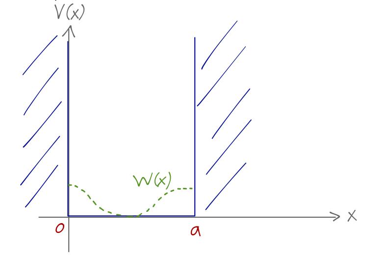
Let’s step back from the formalism and do one more practical example of a calculation before we move on, this time a system where we don’t know the answer in advance. We start with the one-dimensional particle in a box, V(x) = \begin{cases} 0, & 0 \leq x \leq a; \\ \infty, & {\rm elsewhere}. \end{cases} Now we add a perturbation of the form \lambda W(x) = \lambda E' \cos \left( \frac{2\pi x}{a} \right) where now \lambda is dimensionless.
The eigenenergies of the unperturbed system are E_n^{(0)} = \frac{\hbar^2 \pi^2 n^2}{2ma^2} = n^2 E_1^{(0)} and the states can be written simply as \left\langle x | n^{(0)} \right\rangle = \sqrt{\frac{2}{a}} \sin \left( \frac{n\pi x}{a} \right). Let’s evaluate the general matrix elements of \hat{W} with respect to the unperturbed energy eigenstates; since we’re working in position space this will require an integral, W_{mn} = \bra{m^{(0)}} \hat{W} \ket{n^{(0)}} \\ = \frac{2E'}{a} \int_0^a dx\ \sin \left( \frac{m\pi x}{a} \right) \cos \left( \frac{2\pi x}{a} \right) \sin \left( \frac{n \pi x}{a} \right). To evaluate, we can make use of the product-sum formula \sin u \cos v = \frac{1}{2} \left[ \sin (u+v) + \sin (u-v) \right], giving W_{mn} = \frac{E'}{a} \int_0^a dx\ \sin \left( \frac{m \pi x}{a} \right) \left[ \sin \left( \frac{(n+2) \pi x}{a} \right) + \sin \left( \frac{(n-2) \pi x}{a} \right) \right] \\ = \frac{E'}{2} (\delta_{m,n+2} + \delta_{m,n-2}) using the orthogonality of the trig functions on this interval. Actually, this formula is only valid for n > 2; we have to treat n=1 and n=2 separately. It turns out that the product-sum formula actually works for negative values too, but we want to express everything in terms of the states with n>1. For n=2, the second term in the formula goes to \sin ((2-2) \pi x/a) = 0, so we simply have W_{m2} = \frac{E'}{2} \delta_{m, 4}. For n=1, the second term gives instead \sin(-\pi x/a) = - \sin(\pi x/a), and the integration gives W_{m1} = \frac{E'}{2} (\delta_{m,3} - \delta_{m,1}). The first-order energy shifts are given by the diagonal components of this matrix; we see that the only state which overlaps with itself is n=1, and thus E_n^{(1)} = \begin{cases} -E'/2, & n=1; \\ 0, & n>1. \end{cases} The corrected kets at first order are easy to work out as well: \ket{n^{(1)}} = \sum_{k \neq n} \ket{k^{(0)}} \frac{W_{kn}}{E_n^{(0)} - E_k^{(0)}} \\ = \frac{E'}{2E_1} \left[ \frac{\ket{(n-2)^{(0)}}}{n^2 - (n-2)^2} + \frac{\ket{(n+2)^{(0)}}}{n^2 - (n+2)^2} \right] or for the special cases n \leq 2, \ket{2^{(1)}} = -\frac{E'}{24E_1^{(0)}} \ket{4^{(0)}}, \\ \ket{1^{(1)}} = -\frac{E'}{16E_1^{(0)}} \ket{3^{(0)}}. These results make it immediately clear that the figure of merit for whether the dimensionful perturbation E' is small is its ratio to the ground-state energy of the unperturbed box; we should have E_1^{(0)} \gg E' for our expansion to be good.