9 Capstone example: the ammonia maser
Now that we’ve spent a lot of time developing our toolbox, let’s turn to a much more concrete physical example: the ammonia molecule, NH_3. (We’re still going to reduce it to a nice square potential, but at least the starting point is more concrete, and we’ll have to think about modeling.)

The structure of ammonia makes it a particularly interesting case, which is actually simpler than it looks. It is a rather complex molecule, a bound state consisting of a large number of protons, neutrons, and electrons arranged in a complicated way. But part of being a good physicist is knowing what the interesting behavior of a system is, and isolating it.
What are the different possible energy eigenstates of an ammonia molecule? There are many possible ways for it to be put into an excited energy state: it can be moving through space at some speed, or rotating, or the molecular bonds could be vibrating. The electrons, or even the neutrons and protons inside the nuclei, could also be in a higher energy state. Experimentally, we’re able to measure differences between these excited states and the ground state as emission lines, photons which carry away the energy difference.
What spectral lines do we see from ammonia? The shortest-range excitations correspond to the highest energy; exciting the individual electrons requires electron-volts (eV) of energy, corresponding to visible or ultraviolet photons. Nuclear excitations would give gamma rays, in the mega electron-volt (MeV, 10^6 eV) range. Vibration of the molecular bonds has a lower energy, giving infrared photons; rotation of the entire molecule gives far-infrared (milli-electron-volt, meV, or 10^{-3} eV.)
But on top of all that rich structure, there is another set of lines that are even lower energy, giving rise to microwave emissions with a wavelength of about 1 cm (corresponding to energies on the scale of 100 micro-electron volts (\mu eV), or 100 \times 10^{-6} eV.) This doesn’t have the right energy for any of the kinds of energy that we’ve listed so far. In fact, it corresponds to a special kind of motion of the nitrogen relative to the hydrogen atoms, one that is firmly quantum-mechanical.
The pyramid shape of ammonia is fairly rigid, and is a local minimum of the overall potential energy among the four atoms. However, keeping the plane of the three H fixed, it’s obvious that the N can be either above or below the plane with the same energy.

The motion in which the nitrogen switches from above to below the hydrogen plane is known as inversion. Inversion has the lowest energy of all, giving rise to the observed microwave emisisons. Microwave lines are interesting because they are relatively unusual, and the ammonia line is very important in radio astronomy.
This isn’t really a vibrational mode in the normal sense; vibration comes from small deformations around an equilibrium point, but here there is quite a large potential barrier between the two inverted configurations. If we take the N atom to be fixed (since it’s heavy) and let x be the distance from the N to the plane of the hydrogen atoms, then the potential energy V(x) looks something like this:
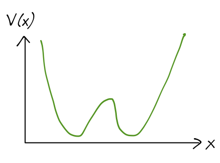
So studying inversion is a one-dimensional problem (now involving the mass of a fictitious particle, the reduced mass 3m_H m_N / (3m_H + m_N).) In fact, we’ll further simplify our model by approximating the true potential with a rectangular one:
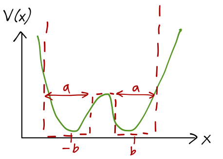
V(x) = \begin{cases} V_0, & |x| \leq b-a/2; \\ 0, & b-a/2 < |x| < b+a/2; \\ \infty, & |x| \geq b+a/2. \end{cases}
This will be good enough to gain a qualitative understanding of the physics. The ground state energy will be some E such that 0 < E < V_0; inversion corresponds to tunneling of the system through the potential barrier.
9.1 Infinite potential barrier
To really understand the tunneling effect, it’s useful to start by taking V_0 \rightarrow \infty as well, so that tunneling is impossible. Then the problem reduces to a double infinite square-well potential. I’ll remind you that the energy eigenvalues for a particle of mass m in an infinite square well of width a are E_n = \frac{\hbar^2 k_n^2}{2m} where k_n = n\pi/a. The boundary conditions are simple: the wavefunction is zero inside the infinite barriers, and so it must vanish at the borders. We can write two possible wavefunctions that aren’t zero everywhere: \psi_L^n(x) = \begin{cases} \sqrt{\frac{2}{a}} \sin \left[ k_n \left(b + a/2 + x\right) \right], & b-a/2 < -x < b+a/2 \\ 0, & {\rm elsewhere}; \end{cases} \\ \psi_R^n(x) = \begin{cases} \sqrt{\frac{2}{a}} \sin \left[ k_n \left(b + a/2 - x\right) \right], & b-a/2 < x < b+a/2 \\ 0, & {\rm elsewhere}; \end{cases} These are just the wavefunctions for the particle being either in the left box or the right box; there is a two-fold degeneracy in the energy eigenvalues, since \psi_1^n(x) and \psi_2^n(x) have the same energy if n is the same.
Even with the infinite potential barrier, there are excited states, and we should expect to find a spectral line for e.g. the n=2 to n=1 transition with frequency (E_2 - E_1) / \hbar. This isn’t what we’re looking for, and in fact is simply a vibrational mode in which the three H atoms move together in small displacement around their equilibrium. Like the other vibrational modes, this gives an infrared emission line.
We can take our localized wavefunctions and recombine them with parity in mind as even and odd wavefunctions \psi_e^n(x) = \frac{1}{\sqrt{2}} [\psi_L^n(x) + \psi_R^n(x)] \\ \psi_o^n(x) = -\frac{1}{\sqrt{2}} [\psi_L^n(x) - \psi_R^n(x)] You can think of this as a sort of “change of basis”: it’s clear that any wavefunction can be expressed either in terms of the individual well eigenstates, or these parity-eigenfunction combinations.
9.2 Finite potential barrier
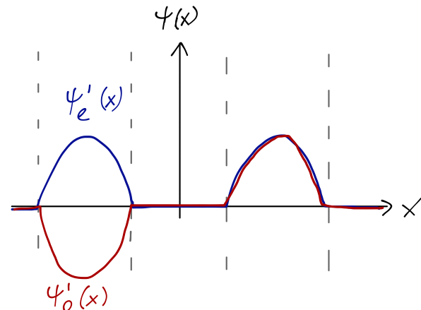
Now we lower the center potential barrier to some finite value V_0, assuming we have E < V_0. The outer barriers are still infinite, so the wavefunction still has to vanish there, which means it takes the general form in the two wells \psi(x) = \begin{cases} A \sin \left[ k (b + a/2 - x) \right],& b-a/2 < x < b+a/2; \\ A' \sin \left[ k (b + a/2 + x) \right],& b-a/2 < -x < b+a/2. \end{cases} Since parity is still a good symmetry of the potential, all possible solutions will divide into the even-parity set A_e = A'_e, and the odd-parity set A_o = -A'_o. There will be a corresponding set of bound-state energies E_e and E_o, with corresponding wave numbers k_e, k_o.
There is now also a non-zero wavefunction inside the central barrier. If we define the usual \kappa = \sqrt{2m(V_0-E)} / \hbar, then the even and odd wavefunctions inside the barrier are just symmetric and anti-symmetric combinations of exponentials: \psi_e(x) = B_e \cosh (\kappa_e x), \\ \psi_o(x) = B_o \sinh (\kappa_o x). As always, we proceed by matching boundary conditions at x = \pm (b-a/2). For the even eigenfunctions, we find the pair of equations A_e \sin (k_e a) = B_e \cosh \left[ \kappa_e \left(b-a/2\right) \right] \\ -k_e A_e \cos (k_e a) = B_e \kappa_e \sinh [\kappa_e (b-a/2)] which we can divide one by the other to obtain \tan (k_e a) = -\frac{k_e}{\kappa_e} \coth [\kappa_e (b-a/2)]. The same exercise for the odd solutions gives the equation \tan (k_o a) = -\frac{k_o}{\kappa_o} \tanh [\kappa_o (b-a/2)]. Like the single potential well, we find that the wave numbers of the energy bound states satisfy transcendental equations, one for each parity eigenvalue. Unlike the single well, these equations are more complicated, since we now have transcendental functions on both sides. Given the appropriate experimental information on ammonia, we can always solve these equations numerically.
The key point, however, is that the equations are different, which means that where before we had two states with identical energy E_n (particle in the left well or right well), now the states have been split, with energies E_{e,n}, E_{o,n}. We have broken a degeneracy by allowing tunneling between the wells. We can sketch a numerical solution for the lowest four energy states:
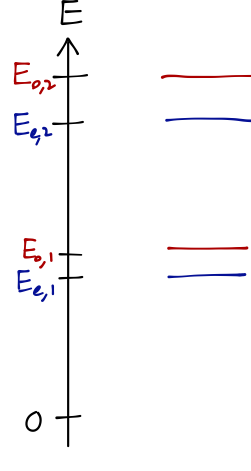
The parity splitting E_{o,1} - E_{e,1} is much smaller than the level splitting E_{e,2} - E_{e,1} (experimentally, by a factor of a thousand or so.) This smallest splitting corresponds exactly to inversion; to see precisely how, we need to go further and look at the time evolution of this system.
You might wonder, what happens to the system when V_0 becomes very small (or equivalently, what do the bound states look like for E \gg V_0?) This limit isn’t relevant for the study of ammonia inversion, but it’s always a good idea to check your limits in any physics calculation.
In the limit that V_0 vanishes we expect to recover results for a single infinite square well of width 2b+a. In fact, as soon as E > V_0 we have to be careful, since the solutions in the barrier region become plane waves, so we have to replace \kappa \rightarrow -ik', where k' = \sqrt{2m(E-V_0)}/\hbar.
With this replacement, and the identities \coth(ix) = -i \cot(x) and \tanh(ix) = i \tan (x), we find the energy conditions become \tan (k_e a) = -\frac{k_e}{k'_e} \cot[-k'_e (b-a/2)] \\ \tan (k_o a) = +\frac{k_o}{k'_o} \tan[-k'_o (b-a/2)]. So what happens when E \gg V_0? Well, first of all we must have k \approx k', which simplifies the equations: \tan (k_e a) = -\cot[-k_e (b-a/2)] \\ \tan (k_o a) = \tan[-k_o (b-a/2)].
Since tangent satisfies the identities \tan(x+\pi/4) = -\cot(x) and \tan(x+\pi/2) = \tan(x), these conditions reduce to k_e a = -k_e (b-a/2) + \pi/4 \\ k_o a = -k_o (b-a/2) + \pi/2 or k_e = \frac{n\pi}{2(a+2b)} \\ k_o = \frac{n\pi}{a+2b}. These lead to exactly the eigenenergies for the infinite square well with width 2b+a, as we expected. The splitting between the even and odd-parity states, which started out very small as we saw for the ground state, becomes larger and larger as n increases (since the energies go as n^2.)
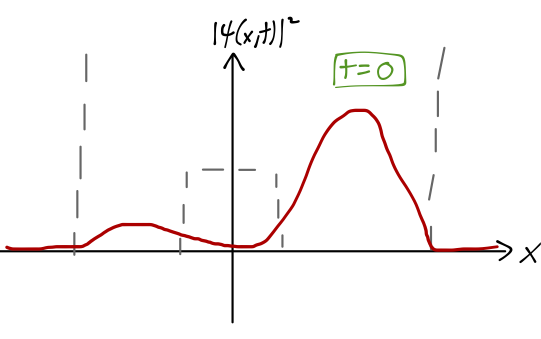
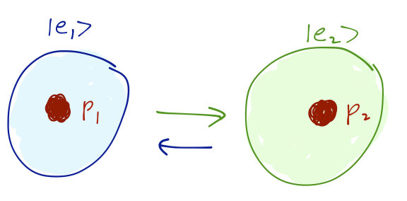
Let’s take our initial state to be localized in the right well: \ket{\psi(t=0)} = \frac{1}{\sqrt{2}} \left[ \ket{\psi_{e,1}} + \ket{\psi_{o,1}} \right] Unlike the infinite-barrier case, the even and odd wavefunctions aren’t equal and opposite in the left well, partly due to the energy difference; so this state is only mostly localized in the right well, as we see from plotting |\psi(x)|^2.
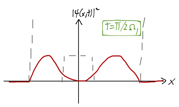
Since we’ve already written our state vector as a sum over energy eigenstates, it’s easy to find the time-evolved state: \ket{\psi(t)} = \frac{1}{\sqrt{2}} \left[ e^{-iE_{e,1} t/\hbar} \ket{\psi_{e,1}} + e^{-iE_{o,1} t/\hbar} \ket{\psi_{o,1}} \right] \\ = \frac{1}{\sqrt{2}} e^{-i(E_{e,1} + E_{o,1})t/(2\hbar)} \left[ e^{i\Omega_1 t/2} \ket{\psi_{e,1}} + e^{-i\Omega_1 t/2} \ket{\psi_{o,1}} \right] where I have defined the quantity \Omega_1 = \frac{E_{o,1} - E_{e,1}}{\hbar}. To find the probability density over time, we take the modulus squared, canceling the overall phase in front and giving us |\psi(x,t)|^2 = |\left\langle x | \psi(t) \right\rangle|^2 = \frac{1}{2} \left( \psi_{e,1}^2 + \psi_{o,1}^2 \right) + \cos (\Omega_1 t) \psi_{e,1}(x) \psi_{o,1}(x). where I’ve simplified knowing that the parity-eigenstate wavefunctions here are real-valued. The effect of the cosine term is that the wavefunction rotates from (\psi_{e,1}(x) + \psi_{o,1}(x)) at t=0, to (\psi_{e,1}(x) - \psi_{o,1}(x)) at t=\pi / \Omega_1 - at which point the wavefunction is localized in the left well.
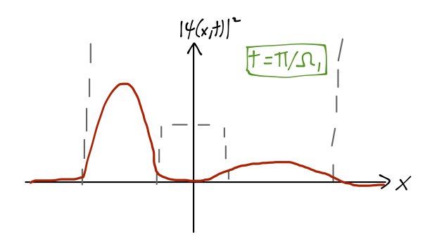
So as the system evolves in time, the position x shifts from localized in the right well, to the left well and back again with frequency f=\Omega_1 / (2\pi). Remembering that x is the distance between the nitrogen atom and the plane of the three hydrogen atoms, and the two potential wells correspond to the two possible orientations of the nitrogen atom, we can see that this motion is exactly the inversion we were looking for. As we’ve observed, the energy difference E_{o,1} - E_{e,1} which determines the inversion frequency is very small, as promised; experimentally, it corresponds to the emission of microwave light.
It’s interesting to think more about the splitting induced by the finite central barrier. Not only did we find separate energies for even and odd parity eigenstates, but the correction to the even-parity state is negative: E_{e,1} < E_1. Thus the ground state of the ammonia molecule is actually more stable than we would have predicted if we were ignoring the possibility of inversion. The stability is associated with the fact that the most stable configuration is not one of the individual minima of the potential, corresponding to the nitrogen being oriented in one direction or another, but rather a quantum superposition of both orientations, symmetrically in this case.
There are plenty of examples of this phenomenon in quantum mechanics; I’ll give you two famous ones. Another interesting molecule is benzene, C_6 H_6. The most stable configuration of this molecule is for the six carbon atoms to form a hexagon; this is confirmed by experiment. Since carbon has four valence electrons, every C should have one bond with a hydrogen atom and three with its carbon neighbors, which means that three of the six sides of the hexagon should be double bonds. It turns out that there are two degenerate configurations with minimum energy:
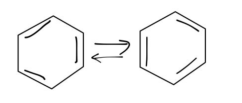
Similar to the inversion of ammonia, it’s possible for benzene to invert between these two configurations. The resulting ground state is more stable than either individual state, and is again a superposition of both possibilities.
Another good example is given by a much simpler molecule, H_2^+; two protons with a single electron orbiting them. Again, if the separation between the protons is very large, we find two configurations of the system with equal energy with the electron localized around one proton or the other, giving a ground-state hydrogen atom. However, as a function of the separation the electron will be able to tunnel from one proton to the other, and the most stable configuration is a superposition. The energy of the combined state is again lower than either individual configuration; this is the source of the molecular bond!
(I’ve given my attempt at describing this phenomenon, but I can’t possibly beat Richard Feynman, so if you’d like to read more I recommend reading the explanation in his words.)
9.3 The two-state description
We can learn more about the inversion of ammonia by isolating the two energy eigenstates E_{e,1} and E_{o,1} and treating them as a two-state system, ignoring all of the other states. Let’s take as a basis the two states \ket{\psi_L^1} and \ket{\psi_R^1} which correspond to a localized particle in the left or right well, respectively. Since we’re only considering two states, the entire Hilbert space is spanned by these two kets.
(For the more mathematically inclined, I’ll warn you that what we’re about to do is phenomenology; we will use what we learned in our wave mechanics example to describe the two-state system of the lowest inversion states. The rigorous justification for doing this will have to wait until we study perturbation theory, but for now you’ll just have to accept that we can ignore the other eigenstates because they’re relatively well-separated in energy.)
Let’s being by looking back at what we did with an infinite potential barrier. In this case, we found the two basis states (the ground states in each well) are orthogonal and have the same energy E_1. The Hamiltonian matrix is therefore just \hat{H}_0 = \left(\begin{array}{cc} E_1 & 0 \\ 0 & E_1 \end{array} \right). When the barrier was lowered to V_0, we noted that the states \ket{\psi_L^1} and \ket{\psi_R^1} were no longer orthogonal to each other; a particle localized in one well has a finite probability of being transmitted through the barrier to the other well. This means that in the presence of a finite barrier, our two-state Hamiltonian in this basis can’t be diagonal. So we must now have \hat{H} = \left( \begin{array}{cc} E_1 & -A \\ -A & E_1 \end{array} \right) with A>0. The fact that the off-diagonal entry A is real is guaranteed by parity (this is a simple exercise using the definition of parity and the Hermiticity of \hat{H}.) As for the sign of A, the difference is phenomenological: the sign dictates whether the even-parity or odd-parity states are lighter. There is no right answer in general, but we know for this problem that the even-parity states are lighter, giving the structure here.
We’ve already solved the most general two-state Hamiltonian, so I’ll just invoke the solution here. Given a Hamiltonian \hat{H} = \left( \begin{array}{cc} \epsilon_1 & \delta \\ \delta^\star & \epsilon_2 \end{array} \right) the energy eigenvalues are E_{\pm} = \frac{\epsilon_1 + \epsilon_2}{2} \pm \sqrt{\left(\frac{\epsilon_1 - \epsilon_2}{2} \right)^2 + |\delta|^2} and the eigenkets are determined by the mixing matrix \left( \begin{array}{cc} \cos \theta & \sin \theta (\delta^\star/|\delta|) \\ -\sin \theta (\delta/|\delta|) & \cos \theta \end{array} \right) acting on the initial basis. Finally, the mixing angle is given by \tan 2\theta = \frac{2|\delta|}{\epsilon_1 - \epsilon_2}. We see that having \epsilon_1 = \epsilon_2 and \delta real makes things particularly simple: since \tan 2\theta is infinite, we have \theta = \pi/4, giving the maximally-mixed eigenstates \ket{+} = \frac{1}{\sqrt{2}} (\ket{\psi_L^1} - \ket{\psi_R^1}) = \ket{\psi_o^1} \\ \ket{-} = \frac{1}{\sqrt{2}} (\ket{\psi_L^1} + \ket{\psi_R^1}) = \ket{\psi_e^1}, and the energy eigenvalues are E_{\pm} = E_1 \pm A. (Don’t forget the minus sign in the mixing matrix! Even though \delta = -A is real, we still have \delta^\star / |\delta| = -A/A = -1.)
This reproduces exactly the results we found with our more detailed analysis; namely, that lowering the central potential barrier causes the degeneracy between the energies to be split, and the new energy eigenstates are symmetric and antisymmetric combinations of the single-well states, with the symmetric state having lower energy.
We also find the same time evolution: if we start in the same initial state \ket{\psi(t=0)} = \ket{\psi_R^1} = \frac{1}{\sqrt{2}} [\ket{\psi_e^1} + \ket{\psi_o^1}] then the time-evolved state is \ket{\psi(t)} = \frac{1}{\sqrt{2}} e^{-iE_1 t/\hbar} [e^{iAt/\hbar} \ket{\psi_e^1} + e^{-iAt/\hbar} \ket{\psi_o^1} \\ = e^{-iE_1t/\hbar} \left[ \cos \left( \frac{At}{\hbar} \right) \ket{\psi_R^1} + i \sin \left( \frac{At}{\hbar} \right) \ket{\psi_L^1} \right]. So we see inversion between the two local states once again, and can identify the inversion angular frequency \Omega_1 = 2A/\hbar.
9.4 Ammonia in an electric field
Now that we have a simplified two-state model, we can make things a little more interesting by adding an external electric field \mathcal{E} to our two-state system. When the nitrogen atom is localized on one side or another of the hydrogens, it gives the molecule a net electric dipole moment, which can be expressed as an operator, \hat{D} = \left( \begin{array}{cc} -\mu & 0 \\ 0 & \mu \end{array} \right). I’ll remind you that the classical electric dipole moment (EDM) is just the average of the charge density times the displacement, e.g. for point charges \vec{D} = \sum_i q_i \vec{x}_i. Clearly for ammonia this tells us that the EDM should be equal and opposite in the two inverted configurations, hence the form of the operator above.
The interaction of the ammonia electric dipole with an applied electric field has the Hamiltonian \hat{H}_{ED} = \mathcal{E} \hat{D}. (For simplicity I’m assuming the electric field is aligned with the axis of the molecule.) Thus, the total Hamiltonian of the system is now \hat{H} = \left( \begin{array}{cc} E_1 - \mu \mathcal{E} & -A \\ -A & E_1 + \mu \mathcal{E} \end{array} \right), giving the energy eigenvalues E_\pm = E_1 \pm \sqrt{A^2 + \mu^2 \mathcal{E}^2} and the mixing angle is now \tan 2\theta = A / (\mu \mathcal{E}). When \mathcal{E} \gg A, the energy varies linearly with \mathcal{E}, and the eigenstates become localized to \ket{\psi_L^1} or \ket{\psi_R^1}; the applied external field pulls the nitrogen to one side or the other. If we plot the energies versus the applied field, we see the expected avoided level crossing; the finite barrier for the two localized states to tunnel into one another, represented by interaction A, breaks the would-be degeneracy at \mathcal{E} = 0.
It’s interesting to calculate the expectation values of the electric dipole moment itself in the two energy eigenstates. It’s straightforward to show that \bra{\psi_e^1} \hat{D} \ket{\psi_e^1} = - \bra{\psi_o^1} \hat{D} \ket{\psi_o^1} = \mu \cos (2\theta) = -\frac{\mu^2 \mathcal{E}}{\sqrt{A^2 + \mu^2 \mathcal{E}^2}}. The ammonia molecule thus has only an induced electric dipole moment; if the external field vanishes, then so does \left\langle D \right\rangle. This is because the energy eigenstates correspond to (anti-)symmetric combinations of the single-well wavefunctions, so that the nitrogen atom has an equal probability of being on either side of the hydrogens, giving zero net dipole moment.
The vanishing of the permanent EDM of the parity eigenstates is actually an example of a very general statement based on parity. Let’s step back from our example for a moment and suppose that we have any two parity eigenstates, \ket{\alpha} and \ket{\beta}: \hat{P} \ket{\alpha} = \epsilon_\alpha \ket{\alpha} \\ \hat{P} \ket{\beta} = \epsilon_\beta \ket{\beta} where as we know the eigenvalues are \epsilon_\alpha, \epsilon_\beta = \pm 1. We saw that certain operators have definite properties under parity transformation, in particular the position operator is odd, \hat{P} \hat{x} \hat{P}{}^{-1} = -\hat{x}. The matrix element of \hat{x} with respect to the two parity eigenstates is thus \bra{\beta} \hat{x} \ket{\alpha} = \bra{\beta} (\hat{P}^{-1} \hat{P}) \hat{x} (\hat{P}^{-1} \hat{P}) \ket{\alpha} \\ = \epsilon_\alpha \epsilon_\beta (-\bra{\beta} \hat{x} \ket{\alpha}). Therefore, if the two states have the same parity \epsilon_\alpha = \epsilon_\beta, then we find \bra{\beta} \hat{x} \ket{\alpha} = 0. This is a specific example of a selection rule. The name comes from application to systems such as transitions between atomic levels, where the atom will “select” only certain possible transition outcomes. In general, a selection rule is a statement that certain matrix elements must vanish based on symmetry considerations.
To tie back to our discussion, as we noted the dipole moment of a charge distribution is linearly propotional to \hat{\vec{x}}, which means that it is also odd under parity. Since many atomic transitions involve electric dipole moments (as we will see later on), this statement for \hat{\vec{x}} is a direct constraint on radiative transitions in atoms. We can also observe that for any parity eigenstate, we always have \bra{\alpha} \hat{x} \ket{\alpha} = 0. Thus for any system in which the Hamiltonian is parity invariant, all of the non-degenerate energy eigenstates satisfy this equation, and so they cannot possess any permanent EDM (as is the case for our two-state ammonia example.)
In practice, the electric field \mathcal{E} will be fairly weak, such that \mu \mathcal{E} \ll A, which means that we can expand to find E_+ = E_{o,1} \approx E_1 + A + \frac{\mu^2 \mathcal{E}^2}{2A}, \\ E_- = E_{e,1} \approx E_1 - A - \frac{\mu^2 \mathcal{E}^2}{2A}. Once again, we see that where a particle with a static dipole moment would have energy proportional to \mathcal{E}, the ammonia molecule has energy proportional to \mathcal{E}^2. The coefficient \mu^2 / 2A is known as the polarizability of our molecule, and it determines how strongly it responds to application of an external electric field. The physical picture you should have here is that while an ordinary dipole moment corresponds to a distribution of charge which is asymmetric in some way, polarizability only requires some sort of free charge distribution to be present; these charges are “pulled apart” by the external field when it is applied.
The force felt by the ammonia molecule in the presence of a field with a spatial gradient is proportional to the gradient of the polarizability, \vec{F} = \frac{\mu^2}{2A} \nabla (\mathcal{E}^2). It so happens that A is relatively small for ammonia, which means that (compared to many other molecules) ammonia is quite sensitive to applied electric fields.
We can make use of this interaction to build a Stern-Gerlach-like beam splitter, which will separate the \ket{\psi_e^1} and \ket{\psi_o^1} states spatially. This is the first step in constructing an ammonia maser. If we can isolate a beam of molecules in the higher-energy \ket{\psi_o^1} state, then we pass the beam through a cavity which has an electromagnetic field oscillating at exactly the right frequency in time, all of the excited-state ammonia molecules can be induced to transition back to the lower state with probability 1 in the time it takes to traverse the cavity. As a result, the excess (microwave-frequency) energy is emitted into the cavity, converting molecular energy into the energy of an external electromagnetic field, and thus microwave light.
(Practically, the efficiency will be much lower than 100%; even if we prepare a pure initial state, the molecules will have a distribution of velocities, and so we won’t be able to reliably induce the transition inside the cavity. There are much more practical ways of making lasers, but we’ll come back to those when we study time-dependent electromagnetic interactions later.)