Appendix D — Berry phase
The fact that energy eigenstates don’t mix together under adiabatic evolution is not that surprising. The larger surprise from the derivation above is the existence of the geometric phase, also known as Berry’s phase or simply a Berry phase. It depends on time only implicitly, in terms of the path taken through parameter space defined by \theta^i(t) (so the “geometry” on which it depends is the geometry of our fictitious parameter space, not the real geometry of space and time.) In some references, “Berry phase” will refer specifically to the case in which we follow a closed loop in parameter space where we return the system to where we started, so \theta(t) = \theta(0): \gamma_n = \oint_{\mathcal{C}} d\vec{\theta} \cdot \vec{\mathcal{A}}^n(\theta). where \mathcal{C} is a closed-loop path through parameter space. In this case the instantaneous energy eigenstates are the same before and after the evolution, \ket{E_n(t)} = \ket{E_n(0)}. But there is still a change to the quantum state, on top of the expected dynamical phase e^{-iE_n t/\hbar}; the system has some additional “memory” of how the parameters were changed, encoded in the Berry phase.
For the rest of this subsection, we’ll drop the index n and just focus on a single energy eigenstate, \ket{E_n(t)}. Restoring the parameter-space index, the Berry phase associated with evolution of this state is then \gamma = \oint_{\mathcal{C}} d\theta^i \mathcal{A}_i. This is, as we have already observed, completely independent of the specific parametrization \theta(t), only depending on the path through parameter space. But it is also invariant under certain other changes we can make. In particular, consider a modification of the Berry connection of the form \mathcal{A}_i' = \mathcal{A}_i + \frac{\partial \omega}{\partial \theta^i} for some function \omega(\theta). If we plug this back in to the formula for the Berry phase, \gamma' = \oint_{\mathcal{C}} d\theta^i \mathcal{A}_i' = \oint_{\mathcal{C}} d\theta^i \mathcal{A}_i + \oint_{\mathcal{C}} d\theta^i \frac{\partial \omega}{\partial \theta^i} \\ = \gamma + \oint_{\mathcal{C}} d\omega = \gamma with the d\omega integral vanishing since we come back to the same point, so the result is \omega(\theta) - \omega(\theta) = 0. So the Berry phase is invariant under such a change to the connection. This is good news, since a change of this form arises from a remaining ambiguity that we haven’t dealt with. Specifying the parameterization \theta(t) fixes the problem we raised above with the instantaneous energy eigenstates \ket{E_n(t)} picking up an arbitrary time-dependent phase e^{i\phi(t)}. But after the parameterization, we can still add an arbitrary phase to the eigenstates as long as it depends on \theta and not t directly: \ket{E_n(\theta)} \rightarrow e^{i\omega(\theta)} \ket{E_n(\theta)} gives an equivalent description of the physics. This rephasing causes a change to the Berry connection precisely as we wrote above, but doesn’t change the Berry phase. As we saw with gauge symmetry, this is an unphysical redundancy of our description, and so there cannot be physical consequences to the arbitrary changes given by \omega(\theta).
All of this should strongly remind you of our discussions of gauge symmetries; the Berry phase itself is very similar to the phase that appears in the Aharonov-Bohm effect. The key difference is that gauge symmetry is a symmetry involving paths through real space, while the Berry phase comes from paths through some parameter space. The mathematics used to describe these two different phenomena is very similar.
D.0.1 Example: neutron in a magnetic field
Let’s work through a simple example, looking at a single neutron in an external magnetic field, treating it as a two-state system. (Neutrons are spin-1/2 like electrons, but also electrically neutral, so we don’t have to worry about other ways they interact with the magnetic field in an experiment; for the purposes of the calculation we’re going to do here, they are treated the same.) We have already exhaustively looked at the time dependence of this system for various types of applied magnetic field, even certain time-dependent ones. But now, we’ll study what happens if the direction of the applied magnetic field is slowly rotated.
The Hamiltonian for this system takes the form \hat{H} = \frac{\hbar \omega}{2} \hat{\vec{\sigma}} \cdot \frac{\vec{B}}{|\vec{B}|} with \omega \equiv eg_n|\vec{B}|/(2m_nc). As we have already found (see Section 4.1.2), if we take the magnetic field direction described by \vec{B}/|\vec{B}| to be given by the spherical angles \theta and \phi, then the energy eigenstates are \ket{+} = \left( \begin{array}{c} \cos (\theta/2) \\ \sin (\theta/2) e^{i \phi} \end{array} \right), \\ \ket{-} = \left( \begin{array}{c} -\sin (\theta/2) \\ \cos (\theta/2) e^{i \phi} \end{array} \right), with corresponding energy eigenvalues E_\pm = \pm \hbar \omega/2.
So far this is all for a fixed magnetic field vector \vec{B}, but now we can take the magnetic field components (B_x, B_y, B_z) to be our parameter vector \theta^i. Allowing some slow time variation \vec{B}(t) then gives us the time-dependent Hamiltonian \hat{H}(t) we want, with the parameterization already built in. For this calculation, we’ll switch to spherical coordinates (|B|, \theta_B, \phi_B) in our parameter space as well. (It so happens that the way we have set things up, \theta_B and \phi_B are exactly the spherical angles describing the direction that the \vec{B}-field is pointing in real space as well, but don’t get confused; in general the parameter space is entirely separate!)
First of all, by the adiabatic theorem we’re guaranteed that if we begin in one of the energy eigenstates, we will stay in that state for all time. Let’s take the state \ket{+} to be our initial state; the results will of course be basically the same if we use \ket{-} instead.
One of the features we discussed previously regarding the two-state system solutions is that the energy eigenstates can “switch places” depending on exactly what the Hamiltonian looks like - in the solution of Section 4.3, this happens depending on the phase of the off-diagonal element \delta. Indeed, we can just plug in some specific choices of spherical angles above to see this effect: if we take \theta = \pi/2 and \phi = 0, then \ket{+} \rightarrow \frac{1}{\sqrt{2}} \left( \begin{array}{c} 1 \\ 1 \end{array} \right) \\ \ket{-} \rightarrow \frac{1}{\sqrt{2}} \left( \begin{array}{c} -1 \\ 1 \end{array} \right) \\ but if we change the phase to \phi = \pi, then \ket{+} \rightarrow \frac{1}{\sqrt{2}} \left( \begin{array}{c} 1 \\ -1 \end{array} \right) \\ \ket{-} \rightarrow \frac{1}{\sqrt{2}} \left( \begin{array}{c} 1 \\ 1 \end{array} \right) \\ So changing the phase causes our two eigenstates to switch places: \ket{S_{x,+}} is the negative energy state \ket{+} at \theta = \pi/2, but it’s the positive energy state \ket{-} if \theta = 0.
The key point to realize here is that although the two energy eigenstates “switch places” in terms of the \hat{S}_z basis (or any other basis) as we vary the angle, what the adiabatic theorem guarantees is that they vary smoothly as they swap. In other words, if we start in \ket{+} = \ket{S_{x,-}} at \theta = 0 and then slowly change the Hamiltonian until \theta = \pi/2, we will stay in \ket{+} - the energy won’t change - but the state vector will switch to \ket{S_{x,+}}.
Given a path \mathcal{C} through parameter space, then, the resulting Berry phase will be \gamma = \oint_{\mathcal{C}} d\theta^i \mathcal{A}_i = \oint_{\mathcal{C}} (|B| d\theta_B \mathcal{A}_\theta + |B| \sin \theta_B d\phi_B \mathcal{A}_\phi), substituting in the spherical line element in parameter space - it may be a fictitious space, but we still have to keep track of geometric factors when we change coordinates!
Now we need the value of the Berry connection, which is easily computed since we have the instantaneous eigenstates. However, we do have to be careful about geometric factors again: the general definition of the Berry connection is \vec{\mathcal{A}}^n = i \bra{n(\theta)} \vec{\nabla}_\theta \ket{n(\theta)} which means that in our spherical coordinates, \mathcal{A}_\theta^+ = \frac{i}{|B|} \bra{+} \frac{\partial}{\partial \theta_B} \ket{+} = 0, \\ \mathcal{A}_\phi^+ = \frac{i}{|B| \sin \theta_B} \bra{+} \frac{\partial}{\partial \phi_B} \ket{+} = -\frac{\sin^2 (\tfrac{\theta_B}{2})}{|B| \sin \theta_B}. \\ This is everything we need to calculate the Berry phase for a given curve \mathcal{C}. A simple and interesting class of curves \mathcal{C}_\theta are defined by holding \theta_B fixed at some angle, and then varying \phi in a complete circle from 0 to 2\pi. The resulting Berry phase is \gamma_\theta^+ = |B| \int_0^{2\pi} d\phi_B \sin(\theta_B) \left(-\frac{\sin^2 (\tfrac{\theta_B}{2} )}{|B| \sin (\theta_B)}\right) \\ = -2\pi \sin^2(\theta_B/2) = -\frac{\Omega_B}{2}, where \Omega_B is precisely the solid angle subtended by the part of the sphere within the curve \mathcal{C}_\theta. (For example, if we take an equatorial path \theta_B = \pi/2, the solid angle subtended is 2\pi - half of the entire sphere - and the resulting Berry phase is -\pi.) If we repeat the calculation for the other energy eigenstate, we find the result \gamma_\theta^- = -2\pi \cos^2(\theta_B/2) = -2\pi (1 - \sin^2(\theta_B/2)) = - \frac{(4\pi - \Omega_B)}{2}.
What is the physical consequence of this phase? If we just have a single initial state \ket{\psi} and track its evolution, the Berry phase is unobservable since it amounts to an overall global phase. To observe its presence, we need to compare to a second state that doesn’t have the phase. Let’s consider a Mach-Zehnder interferometer as the setup:
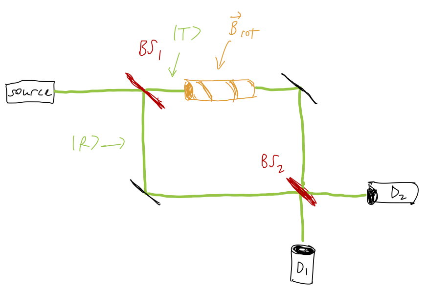
Our input beam encounters a beam splitter, which has the effect of splitting it into two beams, reflected R and transmitted T. Since there are two paths along which our particles can propagate from input to output, we can effectively describe this experiment in terms of a two-state Hilbert space consisting of \ket{R} and \ket{T}. The beam splitter itself can be described as a unitary operation that maps the two input states \ket{I_1}, \ket{I_2} to the output states \ket{O_1}, \ket{O_2} as \hat{U}_{BS} = \frac{1}{\sqrt{2}} \left( \begin{array}{cc} 1 & i \\ i & 1 \end{array} \right). Now, suppose we have an input beam of neutrons prepared in the state \ket{-}. After the first beam splitter, the state of the system becomes \ket{\psi_{MZ,{\rm in}}} = \frac{1}{\sqrt{2}} (\ket{R} + i\ket{T}) \otimes \ket{-} where we have a direct-product state encoding the spatial state times the spin state. Next, as pictured, we subject the transmitted arm of the interferometer to a time-varying rotating magnetic field of magnitude |B_{\rm rot}| in the xy plane, while the other arm remains in a constant magnetic field; we set things up in such a way that |\vec{B}| is held fixed everywhere. In propagating from the first to second beam splitter, then, each arm will pick up a dynamical phase, \xi_R(t) = \frac{1}{\hbar} \int_0^L dt' E_n(t') = -\frac{\omega t}{2} where L is the length of the path of travel and \xi_T = \xi_R since the magnetic field strength is fixed. The transmitted state only will pick up a geometric phase as well, according to the solid angle subtended by the magnetic field rotation. Thus, at the input to the second beam splitter, we have \ket{\psi_{MZ,{\rm out}}} = \frac{1}{\sqrt{2}} \left( e^{-i\omega t/2} \ket{R} \otimes \ket{-} + ie^{-i\omega t/2} e^{-i\Omega_B/2} \ket{T} \otimes \ket{-} \right) Applying the second beam splitter as another unitary operator (on the spatial components) relates this state to the output states at detector 1 or detector 2, \ket{\psi_f} = \frac{1}{2} e^{-i\omega t/2} \left[ (1-e^{-i\Omega_B/2}) \ket{D_1} + i(1+e^{-i\Omega_B/2}) \ket{D_2} \right]. Now if we read out, say, detector 1, we find the neutron with probability p(D_1) = |\left\langle D_1 | \psi_f \right\rangle|^2 = \frac{1}{4} |1-e^{-i\Omega_B t/2}|^2 = \frac{1}{2} - \frac{1}{2} \cos \left( \frac{\Omega_B}{2} \right).
Although the setup that I’ve given here is plausible, realistic experimental measurements of the Berry phase using neutrons (see e.g. this paper by Bitter and Dubbers) use different setups that are a bit more complicated to describe. There have also been Berry phase measurements done using an interferometer setup like this, but generally using photons and not neutrons.
In the limit that we take the solid angle to be the entire sphere, \Omega_B \rightarrow 4\pi, we find that the Berry phase is -2\pi. This might not seem remarkable, but it is a manifestation of a powerful and general result, which is that if we integrate over any curve that defines a closed surface (in this example, the entire sphere), the resulting Berry phase is always an integer multiple of 2\pi, \gamma_{\rm closed} = 2\pi C, where the integer C is known as the Chern number. There are deep connections to the mathematics of electromagnetism and gauge theory here, and this result can be understood and proved in terms of fictitious ``monopole charges’’ and Gauss’s law, but in the parameter space and not in real space! If you’d like to read more about this I recommend (as I often do here) the discussion in David Tong’s advanced quantum lecture notes.