17 Aspects of time evolution and density matrices
Now that we know the basics of how to work with density matrices, we’ll explore some interesting phenomena that occur once we study how they evolve in time. In particular, considering how measurement interacts with time evolution will lead us to the quantum Zeno effect, while a brief detour into open quantum systems will let us briefly consider the phenomenon of decoherence.
Before we see these more interesting topics, we first need to understand how time evolution acts on density matrices without any of these complications. If we think about the time evolution of our state vectors, then the density matrix will inherit time dependence as well. Working in the Schrödinger picture, the time-dependent density matrix will be \hat{\rho}(t) = \sum_i p_i \ket{\psi_i(t)} \bra{\psi_i(t)} \\ = \sum_i p_i \hat{U}(t) \ket{\psi_i(0)} \bra{\psi_i(0)} \hat{U}^\dagger(t) \\ = \hat{U}(t) \hat{\rho}(0) \hat{U}^\dagger(t). Taking a time derivative gives us the equation of motion \frac{\partial \hat{\rho}}{\partial t} = \frac{1}{i\hbar} [\hat{H}, \hat{\rho}]. This equation is known as the quantum Liouville-von Neumann equation. Note that this is almost the Heisenberg equation for the density matrix, except that it has the wrong sign (in the Heisenberg equation for \hat{O}, the commutator on the right is [\hat{O}, \hat{H}].) This is because we’re working in Schrödinger picture, and \hat{\rho}(t) is defined directly from our state vectors \ket{\psi(t)}.
17.1 Measurement, revisited
Let’s return one more time to our discussion of measurements to add a couple of more observations. When we’re dealing with mixed states, we have two sources of uncertainty: classical uncertainty in the state, and then the usual quantum uncertainty in the outcome of a given measurement. For the latter, we know that measuring eigenvalue a of observable \hat{A} causes the state to collapse via the corresponding projection operator \hat{P}_a. In fact, this is relying on the fact that we can write the operator \hat{A} itself in terms of its own eigenvalues and projectors as \hat{A} = \sum_a a \hat{P}_a. This is known as the spectral decomposition of \hat{A}.
It turns out that we can use the same projection operator to conveniently handle both sources of uncertainty at once. This isn’t really an update of the measurement postulate, it just follows from what we’ve defined so far:
Given an observable \hat{A}, the probability of measuring outcome a in a system described by density matrix \hat{\rho} is p(a) = {\rm Tr} (\hat{\rho} \hat{P}_a), where \hat{P}_a is the projection operator corresponding to outcome a. After measurement, the system collapses to \hat{\rho} \rightarrow \frac{1}{p(a)} \hat{P}_a \hat{\rho} \hat{P}_a.
As with wavefunctions, the collapse of our density matrix through projection is a violent and non-unitary way for our system to evolve in response to measurements. However, this actually opens up some interesting physical effects for us to look at. For one thing, since most measurements have multiple outcomes, saying what happens to our system after a measurement is complicated by keeping track of the multiple possible states after collapse. But with density matrices, we can deal with the situation where we measure \hat{A} but keep all of the outcomes together in our system; the result is the mixed state
\hat{\rho} \rightarrow \sum_a p(a) \left( \frac{\hat{P}_a \hat{\rho} \hat{P}_a}{p(a)} \right) = \sum_a \hat{P}_a \hat{\rho} \hat{P}_a.
17.2 The Quantum Zeno effect
This brings us to the idea of considering the impacts of measurement itself on our system, not just thinking about the outcomes. If we consider a system with both unitary time evolution and applied measurements, the full time evolution of the system will be a result of both effects.
Suppose that we consider a specific measurement \hat{B} that collapses to an non-degenerate eigenstate \ket{b}, which is not an eigenstate of the Hamiltonian. If we measure once and find \ket{b}, and then let the system evolve in time, it will evolve in some unitary way away from \ket{b} according to its energy-eigenstate decomposition. But now suppose we measure repeatedly and find the result b over and over. After every measurement, the state collapses back to \ket{b} and the time evolution has to start over.
The basic idea of slowing down the time evolution using measurements to “reset” the state is known as the quantum Zeno effect, after Zeno’s paradox (in which a turtle takes successively smaller and smaller steps and is thus never able to reach its destination.) However, realization of the Zeno effect requires the measurement outcome to stay the same every time we measure, so we return to the same \ket{b}. But due to the unitary time evolution not preserving this state, there will be a non-zero chance that the system just jumps to another eigenstate when we measure - not a desirable effect if we’re looking to use the Zeno effect to keep the system in a certain state.
We can get a better understanding of the quantum Zeno effect, one which is closer to how it is actually realized in experiment, by using density matrices instead. Density matrices allow us to work with the system as a whole, no matter the measurement outcomes. We’ll do a simple two-state system example to illustrate what happens. Suppose our two-state system has Hamiltonian \hat{H} = \frac{\hbar \omega}{2} \left( \begin{array}{cc} 1 & 0 \\ 0 & -1 \end{array} \right), and we take the initial state to be spin-up in the x direction, \ket{\psi(0)} = \ket{\rightarrow} = \frac{1}{\sqrt{2}} (\ket{\uparrow} + \ket{\downarrow}). If we let this state evolve in time, we know the answer is \ket{\psi(t)} = \frac{1}{\sqrt{2}} (e^{-i\omega t/2} \ket{\uparrow} + e^{+i\omega t/2} \ket{\downarrow}), so that \left\langle \psi(0) | \psi(t) \right\rangle = \cos \frac{\omega t}{2}. We see that as the system evolves in time, the overlap of \ket{\psi(t)} with the \ket{\rightarrow} state decreases (until things turn around and return to the original state for t > \pi/\omega, at least in an ideal situation.) Can we slow this down with the quantum Zeno effect by making some measurements?
This question will be much easier to answer using density matrices, so let’s switch over to that. The original density matrix is \hat{\rho}(0) = \ket{\psi(0)} \bra{\psi(0)} = \frac{1}{2} \left( \begin{array}{cc} 1 & 1 \\ 1 & 1 \end{array} \right) \\ = \frac{1}{2} \hat{1} + \frac{1}{2} \hat{\sigma}_x, writing a decomposition in terms of Pauli matrices which will be useful to work with: in general, we can write \hat{\rho} = \rho_1 \hat{1} + \rho_x \hat{\sigma}_x + \rho_y \hat{\sigma}_y + \rho_z \hat{\sigma}_z and then \rho_1(0) = \rho_x(0) = 1/2. For the time evolution, we have the Liouville equation \frac{d\hat{\rho}}{dt} = \frac{1}{i\hbar} [\hat{H}, \hat{\rho}] \\ = -\frac{i\omega}{4} [\hat{\sigma}_z, \hat{\rho}] \\ = \frac{\omega}{2} (\rho_x \hat{\sigma}_y - \rho_y \hat{\sigma}_x), from which we read off that \dot{\rho}_1 = \dot{\rho}_z = 0, and the coupled system \dot{\rho}_x = -\tfrac{\omega}{2} \rho_y, \\ \dot{\rho}_y = +\tfrac{\omega}{2} \rho_x. Assuming only unitary evolution and no measurement yet, this gives us a time-dependent density matrix of the form \hat{\rho}_U(t) = \frac{1}{2}\left( \begin{array}{cc} 1 & e^{-i\omega t/2} \\ e^{+i\omega t/2} & 1 \end{array}\right). Instead of looking at the overlap with the initial state, let’s just consider the expectation value of x-direction spin, \left\langle \hat{\sigma}_x \right\rangle. This contains the same information since it is equal to +1 in the initial state and decreases as the system evolves in time. As a check on our density matrix, we have \left\langle \hat{\sigma}_x \right\rangle = {\rm Tr} (\hat{\sigma}_x \hat{\rho}(t)) \\ = {\rm Tr} \left( \begin{array}{cc} 1/2 e^{-i\omega t/2} & 1/2 \\ 1/2 & 1/2 e^{+i\omega t/2} \end{array} \right) = \cos \frac{\omega t}{2}.
Now we add in our measurement. Suppose that we measure \hat{\sigma}_x, but don’t separate things out based on the outcome, keeping our system unchanged. Then from above, the effect of projection will be \hat{\rho} \rightarrow \hat{P}_{\rightarrow} \hat{\rho} \hat{P}_{\rightarrow} + \hat{P}_{\leftarrow} \hat{\rho} \hat{P}_{\leftarrow}, where the projection matrices are \hat{P}_\rightarrow = \ket{\rightarrow} \bra{\rightarrow} = \frac{1}{2} \left(\begin{array}{cc} 1 & 1 \\ 1 & 1 \end{array} \right) \\ = \frac{1}{2} (\hat{1} + \hat{\sigma}_x), \\ \hat{P}_\leftarrow = \ket{\leftarrow} \bra{\leftarrow} = \frac{1}{2} \left(\begin{array}{cc} 1 & -1 \\ -1 & 1 \end{array} \right) \\ = \frac{1}{2} (\hat{1} - \hat{\sigma}_x). If you work this out using some Pauli matrix algebra, you will find that in the parameterization given above, the effect of this projection is to set \rho_y, \rho_z = 0 while leaving the other two components of the density matrix untouched.
Do the algebra and demonstrate that projection due to the unfiltered \hat{\sigma}_x measurement does as described above.
Answer:
In terms of Pauli matrices, we have \hat{\rho} \rightarrow \frac{1}{4} (\hat{1} + \hat{\sigma}_x) \hat{\rho} (\hat{1} + \hat{\sigma}_x) + \frac{1}{4} (\hat{1} - \hat{\sigma}_x) \hat{\rho} (\hat{1} -\hat{\sigma}_x) \\ = \frac{1}{2} \hat{\rho} + \frac{1}{2} \hat{\sigma}_x \hat{\rho} \hat{\sigma}_x, cancelling off the terms with one \hat{\sigma}_x. We can rewrite this further using a commutator as \hat{\rho} \rightarrow \hat{\rho} + \frac{1}{2} \hat{\sigma}_x [\hat{\rho}, \hat{\sigma}_x]. Now we need to find that commutator. Let’s expand out \hat{\rho} in terms of our matrix basis, and just keep the non-vanishing commutators: [\hat{\rho}, \hat{\sigma}_x] = [\rho_y \hat{\sigma}_y + \rho_z \hat{\sigma}_z, \hat{\sigma}_x] \\ = 2i\rho_y \epsilon_{yxz} \hat{\sigma}_z + 2i \rho_z \epsilon_{zxy} \hat{\sigma}_y \\ = 2i (\rho_z \hat{\sigma}_y - \rho_y \hat{\sigma}_z). Finally, we multiply by \hat{\sigma}_x on the left, \hat{\sigma}_x [\hat{\rho}, \hat{\sigma}_x] = 2i (\rho_z \hat{\sigma}_x \hat{\sigma}_y - \rho_y \hat{\sigma}_x \hat{\sigma}_z) \\ = 2i (\rho_z i\epsilon_{xyz} \hat{\sigma}_z - \rho_y i \epsilon_{xzy} \hat{\sigma}_y) \\ = -2 \rho_y \hat{\sigma}_y - 2\rho_z \hat{\sigma}_z. Plugging back in above, this cancels the y and z components off exactly, so we have simply \hat{\rho} \rightarrow \rho_1 \hat{1} + \rho_x \hat{\sigma}_x.
Note that this doesn’t change the expectation value \left\langle \hat{\sigma}_x \right\rangle at all - as we should expect, since without any time evolution repeated measurement of this operator should always give the same result. But with unitary time evolution added, if we track \left\langle \hat{\sigma}_x(t) \right\rangle, measurement won’t cause any sudden jumps, but it will alter the time evolution by zeroing out the \rho_y component.
At this point we need to resort to numerical solution, since the measurements aren’t described by a nice analytic function, they are impulses applied at specific times. But we have all the analytic pieces above needed to implement a numerical solution in Mathematica. Here is the result:
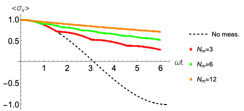
We can clearly see the Zeno effect; as we apply 3, 6, and 12 measurements within the timespan of a single half-period t = \pi / (\omega/2), the evolution becomes slower and slower, so that the system remains closer to the initial state \ket{\rightarrow}.
17.3 Open quantum systems
We have seen a fair bit of formalism for how density matrices can be used to describe bipartite quantum systems \mathcal{H} = \mathcal{H}_A \otimes \mathcal{H}_B, testing for entanglement and so on. Now I’d like to consider a specific bipartite system, which is an open quantum system, \mathcal{H} = \mathcal{H}_S \otimes \mathcal{H}_E. Here \mathcal{H}_S is a quantum system that we’re interested in, and \mathcal{H}_E represents the environment. Any realistic quantum experiment that we want to do always exists in the presence of an environment, so this is a useful setup for thinking about it. Typically we would have d(\mathcal{H}_E) \gg d(\mathcal{H}_S), that is, the environment is an enormous Hilbert space, like a thermal reservoir if we were doing statistical mechanics.
Suppose that we initialize our system \mathcal{H}_S into a pure state \ket{\psi}. If we only had the system itself (i.e. if there was no contact with the environment), then it would evolve ideally according to the Schrödinger equation. However, now we immerse the system in an environment, which means that the initial state is larger, \ket{\Psi(0)} = \ket{\psi}_S \otimes \ket{\phi}_E (we’ll assume that the whole system begins in a pure state, to begin with, and with no entanglement between the system and the environment.) Again, if the Hamiltonian itself is purely bipartite, \hat{H} = \hat{H}_S \otimes \hat{H}_E, then the time evolution of \ket{\psi}_S just follows the Schrödinger equation according to the system Hamiltonian. But this is only true if the environment is perfectly shielded; in general, there will be some off-diagonal parts of the Hamiltonian connecting \mathcal{H}_S and \mathcal{H}_E, which will complicate the time evolution.
Since we are just interested in what happens to the system and want to deal with the environment as a “nuisance”, it makes sense to “integrate out” the environment by partial tracing and just study the reduced density matrix of the system, \hat{\rho}_S(t) = {\rm Tr} _E \ket{\Psi(t)}\bra{\Psi(t)}. If we compute the full density matrix, then it obeys the Liouville-von Neumann equation. But the system density matrix evolves a bit differently. Let’s put in the time evolution of the state: \hat{\rho}_S(t) = {\rm Tr} _E \left( \hat{U}(t) \ket{\Psi(0)} \bra{\Psi(0)} \hat{U}^\dagger(t) \right) \\ = \sum_{i,j} \sum_\mu \ket{s_i} (\bra{s_i} \otimes \bra{e_\mu}) \hat{U}(t) \ket{\Psi(0)} \bra{\Psi(0)} \hat{U}^\dagger(t) (\ket{s_j} \otimes \ket{e_\mu}) \bra{s_j} This is (by construction) always a density matrix over the smaller system space, since it takes the form \sum_{i,j} \ket{s_i}\bra{s_j} (...). But the time evolution operator \hat{U}(t) operates on the full bipartite space. By relying on the assumption that the initial state is bipartite, we can sort of decompose what the time evolution is doing into components that correspond to each environmental basis vector \ket{e_\mu}. To do so, we define the following object: \hat{M}_\mu(t) \equiv \sum_{i,k} \ket{s_i} (\bra{s_i} \otimes \bra{e_\mu}) \hat{U}(t) (\ket{s_k} \otimes \ket{\phi}_E) \bra{s_k}, where \ket{\phi} is the initial state of the environment. The object \hat{M}_\mu(t) is known as a Kraus operator. It takes a bit of algebra, but you can verify from what we have so far that the time-evolved density matrix can be written in terms of the Kraus operators as \hat{\rho}_S(t) = \sum_\mu \hat{M}_\mu(t) \hat{\rho}_S(0) \hat{M}_{\mu}^\dagger(t). As we have already seen, mixtures of pure density operators are generally not pure, so this is an evolution that can take our system from a pure state to a mixed state, in principle. (This is not surprising; the evolution is pure with regards to the bipartite system, which we’ve already seen generally leads to a mixed reduced density matrix for the subsystems.)
The mapping from one density matrix \hat{\rho}_S(0) to another \hat{\rho}_S(t) is known more generally as a quantum map. Quantum maps that satisfy certain nice properties are further known as quantum channels; time evolution happens to satisfy all of these nice properties, so time evolution through the Kraus operators as we’ve derived here is in fact a quantum channel. Quantum channels are of general interest in the context of quantum information, but I won’t say any more about them here. Instead, I want to use the basic framework to highlight a fascinating and very important type of time evolution that appears in a system interacting with its environment.
17.4 Decoherence
Now we’ll do an example, which shows off an effect known as phase-damping; the specific example we consider appears in the lecture notes of David Tong and John Preskill on this topic. The setup is a system consisting of a single qubit, coupled to an environment with three basis states \{\ket{e_0}, \ket{e_1}, \ket{e_2}\}. We assume the time-evolution operator acts in the following way: \hat{U} (\ket{\uparrow}_S \otimes \ket{e_0}) = \ket{\uparrow}_S \otimes (\sqrt{1-p} \ket{e_0} + \sqrt{p} \ket{e_1}), \\ \hat{U} (\ket{\downarrow}_S \otimes \ket{e_0}) = \ket{\downarrow}_S \otimes (\sqrt{1-p} \ket{e_0} + \sqrt{p} \ket{e_2}), \\ In other words, the spin state is not affected at all by the time evolution. Physically, we can imagine that there is a large energy splitting between the system states \ket{\uparrow}_S and \ket{\downarrow}_S, while the interactions with the environment involve very small energy splittings that are much easier to excite. Both references note that one can think of this as a heavy particle interacting with a very light background gas, for example. Note that in this simple example there is no explicit time dependence; that will come with repeated application of the operator.
To proceed, we need the Kraus operators, which are easy to compute: \hat{M}_0(dt) = \sum_{i,k} \ket{s_i} (\bra{s_i} \otimes \bra{e_0}) \hat{U} (\ket{s_i} \otimes \ket{e_0}) \bra{s_k} I’m writing this as an infinitesmal interval dt since we’re imaginging this interaction is only happening once. The operator \hat{U} doesn’t change the spin, so only the diagonal elements of this object are non-zero: \hat{M}_0(dt) = \ket{\uparrow} (\bra{\uparrow} \otimes \bra{e_0}) \ket{\uparrow} \otimes (\sqrt{1-p} \ket{e_0} + \sqrt{p} \ket{e_1}) \bra{\uparrow} \\ + \ket{\downarrow} (\bra{\downarrow} \otimes \bra{e_0}) \ket{\downarrow} \otimes (\sqrt{1-p} \ket{e_0} + \sqrt{p} \ket{e_2}) \bra{\downarrow} \\ = \ket{\uparrow}\bra{\uparrow} \sqrt{1-p} + \ket{\downarrow}\bra{\downarrow} \sqrt{1-p} \\ = \sqrt{1-p} \hat{1}. It’s straightforward to see similarly that for the other two operators, only one of the four terms in the sum survives, and we have \hat{M}_1(dt) = \sqrt{p} \ket{\uparrow}\bra{\uparrow} = \left(\begin{array}{cc} \sqrt{p} & 0 \\ 0 & 0 \end{array} \right), \\ \hat{M}_2(dt) = \sqrt{p} \ket{\downarrow}\bra{\downarrow} = \left(\begin{array}{cc} 0 & 0 \\ 0 & \sqrt{p} \end{array} \right). It’s helpful to rewrite these in terms of Pauli matrices as \hat{M}_1(dt) = \frac{\sqrt{p}}{2} (\hat{1} + \hat{\sigma}_z), \\ \hat{M}_2(dt) = \frac{\sqrt{p}}{2} (\hat{1} - \hat{\sigma}_z). Continuing to the time-evolved density matrix, we thus have \hat{\rho}_S(dt) = \sum_\mu \hat{M}_\mu(t) \hat{\rho}_S(0) \hat{M}_\mu^\dagger(t) \\ = (1-p) \hat{\rho}_S(0) + \frac{p}{2} (\hat{\rho}_S(0) + \hat{\sigma}_z \hat{\rho}_S(0) \hat{\sigma}_z) \\ = (1 - \frac{p}{2}) \hat{\rho}_S(0) + \frac{p}{2} \hat{\sigma}_z \hat{\rho}_S(0) \hat{\sigma}_z Writing out the second term, letting the original density matrix be completely arbitrary, \hat{\sigma}_z \hat{\rho}_S(0) \hat{\sigma}_z = \left( \begin{array}{cc} 1 & 0 \\ 0 & -1 \end{array} \right) \left( \begin{array}{cc} \rho_{++} & \rho_{+-} \\ \rho_{-+} & \rho_{--} \end{array} \right) \left( \begin{array}{cc} 1 & 0 \\ 0 & -1 \end{array} \right) \\ = \left( \begin{array}{cc} \rho_{++} & -\rho_{+-} \\ -\rho_{-+} & \rho_{--} \end{array} \right) So the p dependence cancels completely on the diagonal, and we find \hat{\rho}_S(dt) = \left( \begin{array}{cc} \rho_{++} & (1-p) \rho_{+-} \\ (1-p) \rho_{-+} & \rho_{--} \end{array} \right)
So the effect of the interaction with the environment on the system is: diagonal elements of the density matrix are unchanged, but off-diagonal matrix elements are suppressed. To really see the time-dependence appearing, we have to apply the map repeatedly, representing continuous interaction with the environment. (I haven’t gone deep enough into the formalism to argue why this makes sense, but it does - see the referenced lecture notes above for more detail.) We define the probability of scattering per unit time to be \Gamma, so that if we wait for time dt, then p = \Gamma dt. Then we wait for total time t = N dt. With N interactions in total, the density matrix becomes \hat{\rho}_S(t) = \left( \begin{array}{cc} \rho_{++} & (1-p)^N \rho_{+-} \\ (1-p)^N \rho_{-+} & \rho_{--} \end{array} \right) = \left( \begin{array}{cc} \rho_{++} & e^{-\Gamma t} \rho_{+-} \\ e^{-\Gamma t} \rho_{-+} & \rho_{--} \end{array} \right) using (1-p)^N = (1-\frac{\Gamma t}{N})^N \approx e^{-\Gamma t}. So the off-diagonal elements decay exponentially as we wait. To give a better picture for what this means, take the initial state in the system to be \ket{\psi} = \alpha \ket{\uparrow}_S + \beta \ket{\downarrow}_S. Then, \hat{\rho}_S(t) = \left( \begin{array}{cc} |\alpha|^2 & e^{-\Gamma t} \alpha^\star \beta \\ e^{-\Gamma t} \beta^\star \alpha & |\beta|^2 \end{array} \right)
So the off-diagonal components that are being suppressed are precisely the components that allow our state to exist in a quantum superposition of spins. As time goes on, we’re left with either a pure state which is only \ket{\uparrow} or \ket{\downarrow}, or a classical mixture of the two.
The phenomenon that we’re seeing a glimpse of here is known as decoherence. It provides an explanation as to why quantum features such as superposition don’t survive up to the classical, macroscopic world; the larger the object is, the more it interacts with the environment around it, which causes any superposition present to rapidly decay away. This gives an explanation as to why Schrödinger’s cat will always be a thought experiment and not a real experiment; a cat (or any other macroscopic object) will simply decohere too rapidly to exist in a superposition state for any length of time, even if we were able to prepare one.
17.5 Interaction-free measurement
We can use the density-matrix toolbox we have developed to study one more interesting effect, which is known as “interaction-free measurement”, following the title of the groundbreaking paper demonstrating the effect by Zeilinger and collaborators. While their 1994 work includes the first experimental demonstration of this effect, the idea dates back to the 1980s with this paper from Dicke, and the most famous “thought experiment” in this area is the Elitzur-Vaidman bomb tester, which we’ll go through as an example here.
17.5.1 The Mach-Zehnder interferometer
To set up our discussion, we need to begin with the description of a simple but very powerful experimental apparatus known as the Mach-Zehnder interferometer. This is a simple device based on the use of a beam splitter, a device which has some probability to either transmit or reflect a particle that hits it. The most common example of this for a beam of light is a half-silvered mirror, which (for a classical beam of light) will reflect roughly half of the beam intensity, while allowing the other half to pass straight through. (But, beam splitters come in many varieties, and in particular don’t have to act only on light - there are also beam splitters that can be constructed to split beams of electrons, neutrons, or whatever your favorite particle of choice is.)
To model the effects of a beam splitter (and start building up our interferometer), we’ll turn to our trusty two-state system description. Instead of modeling our beam of particles in detail using position space, we can more simply think of a a beam splitter as a unitary operator that maps two input states \ket{I_1}, \ket{I_2} to two output states \ket{O_1}, \ket{O_2} as follows:

\hat{U}_{BS} = \frac{1}{\sqrt{2}} \left( \begin{array}{cc} 1 & i \\ i & 1 \end{array} \right).
The structure of the matrix reflects the fact that we assume a “50-50” beam splitter, i.e. that the reflected and transmitted beam intensities (from both inputs) are equal. The appearance of i tells us that there is an additional phase shift added for reflected beams; this depends on exactly what beam splitter you’re using, and it isn’t so important for what will follow below. It also isn’t important at all what particles we’re using, since we’re only really looking at their position-space states and ignoring internal degrees of freedom like spin; we can assume light (photons) are the particles in question for the closest match onto the experiments we want to consider shortly.
Now we’re ready to put together two beam splitters to create our interferometer:
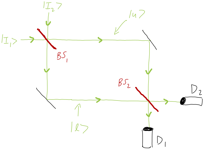
On the top left, we have two input states being mapped to states that propagate along the two arms of the interferometer, which I’ve labelled \ket{u} for upper and \ket{l} for lower. These two beams are then reflected and put back together at the second beam splitter, where they are read out at the two detectors D_1 and D_2. (If we want to be really pedantic, we should write operators for the mirrors too since they will typically change the phase of the light when reflecting it, but since there’s a mirror on each side there’s no relative phase introduced and we can ignore the mirrors.)
Note that so long as the length of the two paths, upper and lower, is kept exactly equal, then we can completely ignore the propagation of the beams through free space; we know that our particles will pick up a phase as they propagate, but this amounts to an overall global phase if the path lengths are the same. As a result, the final state \ket{\psi_f} can just be written in terms of the input state \ket{\psi_i} using the action of the two beam splitters alone:
\ket{\psi_f} = \hat{U}_{BS_2} \hat{U}_{BS_1} \ket{\psi_i}.
While it is true that the operator representing a beam splitter is unitary, it’s important to emphasize that it’s actually mapping us between two different Hilbert spaces, contrary to the usual behavior where a unitary just represents a transformation within a fixed Hilbert space. This is a consequence of the way that we’re simplifying the treatment here, by isolating a two-state description instead of using the full Hilbert space (which involves the position space of the particles passing through, along with any other quantum numbers they might carry if we want to be complete.)
To be specific, the first beam splitter {\rm BS}_1 maps the input ports \ket{I_1}, \ket{I_2} to the beams \ket{u}, \ket{l}: \left( \begin{array}{c} \ket{u} \\ \ket{l} \end{array}\right) = \left( \begin{array}{ccc} && \\ &\hat{U}_{BS_1}& \\ && \end{array} \right) \left( \begin{array}{c} \ket{I_1} \\ \ket{I_2} \end{array}\right), while the second beam splitter takes \ket{u} and \ket{l} as inputs and then maps them into the states at the two detectors \ket{D_1}, \ket{D_2}: \left( \begin{array}{c} \ket{D_1} \\ \ket{D_2} \end{array}\right) = \left( \begin{array}{ccc} && \\ &\hat{U}_{BS_2}& \\ && \end{array} \right) \left( \begin{array}{c} \ket{u} \\ \ket{l} \end{array}\right),
We could, if we wanted to, write all of what we’re doing here in a dimension-6 Hilbert space that includes all of the states at once: two inputs, two paths, two detectors. But due to the way the experimental setup is constructed, we would write exactly the same matrices that I’m writing currently, padded by lots of extra zeros. So I’ll keep the current notation which is more compact, at the price that we’ll need to pay careful attention to the context when we write a matrix out.
We can just as well describe all of this using our density-matrix formalism, and that will be more convenient when we want to add measurments into the mix. From the way the states transform above, we have for a pure input state the result for the final density matrix at the two detectors
\hat{\rho}_f = \hat{U}_{BS_2} \hat{U}_{BS_1} \hat{\rho}_i \hat{U}_{BS_1}^\dagger \hat{U}_{BS_2}^\dagger. We can combine the action of the pair of beam splitters into a single evolution operator, \hat{E}_0 \equiv \hat{U}_{BS_2} \hat{U}_{BS_1}, and then we have \hat{\rho}_f = \hat{E}_0 \hat{\rho}_i \hat{E}_0^\dagger.
If you do the algebra out, you’ll find that for the pictured initial input of pure \ket{I_1}, there is constructive interference at detector D_2 and destructive at D_1, so the probability of measuring at D_2 is 1. In terms of density matrices, for the empty interferometer, \hat{\rho}_i = \left( \begin{array}{cc} 1 & 0 \\ 0 & 0 \end{array} \right) = \ket{I_1} \bra{I_1} \rightarrow \hat{\rho}_f = \left( \begin{array}{cc} 0 & 0 \\ 0 & 1 \end{array} \right) = \ket{D_2} \bra{D_2}.
So far, there is not much happening in our empty interferometer, but that’s precisely by design! We now have a setup to describe more interesting effects by introducing a difference between the two propagation paths that we can probe; and what could be more dramatic than adding a bomb?
17.5.2 The Elitzur-Vaidman bomb tester
Now we introduce a new element into our interferometer. We add a bomb to the upper arm, which is photosensitive - that is, it is triggered by detecting light. The bomb is perfectly sensitive to even a single photon passing by it, with 100% chance of detecting its presence if it is on the upper path. To match the original Elitzur-Vaidman setup, we will also assume that the bomb absorbs the photon when it is detected, so that regardless of how destructive the bomb is, no photon will be detected at the outputs if the bomb goes off.
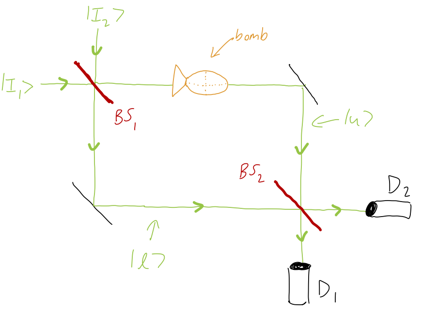
In the case where the bomb detonates, we have a projective (and dramatic) measurement that localizes the photon’s position, \hat{P}_{u} = \ket{u}\bra{u} = \left( \begin{array}{cc} 1 & 0 \\ 0 & 0 \end{array} \right) where the matrix form is in terms of the \ket{u}, \ket{l} basis and should be inserted at the appropriate place in our description. If we fire a photon through the apparatus and it doesn’t explode, then this gives the complementary measurement outcome \hat{P}_l = 1 - \hat{P}_u.
What does the presence of the bomb do to the output measurements of the interferometer? If we just select the case where the bomb doesn’t explode, then we insert the measurement projector in between the two beam splitters for the evolution. The probability of this outcome is p({\rm no\ boom}) = {\rm Tr} (\hat{\rho} \hat{P}_l) = {\rm Tr} (\hat{U}_{BS_1} \hat{\rho}_i \hat{U}_{BS_1}^\dagger \hat{P}_l) = \frac{1}{2} as we might have guessed. Note that in particular, this is the density matrix for the state traversing the interferometer, with one beam splitter applied. Now if we define the overall evolution operator as \hat{E}_l \equiv \sqrt{2} \hat{U}_{BS_2} \hat{P}_l \hat{U}_{BS_1}, (where 2 = 1 / p({\rm no\ boom}) fixes the normalization of the measurement) then for the same input purely through \ket{I_1} as pictured, we find \hat{\rho}_f = \hat{E}_l \hat{\rho}_i \hat{E}_l^\dagger = \frac{1}{2} \left( \begin{array}{cc} 1 & i \\ -i & 1 \end{array} \right).
The story so far is very simple: in the “empty” Mach-Zehnder interferometer, the interference of the two beam paths leads to 100% probability of detection at the second detector. When we add the bomb in, we force all detected photons to take the lower path \ket{l}, since we certainly can’t detect them if they follow \ket{u} and trigger the bomb. This removes the interference effect. From the final density matrix, we can read off that the probability of detection at either \ket{D_1} or \ket{D_2} is equal to the corresponding diagonal entry
These are all very simple observations, but we’ve actually revealed a very surprising effect. Let’s enumerate the possible outcomes and their probabilities:
- The bomb explodes (50%);
- We detect a photon in detector D_1 (25%);
- We detect a photon in detector D_2 (25%).
What is surprising about these outcomes? Suppose that the interferometer is in a black box and we don’t know if the bomb has been added to the upper path or not. If we send a photon in, 50% of the time we will quickly find out about the bomb (because the apparatus will explode), and 25% of the time we detect a photon at D_2, which is what would have happened if the bomb wasn’t there. But the last possibility is the most interesting: if we see the photon emerge at detector D_1, then we know for certain that there is a bomb in the interferometer - but we didn’t trigger the bomb to explode!
This is an interaction-free measurement: we avoided disturbing the state of the bomb, but were still able to gain information about it being present in the box. We can use this as a “bomb tester”, usefully. If we are working purely with classical physics, then we have to blow up every bomb that we test. But if we use a Mach-Zender interferometer as in the present setup, then from an initial population of 100 bombs, on average 50 of them explode, 25 of them may or may not be working, but 25 of them are certain to be working bombs that we haven’t blown up yet! (We can recover a few more than 25 of the bombs on average by running the ones we don’t know about through the test repeatedly until we know they work or until they blow up.)
Of course, the “bomb” description is very prosaic, but all of the math that we’ve done applies just as well to cases where the “bomb” is just a photomultiplier tube that absorbs and detects the photon on just the upper path. We arrive at the same surprising conclusion, that we can tell whether there is a working photomultiplier in the apparatus without ever looking at its output, and just by looking for the interference effect at the far end!
We could usefully reframe things a bit at this point, using some of the more fancy definitions we introduced above. In each of the two cases of our Mach-Zender interferometer with and without a live bomb present, we’ve written down an explicit mapping from initial to final density matrix, \hat{\rho}_i \rightarrow \hat{\rho}_f. This mapping is a quantum channel (since it preserves the properties of a density matrix), and the evolution operators \hat{E} that we’ve defined are in fact examples of Kraus operators, which we saw above in the context of time evolution. So if we want to describe the full range of outcomes, we can write a very similar expression to what we had above for time evolution, \hat{\rho}_f = \sum_\mu \hat{E}_\mu \hat{\rho}_i \hat{E}_\mu^\dagger where \mu = \{0, l\}. However, if we want to do this properly, we have to deal with the case that there is another “state” accessible to the system when the bomb explodes, which means we would have to expand our treatment to 3x3 density matrices (with the third entry always being zero in the case the bomb is inert.) Just for simplicity, I will keep the two-component notation for the rest of this discussion and just split out the different scenarios (in particular, bomb exploding vs. not) by hand; but in some ways, the treatment doing everything at once with a single (mixed) density matrix would certainly be cleaner.
17.5.3 Interaction-free measurement
Now that we have established that it’s possible to detect a bomb without disturbing it, a natural question is whether we can modify the experimental setup to improve the probability that we do so. The answer turns out to be emphatically yes, in fact the probability of measuring without interacting can be sent arbitrarily close to 1!
The basic idea actually takes us back to the quantum Zeno effect. We begin by modifying the initial beam splitter so that instead of producing a 50-50 split, it produces an arbitrary division depending on a mixing angle \theta: \hat{P}_{BS'}(\theta) = \left( \begin{array}{cc} \sin \theta & i \cos \theta \\ i \cos \theta & \sin \theta \end{array}\right) reproducing the 50-50 beam splitter we had before if we set \theta = \pi/4. For small \theta, the input beams will be mostly reflected, giving only a small transmitted component with amplitude proportional to \sin \theta. (This gives us a small chance of triggering the bomb, which is obviously desirable if we’re trying to save more of them.) We can propagate back through the apparatus to find that if we replace both beam splitters with BS’ (using the same angle \theta), the evolution operators are \hat{E}^{(\rm inert)} = \hat{U}_{BS'}(\theta)^2 \\ \hat{E}^{(\rm live)} = \frac{1}{\sqrt{p({\rm no\ boom})}} \hat{U}_{BS'}(\theta) \hat{P}_l \hat{U}_{BS'}(\theta) then the final density matrices are computed as above from \hat{\rho}_f = \hat{E} \hat{\rho}_i \hat{E}^\dagger, giving the results after a bit of algebra \hat{\rho}_f^{(\rm inert)} = \left( \begin{array}{cc} \cos^2 (2\theta) & -\tfrac{i}{2} \sin (4\theta) \\ \tfrac{i}{2} \sin (4\theta) & \sin^2 (2\theta) \end{array}\right) if the bomb is inert, and \hat{\rho}_f^{(\rm live)} = \left( \begin{array}{cc} \cos^2 \theta & i \cos \theta \sin \theta \\ -i \cos \theta \sin \theta & \sin^2 \theta \end{array} \right) if the bomb is live. The probability of the bomb surviving in the case where it is live is p({\rm no\ boom}) = {\rm Tr} (\hat{U}_{BS'}(\theta) \hat{\rho}_i \hat{U}_{BS'}(\theta) \hat{P}_l) = \cos^2 \theta.
(Setting \theta = \pi/4 recovers our previous case.) We can see the problem immediately: as we lower \theta, the probability of measuring the photon at D_1 is very high in both cases, so we get a very high false positive rate as a trade-off for reducing the probability of detonating the bomb. If we adjust \theta close to \pi/2, we have the opposite problem; the discrimination rate is very high, but the bomb will explode with a high probability as most of the incoming amplitude is transmitted along the \ket{u} path where the bomb is sitting.
But it turns out that we can improve our situation dramatically by doing the weak measurement, but doing it repeatedly. Instead of detecting the photon after one trip through the two arms of the M-Z interferometer, we send the two outputs from paths \ket{u} and \ket{l} back to the beginning of the interferometer and allow the photon to run through N times in total. This alters the final density matrices:, which now pick up N copies of the evolution operator: we now have \hat{\rho}_f = \hat{E}^{N/2} \hat{\rho}_i (\hat{E}^\dagger)^{N/2} (with the factor of 1/2 appearing because we’re chaining input to output, so each interferometer we add only adds one more beam splitter, not two.) To keep the small-angle and large-repetition limits tied together, and to maximize interference, we’ll fix the angle for each interferometer as \theta = \frac{\pi}{2N}.
Doing the algebra out again (and here it gets messy so I’ve just done things to leading order in Mathematica), we find first for the inert case \hat{\rho}_f^{(\rm inert)} \rightarrow \left( \begin{array}{cc} 0 & 0 \\ 0 & 1 \end{array} \right) for large N due to our selection of the total rotation angle as N (\tfrac{\pi}{2N}) = \pi/2. In other words, if the bomb is not present, the small transmitted amplitudes interfere repeatedly until we have a fully transmitted output at the other end of the interferometer, only in detector D_2.
On the other hand, if we deal with the live case carefully, we find precisely the opposite limit, \hat{\rho}_f^{(\rm live)} \rightarrow \left( \begin{array}{cc} 1 & 0 \\ 0 & 0 \end{array} \right). So we have perfect discrimination of whether the bomb is live or not! You might worry that the price we’ve paid is a high rate of exploding the bombs since we’re measuring many times, but we can work out the cumulative probability of an explosion happening in this measurement protocol: for each single interferometer the incoming probability of traversing the top path is always the same, so we simply have p({\rm no\ boom}) = \left(1 - \sin^2 \left( \frac{\pi}{2N} \right) \right)^N \\ \approx \left( \frac{\pi^2}{4N^2} \right)^N = \frac{\pi^2}{4N} As N goes to infinity, then, we have perfect results; we can test 100% of the bombs and we lose none of them. Although we’re measuring many times, the measurements are becoming weaker and weaker, and the scaling works out. In fact, we can think of what is happening here as a variation on the quantum Zeno effect; every time the bomb fails to explode, we are measuring the path taken by the photon and collapsing it to the pure state \ket{l}, slowing down the ordinary time evolution from \ket{l} to \ket{u} that happens slowly in the case where the bomb is not present and normal interference occurs. (If you read the Zeilinger paper, which I recommend because it’s very clearly written, this is exactly how it is presented!)