24 The helium atom
Now we’re ready to consider another example, a very important one: the helium atom. We will study helium first with perturbation theory, and then the variational method to compare. (We won’t do the example of Rayleigh-Ritz, but it yields the most precise results for helium energies and states.)
The helium atom has two orbital electrons, which we’ll label 1 and 2. Writing only the kinetic and Coulomb terms, the helium Hamiltonian is \hat{H} = \frac{\hat{p}_1^2}{2m} - \frac{Ze^2}{r_1} + \frac{\hat{p}_2^2}{2m} - \frac{Ze^2}{r_2} + \frac{e^2}{|\vec{r}_2 - \vec{r}_1|}. This is no longer a central potential, due to the repulsive force between the two electrons given by the last term. We can’t solve exactly, so we’ll treat the electron repulsion as a perturbation, writing the above as \hat{H} = \hat{H}_1 + \hat{H}_2 + \hat{W}.
With this choice, the unperturbed wavefunction can be decomposed into a product of two hydrogenic wavefunctions. However, we have to keep in mind that with two identical electrons, spin-statistics is active, which means that we must have either a symmetric or antisymmetric combination of wavefunctions, \psi_{\textrm{space}}^{(0)}(\vec{r}_1, \vec{r}_2) = \frac{1}{\sqrt{2}} \left[ \psi_{n_1,l_1,m_1}(\vec{r}_1) \psi_{n_2,l_2,m_2} (\vec{r}_2) \pm \psi_{n_1,l_1,m_1}(\vec{r}_2) \psi_{n_2,l_2,m_2}(\vec{r}_1) \right]. Which choice we make for a given state depends on the spin state of the electrons, which itself can also be symmetric or antisymmetric; we’ll see how this works in some specific examples. Before we consider spin, we can observe that with this setup the unperturbed energies for helium are just the sum of two hydrogenic energies: E_{n_1,n_2}^{(0)} = -Z^2 \left( \frac{1}{n_1^2} + \frac{1}{n_2^2} \right)\ \textrm{Ry} = (-54.4\ {\rm eV}) \left( \frac{1}{n_1^2} + \frac{1}{n_2^2} \right) plugging in Z=2 for helium. For the ground state n_1 = n_2 = 1, we find an energy which is 8 times the ground-state energy of hydrogen, or -108.8 eV.
It’s interesting to note that the ionization energy required to liberate one of the electrons is only half of the ground-state energy. The threshold for a free electron is at n=\infty, so we have for example E_{\infty,1}^{(0)} = -54.4\ {\rm eV}. This immediately implies that even the lowly n_1=2, n_2=2 energy level is unstable, since E_{2,2}^{(0)} = -54.4\ {\rm eV} \left( \frac{1}{4} + \frac{1}{4} \right) = -27.2\ {\rm eV}. This is well above the energy scale E_{\infty,1}^{(0)}. Because of this energy difference, the state \ket{2,2} will auto-ionize; there is a transition in which one electron goes to the ground state and the other escapes, leaving behind a {\rm He}^+ ion.
We will return to say more about auto-ionization later in these notes when we have better tools to describe the transition. For now, the key point to remember is that the stable states of an ordinary helium atom have at least one electron in the ground state. (This is all zeroth-order in perturbation theory, which isn’t quite right, but the qualitative conclusions and the existence of auto-ionizing states are robust.)
24.1 Helium ground-state energy: perturbative estimate
Let’s focus on just the ground state, where both electrons have n = 1. This forces the individual wavefunctions for both electrons to be in the \ket{nlm} = \ket{100} state, which in turn tells us that the spatial wavefunction must be symmetric, \psi_{g,\rm space}^{(0)}(\vec{r}_1, \vec{r}_2) = \psi_{100}(\vec{r}_1) \psi_{100} (\vec{r}_2) Fermi statistics then requires the overall wavefunction to be antisymmetric under exchange, which means that the spin wavefunction is definitely in the s=0 singlet state, \ket{\chi_g} = \frac{1}{\sqrt{2}} (\ket{\uparrow}_1 \ket{\downarrow}_2 - \ket{\downarrow}_1 \ket{\uparrow}_2).
Now let’s include the electron repulsion as a perturbation. We can evaluate the first-order energy correction for the ground state as an integral: E_0^{(1)} = \left\langle \frac{e^2}{|\vec{r}_1 - \vec{r}_2|} \right\rangle \\ = \int d^3 r_1 \int d^3r_2 \frac{|\psi_{100}(r_1)|^2 |\psi_{100}(r_2)|^2}{|\vec{r}_1 - \vec{r}_2|}. The hydrogenic ground-state wavefunction is, being careful to include the spherical harmonic to get the normalization right, \psi_{100}(r) = \frac{1}{\sqrt{\pi}} \sqrt{\frac{Z^3}{a_0^3}} e^{-Zr/a_0}. Dealing with the relative position of the electrons is trickier; we can rewrite |\vec{r}_1 - \vec{r}_2| = \sqrt{(\vec{r}_1 - \vec{r}_2)^2} \\ = \sqrt{r_1^2 + r_2^2 - 2r_1 r_2 \cos \theta}, where \theta is the relative angle between the two position vectors. Substituting in above, we have E_0^{(1)} = \left(\frac{Z^3}{\pi a_0^3} \right)^2 \int dr_1 r_1^2 e^{-2Zr_1 / a_0} \int dr_2 r_2^2 e^{-2Zr_2 / a_0} \\ \int d\Omega_1 \int d\Omega_2 \frac{e^2}{\sqrt{r_1^2 + r_2^2 - 2r_1 r_2 \cos \theta}}. We haven’t specified any coordinate axes yet; if we take the z axis to point along \vec{r}_1, then the angle \theta is just \theta_2, and we have E_0^{(1)} = \frac{8 Z^6 e^2}{a_0^6} \int dr_1 \int dr_2 (...) \int d(\cos \theta_2) \frac{1}{\sqrt{r_1^2 + r_2^2 - 2r_1 r_2 \cos \theta_2}}. The last remaining angular integral isn’t too bad: \int_{-1}^1 d(\cos \theta_2) \frac{1}{\sqrt{r_1^2 + r_2^2 - 2r_1 r_2 \cos \theta_2}} \\ = -\frac{1}{r_1 r_2} \left. \sqrt{r_1^2 + r_2^2 - 2r_1 r_2 \cos \theta_2}\right|_{-1}^1 \\ = -\frac{1}{r_1 r_2} (\sqrt{(r_1 - r_2)^2} - \sqrt{(r_1 + r_2)^2}) \\ = \frac{1}{r_1 r_2} (r_1 + r_2 - |r_1 - r_2|). Recognizing that the integral is totally symmetric under exchange of r_1 and r_2, we can assume r_1 > r_2 and just double the result; with this assumption, r_1 + r_2 - |r_1 - r_2| = 2r_2, so the above expression becomes simply 4 / r_1 (including the doubling due to symmetry.) Because we made this assumption, we also have to enforce it for the radial integrals by integrating r_1 over [r_2, \infty] instead of [0, \infty]. Doing a u-substitution first with u = Zr/a_0, we have
E_0^{(1)} = \frac{32 Ze^2}{a_0} \int_0^\infty du_2 \int_{u_2}^\infty du_1 u_1 u_2^2 e^{-2(u_1+u_2)}
The radial integrals are straightforward from here: they give a numerical factor of 5/256, so that we find for the energy correction E_0^{(1)} = \frac{5}{8} \frac{Ze^2}{a_0} = \frac{5Z}{4}\ \textrm{Ry}. This is a positive shift, changing the estimated ground-state energy for helium from -108.8 eV to -74.8 eV. This is a reasonably good estimate; the experimental value is around -78.98 eV.
24.2 Helium ground-state energy: variational estimate
Let’s see how the variational method does for helium, and whether we can gain any additional physical insight from that approach. There are many possible choices of variational wave functions, but a relatively simple approach turns out to work quite well. We’ll continue to assume that we can write the total wavefunction as a product of two hydrogenic wavefunctions, \tilde{\psi}(r) = \frac{1}{\sqrt{\pi}} \left( \frac{Z^\star}{a_0}\right)^{3/2} e^{-Z^\star r/a_0} and then \tilde{\psi}(r_1, r_2) = \tilde{\psi}(r_1) \tilde{\psi}(r_2). We take Z^\star to be our variational parameter; we could have tried a_0 as well, but since the wavefunction only depends on the ratio of the two the outcome would be the same. The trial energy is thus E(Z^\star) = \int d^3 r_1 \int d^3 r_2 \tilde{\psi}^\star(r_1) \tilde{\psi}^\star(r_2) \left( \frac{\hat{p}_1^2}{2m} - \frac{Ze^2}{r_1} \right. \\ \left. + \frac{\hat{p}_2^2}{2m} - \frac{Ze^2}{r_2} + \frac{e^2}{|\vec{r}_1 - \vec{r}_2|} \right) \tilde{\psi}(r_1) \tilde{\psi}(r_2). (note that this is the Hamiltonian so it is correct that the factors here contain Z and not Z^\star.) Rather than evaluating the integral directly this time, we can use some tricks. Notice that since the \tilde{\psi} function is just a ground-state hydrogenic wavefunction but with Z^\star as the atomic number, which means that \left( \frac{\hat{p}_1^2}{2m} - \frac{Z^\star e^2}{r_1} \right) \tilde{\psi}(r_1) = E_0(Z^\star) \tilde{\psi}(r_1) where E_0(Z^\star) = -(Z^\star)^2\ \textrm{Ry}, and similarly for r_2. In other words, \tilde{\psi}(r) is a ground-state eigenfunction of the “unphysical” hydrogen Hamiltonian with Z^\star. By rewriting -\frac{Ze^2}{r} = -\frac{Z^\star e^2}{r} + \frac{(Z^\star - Z) e^2}{r}, we reduce the big integral above to E(Z^\star) = 2 E_0(Z^\star) + 2(Z^\star - Z) e^2 \left\langle \frac{1}{r} \right\rangle_{Z^\star} + e^2 \left\langle \frac{1}{|\vec{r}_1 - \vec{r}_2|} \right\rangle_{Z^\star}. where the subscript Z^\star reminds us that we’re taking the expectation value with respect to the trial wavefunction. The first expectation value is just given by the virial theorem, e^2 \left\langle \frac{1}{r} \right\rangle_{Z^\star} = \frac{Z^\star e^2}{a_0} = 2Z^\star\ \textrm{Ry}. There’s no neat trick to evaluate the second expectation value, but we just found what it was in our perturbative estimate: e^2 \left\langle \frac{1}{|\vec{r}_1 - \vec{r}_2|} \right\rangle_{Z^\star} = \frac{5}{4} Z^\star\ \textrm{Ry}. Putting everything together, we see that E(Z^\star) = \left( 2(Z^\star)^2 - 4ZZ^\star + \frac{5}{4} Z^\star \right)\ \textrm{Ry}. This function is minimized for Z^\star_{\textrm{min}} = Z - \frac{5}{16}, giving the variational ground-state energy E(Z^\star_{\textrm{min}}) = - \left[ 2 \left(Z - \frac{5}{16} \right) \right]^2\ \textrm{Ry} \\ \approx -77.38\ \textrm{eV}. Comparing to the experimental value of -78.98 eV and our perturbative estimate of -74.8 eV, we see that the variational approach has given a significant improvement; and if we were more clever in our choice of variational function and parameters, we would be able to lower the variational bound and do even better. (As I mentioned, a Rayleigh-Ritz approach gives the best variational bounds on the helium ground-state and excited-state energies in practice.)
One other interesting point to make is that the result coming from our variational calculation has a sensible physical interpretation. We can think of Z^\star as an effective nuclear charge seen by each electron, which has been reduced by some amount due to “screening” by the presence of the other electron. The fact that this gives a very close answer to the true ground-state energy implies that this charge screening is the dominant correction to the non-interacting picture.
24.3 Spin-statistics and two electrons in an atomic orbital
To go beyond the ground state of helium, it’s important to understand that permutation symmetry requires us to exchange all of the quantum numbers on our two particles, not just a subset. This means that the requirement for (anti-)symmetry under permutation applies to the total wavefunction, and parts of it can have different properties. In particular, this means that we have to consider the combined spin state of our two electrons together with the combined orbital state. In general, we can split the overall wavefunction into spatial and spin parts, \psi(1,2) = \psi_{\textrm{space}}(1,2) \psi_{\textrm{spin}}(1,2). I’m writing the wavefunction as a completely generic function of labels 1 and 2, to remind ourselves that if we apply permutation it’s not just the position vectors \hat{\vec{r}}_1 and \hat{\vec{r}}_2 that we need to switch, but all of the \ket{nlm} quantum numbers. The key point is that only the total wavefunction must obey the spin-statistics theorem; even though we have two fermions, they can be in a symmetric spin state, as long as the spatial state is antisymmetric, or vice-versa.
What are the possibilities for the total spin wavefunction of the system? To consider total spin we have to add the two spin-1/2 angular momenta of the two electrons, which decomposes into s=0,1 as we’ve seen before: \ket{1,1} = \ket{\uparrow \uparrow} \\ \ket{1,0} = \frac{1}{\sqrt{2}} (\ket{\uparrow \downarrow} + \ket{\downarrow \uparrow}) \\ \ket{1,-1} = \ket{\downarrow \downarrow} \\ \ket{0,0} = \frac{1}{\sqrt{2}} (\ket{\uparrow \downarrow} - \ket{\downarrow \uparrow}). We’ve seen all this before, but it’s important enough to restate: the three “triplet” s=1 states are all symmetric under spin exchange, while the singlet s=0 state is antisymmetric.
It isn’t a coincidence that the permutation symmetry eigenvalue is determined completely by the total spin quantum number s; it’s easy to see why by construction. We can write the spin-lowering operator as \hat{S}_- = \hat{S}_{1-} + \hat{S}_{2-}. This is, clearly, invariant under permutation \hat{P}_{12}. That means that if we take the maximum-\hat{S}_z state \ket{s,s}, whatever its symmetry or antisymmetry properties are, all of the lowered states \ket{s,m_s} must have the same eigenvalue under permutation. In other words, we can check one state \ket{s,m_s} within each multiplet of fixed s to see if it’s symmetric or antisymmetric, and all other states with the same s will match.
Now let’s turn to the spatial part of the wavefunction. If the two electrons are in states \ket{nlm} and \ket{n'l'm'}, then the overall spatial wavefunction must take the form \psi_{\textrm{space}}(\vec{r}_1, \vec{r}_2) = \frac{1}{\sqrt{2}} \left[ \psi_{nlm}(\vec{r}_1) \psi_{n'l'm'} (\vec{r}_2) \pm \psi_{nlm}(\vec{r}_2) \psi_{n'l'm'}(\vec{r}_1) \right], with the sign between them being determined by the electron spin state:
- Total spin s=0 (singlet): the spin wavefunction is antisymmetric, which means that the spatial wavefunction is symmetric. The s=0 states are known collectively as para-helium states.
- Total spin s=1 (triplet): the spin wavefunction is symmetric, so the spatial wavefunction is antisymmetric. The s=1 states of helium are known as ortho-helium states.
In most cases, both ortho-helium and para-helium states are present. However, if we have two electrons in the same state, so n=n' and l=l', then we find some further restrictions. Most importantly, for the ground state \ket{100}\ket{100}, only the para-helium state exists; the would-be ortho-helium state has zero spatial wavefunction.
What about the general case \ket{nlm} \ket{nlm}? The answer now depends on what the total angular momentum of the combined two-electron state looks like. For example, suppose we have the state \ket{21m} \ket{21m}. Addition of two l=1 eigenstates gives the following possibilities for the \ket{L,M} combined state in terms of the individual \ket{l_1 m_1}_1 \ket{l_2 m_2}_2 states: \ket{2,2} = \ket{1,1}_1 \ket{1,1}_2 \\ \ket{1,1} = \frac{1}{\sqrt{2}} (\ket{1,1}_1 \ket{1,0}_2 - \ket{1,0}_1 \ket{1,1}_2) \\ \ket{0,0} = \frac{1}{\sqrt{6}} (\ket{1,-1}_1 \ket{1,1}_2 + \ket{1,1}_1 \ket{1,-1}_2 - 2 \ket{1,0}_1 \ket{1,0}_2) Here we can easily see that L=0,2 are totally symmetric under particle exchange, whereas L=1 is antisymmetric. It turns out that this is a very general observation that we’ve seen before: when combining two angular momenta, the Clebsch-Gordan coefficients obey the symmetry \left\langle j_1 j_2; jm | j_1 j_2; m_1 m_2 \right\rangle = (-1)^{j-j_1-j_2} \left\langle j_2 j_1; jm | j_2 j_1; m_2 m_1 \right\rangle. If we’re combining two equal l_1 = l_2 = l, then this immediately implies that for the total state, we simply have \hat{P}_{12} \ket{LM} = (-1)^{L} \ket{LM} matching the symmetry properties we see in the example above. So we see that in general, helium \ket{nlm}_1 \ket{nlm}_2 states where the total orbital angular momentum quantum number is L transform as (-1)^L under exchange.
So we see that there is an important relation between the spin state and the angular momentum state for helium when both electrons are in the same energy level. Since the spin-triplet (ortho) state is symmetric, it can only exist with angular momentum L=1. Likewise, the spin-singlet (para) state can only exist with angular momentum L=0 or L=2. Thus, we find missing energy levels, compared to what we would have expected for non-identical particles (or if the two electrons were in different orbitals.)
24.4 Exchange interaction and excited states of helium
There are some very important physical consequences of the sign in the spatial wavefunction that we’re now ready to explore. As we noted before, for a helium atom all stable bound states require one of the electrons to be in the n=1 orbital, or else the atom will have enough energy to auto-ionize. This means that the most interesting case to study is that where one electron is in state \ket{100}, and the other in a general state \ket{nlm}. The spatial part of the two-electron wavefunction can be written as \psi_{\textrm{space}}(\vec{r}_1, \vec{r}_2) = \frac{1}{\sqrt{2}} \left[ \psi_{100}(\vec{r}_1) \psi_{nlm} (\vec{r}_2) \pm \psi_{100}(\vec{r}_2) \psi_{nlm}(\vec{r}_1) \right].
Let’s have a look at the excited-state energies, once again treating the Coulomb repulsion between the electrons as a perturbation. For any choice of \ket{nlm}, we have for the unperturbed energy E^{(0)} = - Z^2 \left( 1 + \frac{1}{n^2} \right)\ \textrm{Ry}, and the energy correction is \Delta E = \left\langle \frac{e^2}{|\vec{r}_1 - \vec{r}_2|} \right\rangle. The spin part of the wavefunction has no effect on this perturbation, so the expectation value is taken purely with respect to the spatial part: \Delta E = \int d^3r_1 \int d^3r_2 |\psi_{\textrm{space}}(\vec{r}_1, \vec{r}_2)|^2 \frac{e^2}{|\vec{r}_1 - \vec{r}_2|}. If we expand out the spatial wavefunction, we find that we can write \Delta E = I \pm J, where I = \int d^3 r_1 \int d^3 r_2 |\psi_{100}(\vec{r}_1)|^2 |\psi_{nlm}(\vec{r}_2)|^2 \frac{e^2}{|\vec{r}_1 - \vec{r}_2|} is an integral of the form that we saw above for the ground state, and J = \textrm{Re} \left[ \int d^3 r_1 \int d^3 r_2 \psi_{100}^\star(\vec{r}_1) \psi_{nlm}^\star(\vec{r}_2) \frac{e^2}{|\vec{r}_1 - \vec{r}_2|} \psi_{100}(\vec{r}_2) \psi_{nlm}(\vec{r}_1) \right] is a new term, known as the exchange interaction (or “exchange energy.”)
In general, the value of J versus I will depend on what system we’re studying; it is even possible in some cases for J to be negative. For helium, it is the case that the para-helium states (singlet), which are spatially symmetric, have increased energy, while ortho-helium (triplet) states have lower energy. This makes physical sense, since we can think of the symmetrized spatial wavefunctions on average putting the electrons “closer” to each other, giving a larger energy contribution from the Coulomb repulsion between them, and vice-versa.
Since the difference between the two energies depends entirely on the spin state of the two electrons, it’s interesting to notice that we can actually rewrite the total energy shift in the form \Delta E = I - \frac{1}{2} \left(1 + \vec{\sigma}_1 \cdot \vec{\sigma}_2\right) J where as a reminder, the \sigma_i matrices are the dimensionless versions of the \vec{S}_i operators; we have \vec{\sigma}_1 \cdot \vec{\sigma}_2 = +1 for the S=1 triplet state, and -3 for the S=0 singlet. Thus, we find that even without any explicit spin dependence included in the Hamiltonian, the presence of Fermi-Dirac statistics here has induced a spin-dependent energy splitting - and a very large one, compared to the fine-structure spin effects we saw before! (This is purely electromagnetic and will be of order eV, not \alpha^2 times eV.) Despite being the same order, J is generally small compared to I, so we can think of it as giving us a splitting on top of the dual-hydrogen energy levels. Here is a quick sketch of the first few energy levels of helium:
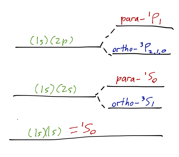
Here I’m using modified spectroscopic notation, {}^{2S+1}L_J, to label the energy levels. In hydrogen we always had 2s+1 = 2, so that label never changed; now for helium, the spin label is finally meaningful, distinguishing the para states (2s+1=1) from the ortho states (2s+1=3). For the set of states enumerated here, only ortho-(1s)(2p) helium has multiple J eigenvalues allowed, where \vec{J} couples total spin \vec{S} to total angular momentum \vec{L}.