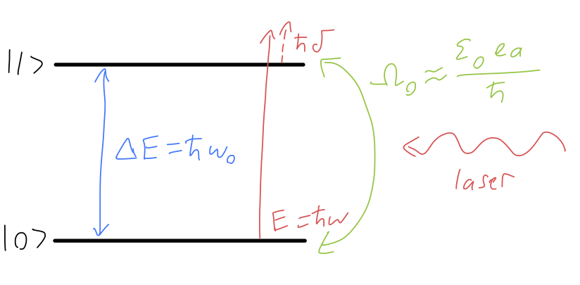
We now have enough math and physics under our belts to tackle a larger and more interesting piece of physics, known as Rabi oscillation. Our treatment of the two-state system so far, up to the “general solution” we wrote down, has been under the assumption of a constant Hamiltonian. But there are many interesting examples where the Hamiltonian becomes time-dependent, including broadly when we want to deal with light interacting with our quantum system, treating it as an oscillating electromagnetic wave. In most of quantum mechanics, dealing with time-dependence within the Hamiltonian itself becomes extremely complicated very quickly. But in the simplified confines of the two-state system, we can make a lot of progress.
5.1 Driving an atomic transition with a laser
To put things in physics context, let’s motivate the particular kind of time dependence we want to add to the Hamiltonian. Suppose we have a population of atoms for which we have isolated a single transition of interest, between two energy levels that we’ll label \ket{0} and \ket{1}, with E_0 < E_1 by assumption. These are both energy eigenstates of the unknown and probably complicated Hamiltonian \hat{H}_{\rm atom}, but if we restrict our attention to just these two states alone, then the system is equally well described by the much simpler Hamiltonian
\hat{H}_0 = \left( \begin{array}{cc} E_0 & 0 \\ 0 & E_1 \end{array}\right).
Since the energy splitting between the levels is of particular importance for time evolution, it’s often useful to rewrite this to expose it more explicitly as
\hat{H}_0 = \left( \begin{array}{cc} E_0 & 0 \\ 0 & E_0 + \hbar \omega_0 \end{array}\right)
where \omega_0 = (E_1 - E_0) / \hbar is the natural frequency associated with this transition. The time evolution in this system before we add anything else is trivially found using energy eigenstates: if we start in
\ket{\psi(0)} = \alpha \ket{0} + \beta \ket{1},
then the time-evolved state is, discarding the global phase which depends on E_0,
\ket{\psi(t)} = e^{-i\hat{H} t/\hbar} \ket{\psi(0)} = \alpha \ket{0} + e^{-i\omega_0 t} \beta \ket{1}.
Since the global phase isn’t physically meaningful, we see that only the energy splitting gives meaningful time evolution. (This is good, since as you’re used to from classical physics, the choice of zero-point for energy is not important for physics, only energy differences are.) In terms of energy levels, the probability of finding the system in either \ket{0} or \ket{1} is fixed in time; in particular, if our atom starts in either energy eigenstate, it will stay there forever. From this point forward, without losing any generality I’m just going to set E_0 = 0.
Now let’s make things more interesting by shining a laser on our atom. We can usefully assume the laser has a high enough intensity that we can ignore the quantization of light, and treat it as providing a background electromagnetic field. To describe a light wave, we need to know its amplitude, its frequency, and which way it is traveling. The last two are captured together by the wave vector \vec{k}, to which the oscillating \vec{E} and \vec{B} fields are transverse. The magnitude k \equiv |\vec{k}| is the wave number of the light, which is related to frequency as \omega = ck and wavelength as k = 2\pi / \lambda.
Instead of bothering to write out the full solution for a light wave, let’s just start with the simple observation that the size of an atom is, at the order-of-magnitude level, set by the Bohr radiusa_0 \approx 5 \times 10^{-11} m. On the other hand, the frequency of optical (visible) light is around 500 THz = 5 \times 10^{14} / s, or converting back to wavelength
\lambda = \frac{2\pi}{(\omega/c)} = \frac{c}{f} \approx \frac{3 \times 10^8\ {\rm m} / {\rm s}}{5 \times 10^{14}\ /{\rm s}} \approx 600\ {\rm nm}
which is four orders of magnitude larger than a_0. In other words, to very good approximation, the spatial structure of visible light is completely neglectable on the scale of a single atom; we can treat it as just a static background field oscillating in time. The field does have both electric and magnetic components, but the magnetic field has to couple to the motion of the orbital electron(s), and I’ll state another fact without proof that for e.g. a hydrogen atom, the electron has an average speed of v/c \sim \alpha \sim 1/137, so the magnetic field is also negligible to 1% accuracy or so. Thus, we can simplify our analysis greatly: the effect of the laser light on our system will be exactly just applying an oscillating electric field,
E(t) = \mathcal{E}_0 \cos \left( \omega t\right)
where \omega is the frequency of the laser light.
To proceed from here, our next step is to write out the Hamiltonian describing our atomic states, which requires figuring out how an orbital electron interacts with an applied electric field. This is something which we will cover in depth much later in these notes, and it would be too much of a detour to rehash the same ideas here. Instead, I’ll borrow a fact from the more careful treatment: A uniform electric field cannot couple an atomic orbital state to itself. The short explanation of this is that atomic orbitals, even the more complicated ones, are symmetric under reflection. Since the electric Hamiltonian is H_E = -q\vec{E} \cdot \vec{r}, the contributions from the points \vec{r} and -\vec{r} in the electron’s orbit cancel exactly.
The immediate consequence of this is that the electric field can only appear in the off-diagonal parts of our system Hamiltonian. This statement, plus the fact that the Hamiltonian must be Hermitian and the given time dependence above, is enough for us to write our modified Hamiltonian:
\hat{H} = \left( \begin{array}{cc} 0 & \hbar \Omega_0 \cos (\omega t) \\ \hbar \Omega_0 \cos (\omega t) & \hbar \omega_0 \end{array}\right).
(recalling that we got rid of the ground-state energy E_0 as a simplification.) We now have three frequencies in the problem:
The natural frequency, \omega_0 = \frac{E_1 - E_0}{\hbar};
The laser frequency, \omega;
The Rabi frequency, \Omega_0.
The Rabi frequency has some details swept into it: it is obviously proportional to the electric field strength \mathcal{E}_0, but it also depends on the properties of the atomic states themselves (specifically, a quantity known as the transition dipole matrix element which we’ll see how to compute explicitly much later.) Without trying to dig into the details, we can make a dimensional analysis estimate for the Rabi frequency. We have already established that \Omega_0 \propto \mathcal{E}_0; since this is a coupling to the orbital electron, it must also be proportional to the electron’s charge, so \Omega_0 \propto e. If we want to combine these to make an energy, we need a length scale, and the only one available is the size of the atom itself, which we’ll call a. Then,
\Omega_0 \approx \frac{\mathcal{E}_0 e a}{\hbar},
and we expect the atomic size a to be somewhere in the ballpark of the Bohr radius a_0, increasing somewhat as we go up the periodic table.
Before we proceed, it’s useful to think about how the three frequencies we’ve introduced might be related to one another. The laser frequency \omega is arbitrary, in the sense that it’s a parameter of the experiment that we choose to set up. However, something we haven’t talked about yet is the justification for our two-state model in what is surely a very complicated atom with hundreds of energy levels present. If we use a laser with an arbitrary frequency, we might be more likely to excite one of the other transitions that we’re ignoring. To justify only focusing on the chosen \ket{0} and \ket{1}, we need our laser light to basically couple only to that transition and none of the others. In practice, this means we need to tune closely to the natural frequency, that is, we must have \omega \approx \omega_0. Since this is assumed to be small, we can introduce a useful small parameter
\delta \equiv \omega - \omega_0
which is known as the detuning frequency. We’ll keep the smallness of this parameter in mind below.
In general, we can’t fully relate the Rabi frequency \Omega_0 to the other two, since it depends on a different experimental knob: E_0, which is controlled by the laser intensity. However, it will turn out that in realistic scenarios we typically have \Omega_0 \ll \omega. We will make use of this approximation below as well. Here’s a sketch of the overall system with the frequencies labelled before we move on:
Sketch of the two-state laser example.
5.2 Solving the semiclassical Rabi Hamiltonian
The Hamiltonian we have arrived at, or other slightly different forms of the same, is known as the semiclassical Rabi Hamiltonian. (I have added the qualifier “semiclassical” to cover the way we’re treating the laser light as a classical field; searching for “Rabi Hamiltonian” or “quantum Rabi Hamiltonian” will more likely turn up the alternative version that includes quantization of light into photons, although the structure is the same.)
We have seen a couple of different methods so far to deal with solving for two-state time dependence; here, with explicit time dependence in the Hamiltonian, the best approach will be to write down and solve a system of differential equations. Let’s define our solution to be
\ket{\psi(t)} \equiv \left( \begin{array}{c} c_0(t) \\ c_1(t) \end{array}\right).
Simply plugging in to the time-dependent Schrödinger equation, then, we have the coupled system
\begin{cases}
i\hbar \dot{c}_0 &= \hbar \Omega_0 \cos (\omega t) c_1, \\
i\hbar \dot{c}_1 &= \hbar \Omega_0 \cos(\omega t) c_0 + \hbar \omega_0 c_1.
\end{cases}
Working with complex exponentials is going to make our lives easier, so let’s split the cosine up:
\begin{cases}
2i \dot{c}_0 &= \Omega_0 (e^{i\omega t} + e^{-i\omega t}) c_1, \\
2i \dot{c}_1 &= \Omega_0 (e^{i\omega t} + e^{-i\omega t}) c_0 + 2 \omega_0 c_1.
\end{cases}
With constant coefficients, we would proceed by differentiating the second equation to replace c_0 with \dot{c}_0 and then substitute in to get a single-variable differential equation for c_1. In this case, the presence of the time-dependent coefficient prevents us from using that trick. Instead, let’s try the ansatz (physics jargon for “clever guess”) of a complex exponential solution. If we take
c_{i} = A_i e^{-i \lambda_i t},
(the minus sign in the exponent is deliberate, matching on to the minus sign from the Schrödinger equation for positive energy.) Then plugging back in gives the matrix system
\begin{cases}
2 \lambda_0 A_0 e^{-i\lambda_0 t} = \Omega_0 A_1 (e^{-i(\lambda_1 + \omega)t} + e^{-i(\lambda_1 - \omega)t}) \\
2 \lambda_1 A_1 e^{-i\lambda_1 t} = \Omega_0 A_0 (e^{-i(\lambda_0 + \omega)t} + e^{-i(\lambda_0 - \omega)t}) + 2\omega_0 A_1 e^{-i\lambda_1 t}
\end{cases}
or in matrix form, dividing through to collect some of the exponents together,
\left( \begin{array}{cc} 2\lambda_0 & -\Omega_0(e^{-i(\lambda_1 - \lambda_0 + \omega)t} + e^{-i(\lambda_1 - \lambda_0 - \omega)t}) \\ -\Omega_0 (e^{-i(\lambda_0 - \lambda_1 + \omega)t} + e^{-i(\lambda_0 - \lambda_1 - \omega)t}) & 2(\lambda_1 - \omega_0) \end{array}\right) \left( \begin{array}{c} A_0 \\ A_1 \end{array}\right) = 0.
Now, for the ansatz to work, this system of equations has to be solvable for any t, which means we need to kill both exponentials off at once:
\lambda_1 - \lambda_0 \pm \omega = 0
which is impossible to satisfy unless \omega = 0. Normally, this would be the point where we declare our ansatz didn’t work and go back to try something else. But let’s see what happens if we try to satisfy one of the two conditions anyway. If we choose
\lambda_1 = \lambda_0 + \omega,
then plugging back in gives
\left( \begin{array}{cc} 2\lambda_0 & -\Omega_0(e^{-2i\omega t} + 1) \\ -\Omega_0 (1 + e^{2i\omega t}) & 2(\lambda_0 + \omega - \omega_0) \end{array}\right) \left( \begin{array}{c} A_0 \\ A_1 \end{array}\right) = 0.
Now we can apply a famous trick, known as the rotating wave approximation (or “RWA” for short.) Let me just state the RWA first, and then justify it: the approximation we take is that the e^{2i\omega t} term is oscillating so fast that it will just average to zero and we can discard it, replacing
e^{\pm 2i\omega t} \rightarrow 0.
Why is this justifiable? If we look at what else is in our solution at this point, we see the Rabi frequency \Omega_0, which satisfies \Omega_0 \ll \omega, and the detuning frequency \delta, which definitely satisfies \delta \ll \omega. By dimensional analysis, the solution we haven’t yet finished finding has to oscillate at some combination of \Omega_0 and \delta, which means that oscillation at \omega will be extremely rapid compared to whatever we find. (We can check this condition at the end, to make sure our solution is at least self-consistent.)
CautionBeyond the rotating wave approximation
Although in many realistic situations the RWA is a good approximation, there may be cases if we’re working at high precision where we need to do a better job. We can view the approximation we have just made as a series expansion at leading (zeroth) order in \Omega_0 / \omega as \omega \rightarrow \infty. If we worked at the next highest order, which I won’t do in these notes, we would find what is known as the Bloch-Siegert shift; this amounts to finding corrections to the frequency of our solution that go as \Omega_0^2 / \omega and a rapidly-oscillating component with amplitude \Omega_0 / \omega.
While I won’t consider these corrections in these notes, I wanted to warn you about them and give you the name under which you can find more information if you’re in a situation where they may be important.
Applying the RWA to the matrix equation above, and then setting the determinant of the matrix to zero, the condition for a solution to exist is now
4\lambda_0 (\lambda_0 + \delta) - \Omega_0^2 = 0 \\
\Rightarrow \lambda_0 = \frac{1}{2} \left( -\delta \pm \sqrt{\delta^2 + \Omega_0^2} \right) \equiv \frac{-\delta \pm \Omega}{2},
where
\Omega \equiv \sqrt{\delta^2 + \Omega_0^2}
is known as the generalized Rabi frequency; in the limit of small detuning \delta, it is approximately just \Omega_0. We find as our general solution two terms oscillating at slightly different frequencies,
\begin{cases}
c_0(t) &= A_0 e^{i(\delta + \Omega)t/2} + B_0 e^{i(\delta - \Omega)t/2}, \\
c_1(t) &= A_1 e^{-i(\omega + \omega_0 + \Omega)t/2} + B_1 e^{-i(\omega + \omega_0 - \Omega)t/2},
\end{cases}
remembering to impose that \lambda_1 = \lambda_0 + \omega for the second solution.
5.2.1 Resonant behavior
To see more of the physics coming from our solution, let’s choose some initial conditions and finish solving. We’ll begin by just taking \ket{\psi(0)} = \ket{0}, i.e. our whole population starts in the atomic ground state. This means that at t=0 we have c_0 = 1, which imposes A_0 + B_0 = 1. We could try to plug this back in, but so far this is only half of the boundary condition (which is why the amplitude is only partly determined.) Our other boundary condition is that c_1 = 0.
We could try to write out the solution for c_1(t) as well, but a more clever approach is to use the differential equations we started with. In particular, we had \dot{c}_0 \propto c_1 as the first equation, which means that the other boundary condition is equivalent to just setting \dot{c}_0 = 0. Taking a derivative of our solution above gives
\dot{c}_0(t) = \frac{i (\delta + \Omega)}{2} A_0 e^{i(\delta + \Omega)t/2} + \frac{i (\delta - \Omega)}{2} B_0 e^{i(\delta - \Omega)t/2}
or at t=0,
0 = (\delta + \Omega) A_0 + (\delta - \Omega) B_0.
If we combine the two conditions, then, we have
0 = (\delta + \Omega) A_0 + (\delta - \Omega) (1-A_0) \\
= 2\Omega A_0 + (\delta - \Omega) \\
\Rightarrow A_0 = \frac{\Omega - \delta}{2\Omega}
and then B_0 = 1 - A_0 = (\Omega + \delta) / (2\Omega). Putting it all back together, we find
c_0(t) = e^{i\delta t/2} \left( \frac{\Omega - \delta}{2\Omega} e^{i\Omega t/2} + \frac{\Omega+\delta}{2\Omega} e^{-i\Omega t/2} \right) \\
= e^{i\delta t/2} \left( \cos \left( \frac{\Omega t}{2} \right) - \frac{i\delta}{\Omega} \sin \left( \frac{\Omega t}{2} \right) \right).
This is sufficient to talk about what is actually observable in this state, which is the probability. Squaring out, the time-dependent probability of observing the system in the ground state is
p_0(t) = |c_0(t)|^2 = \cos^2 \left( \frac{\Omega t}{2} \right) + \frac{\delta^2}{\Omega^2} \sin^2 \left( \frac{\Omega t}{2} \right) \\
= 1 - \frac{\Omega_0^2}{\Omega^2} \sin^2 \left( \frac{\Omega t}{2} \right),
and then p_1(t) = 1 - p_0(t) just picks off the second oscillating term,
p_1(t) = \frac{\Omega_0^2}{\Omega^2} \sin^2 \left( \frac{\Omega t}{2} \right).
which is known as Rabi’s formula. So the probability oscillates sinusoidally, but with a maximum amplitude given by
\frac{\Omega_0^2}{\Omega^2} = \frac{\Omega_0^2}{\Omega_0^2 + (\omega - \omega_0)^2}
This is an example of resonant behavior: the amplitude is peaked where the detuning vanishes, and dies off if the laser is moved away from the natural frequency. In the limit that \Omega_0 is large compared to the detuning, this is just close to 1; in the opposite limit, the amplitude dies off rapidly as the detuning increases. If we consider this as a function of the laser frequency \omega, it follows a Lorentzian distribution, whose width is given by \Omega_0. Since \Omega_0 itself was proportional to the field strength \mathcal{E}_0, we see that a more powerful laser will be more forgiving in terms of allowing oscillations to happen with some mistuning present.
Here is a plot showing the two probabilities oscillating together with our chosen initial condition of being purely in the ground state. The plot is given in units of the Rabi oscillation period T_0 = \Omega_0 / 2\pi. Notice that both the maximum value of P_1(t) and the period of oscillation (since \Omega > \Omega_0) are shifted by the presence of detuning.
Code
import matplotlib.pyplot as pltimport numpy as npdef p1(t, delta): Omega = np.sqrt(delta**2+ omega0**2)return (omega0**2/ Omega**2) * np.sin(Omega * t /2) **2omega0 =1.0# natural units: Rabi frequency Omega_0 = 1t = np.linspace(0, 4* np.pi, 400) # time in units of 1/Omega_0x = t / (2* np.pi)delta_fixed =0.30# still in units of Omega_0, so 30% mistuningp1_fixed = p1(t, delta_fixed)p0_fixed =1- p1_fixedfig2, ax = plt.subplots(figsize=(7, 4.5), dpi=150)ax.plot(x, p0_fixed, label=r"$P_0(t)$", color="#1f77b4", linestyle="-", linewidth=2)ax.plot(x, p1_fixed, label=r"$P_1(t)$", color="#d62728", linestyle="--", linewidth=2)ax.set_xlabel(r"$\Omega_0 t / 2\pi$")ax.set_ylabel("Probability")ax.set_xlim(0,2)ax.set_ylim(0, 1.05)ax.set_title(r"$\delta/\Omega_0 = 0.30$")ax.legend(loc="right", frameon=False)ax.grid(alpha=0.3)ax.spines["top"].set_visible(False)ax.spines["right"].set_visible(False)fig2.tight_layout()
Figure 5.1: Rabi oscillation probabilities P_0(t) and P_1(t) at a fixed detuning \delta/\Omega_0 = 0.30.
5.2.2 Revisiting the RWA in the rotating frame
We can find a bit more clarity with exactly how the rotating-wave approximation works - as well as another way to see how our solution works - by thinking a little differently about the time dependence of our state vector. At the very beginning of this chapter, we noted that even before we turn on the laser, there is some “free” evolution of the system, with a relative phase of e^{-i\omega_0 t} appearing between the two basis states. We can redefine our solution coefficients to absorb this phase away; doing so takes us closer to something like the interaction picture (which we’ll discuss in a later chapter.) Instead, let’s do something slightly different by putting the laser frequency into one of our coefficients:
\tilde{c}_0(t) \equiv c_0(t), \\
\tilde{c}_1(t) \equiv c_1(t) e^{i\omega t}.
(This is known as the “rotating frame”, specifically the “drive frame” since we’re using the frequency of the driving laser and not the natural frequency \omega_0, but they are equal up to the detuning.) If we go back and rewrite the Schrödinger equation in terms of these redefined coefficients, we see something interesting has happened:
\begin{cases}
i\hbar \dot{\tilde{c}}_0 = \hbar \Omega_0 \cos (\omega t) e^{-i\omega t} \tilde{c}_1, \\
i\hbar \dot{\tilde{c}}_1 = \hbar \Omega_0 \cos(\omega t) e^{i\omega t} \tilde{c}_0 - \hbar \delta \tilde{c}_1,
\end{cases}
using \dot{\tilde{c}}_1 = \dot{c}_1 e^{i\omega t} + i \omega \tilde{c}_1(t) on the second line. Now if we split this apart into components according to the oscillations at \omega and rewrite it in matrix form, we see that this takes the form of a “rotating-frame Hamiltonian”,
\hat{\tilde{H}} \equiv \frac{\hbar}{2} \left( \begin{array}{cc} 0 & \Omega_0 \\ \Omega_0 & -2\delta \end{array}\right) + \frac{\hbar}{2} \left( \begin{array}{cc} 0 & \Omega_0 e^{2i\omega t} \\ \Omega_0 e^{-2i\omega t} & 0 \end{array}\right).
In this set of variables, we have an exactly constant Hamiltonian (the first term), plus a “counter-rotating” part (the second term) which is oscillating at frequency 2\omega. This provides another way to apply RWA without making an ansatz first: we can discard the rapid oscillations already at the level of the Hamiltonian and then solve the simplified system.
TipMagnetic resonance
Another closely related Hamiltonian to the one we have been working with appears in the context of magnetic resonance. The setup is a bit more specialized than the general laser + atomic transition problem we have been solving so far. In this case, our two-state system is instead an electron in an applied external magnetic field. The magnetic field is taken to be time-dependent in a very particular way: we apply a large, constant component in the z direction, along with a small component that rotates around the xy plane with fixed angular frequency \omega:
\vec{B} = (b \cos \omega t, b \sin \omega t, B).
(We’ll just treat this as a magnetic field alone, but if you’re paying close attention you’ll recognize that if we ignore any spatial structure, this is the magnetic field for a circularly polarized light wave.) Recalling that the interaction of a spin with a magnetic field is given by \hat{H} \propto \hat{\vec{\sigma}} \cdot \vec{B}, we can write out the Hamiltonian in components as
\hat{H} = \frac{\hbar \omega_0}{2} \hat{\sigma}_z + \frac{\hbar \Omega_0}{2} \left( \hat{\sigma}_x \cos (\omega t) + \hat{\sigma}_y \sin (\omega t) \right) = \frac{\hbar}{2} \left( \begin{array}{cc} \omega_0 & \Omega_0 e^{-i\omega t} \\ \Omega_0 e^{i \omega t} & -\omega_0 \end{array} \right)
where we’ve now defined two angular frequencies
\omega_0 = \frac{eB}{m}, \\
\Omega_0 = \frac{eb}{m},
in close analogy to the same frequencies in the laser problem we’ve been solving. This is close to the same Hamiltonian we’ve been solving, but with the key difference that the off-diagonal components only have a single complex exponential instead of two. The result is that if we go to the rotating frame, there is no counter-rotating component: the Rabi solution is exact for magnetic resonance, with no need to apply the RWA. To be concrete, if we put our electron in the initial state \ket{\psi(0)} = \ket{\uparrow}, the probability of observing it flip to spin-down is
p(\downarrow) = \frac{\Omega_0^2}{\Omega^2} \sin^2 \left( \frac{\Omega t}{2} \right)
with \Omega \equiv \sqrt{\Omega_0^2 + (\omega - \omega_0)^2}. We see resonant behavior, but now with the difference that since there was no approximation made, we are free to adjust B and b freely, so we could have |b| \gg |B|. Nevertheless, the most interesting case is when |b| \ll |B|, which means that \Omega_0 \ll \omega_0. Then as a function of \omega, the transition probability becomes very sharply peaked (resonant) for \omega \approx \omega_0. This is the key idea behind methods like nuclear magnetic resonance (NMR) spectroscopy, which allows us to look for the response of a material to scanning the oscillation frequency \omega in order to measure \omega_0, or to do spatial imaging.
5.2.3 Quantum control
Now that we know the time dependence of our system, we can think about putting it to use. If we know the initial state of our system to good precision - for example, a pure ground state \ket{0}, which is often easy to prepare just by waiting for excited states to decay - then we can use our solution for time dependence to exert quantum control, converting our state into another state.
Given the Rabi oscillation solution, there are two obvious time values to consider. The first is
T_\pi \equiv \frac{\pi}{\Omega},
which when substituted in to the probability formulas gives
p_1(T_\pi) = \frac{\Omega_0^2}{\Omega^2}
which in the limit of perfect tuning \delta \rightarrow 0 becomes p_1(T_\pi) \rightarrow 1. A single pulse of laser light of duration T_\pi, applied on resonance with the natural frequency, is known as a \pi pulse; we can see that if done perfectly, it causes population inversion, with the ground state \ket{0} flipped to the excited state \ket{1} with 100% probability. If we tune \omega \neq \omega_0, then we lose some fraction of the probability; likewise if we set t not quite equal to T_\pi, it will cost us some of the probability as the sine oscillates slightly off of maximum. Both errors can be quantified, if we know the uncertainties on our experimental setup.
The other obviously interesting time value we can select for the system is
T_{\pi/2} \equiv \frac{\pi}{2\Omega}
which defines a \pi/2 pulse. Plugging this in gives \sin^2(...) = 1/2, so we find that in the limit of zero detuning, p_0(T_{\pi/2}) = p_1(T_{\pi/2}) = 1/2. This doesn’t completely pin down what state we get, however; there could still be a relative phase. (In Bloch sphere terms, we know the \pi/2 pulse is landing us somewhere on the equator, but we don’t know exactly where yet.)
The simplest way to see the effect of this pulse is actually to use the rotating-frame picture we hinted at above. In the limit of exact tuning, the rotating-frame Hamiltonian is just
\hat{\tilde{H}} \rightarrow \frac{\hbar \Omega_0}{2} \hat{\sigma}_x,
which we can just exponentiate to get the formal solution
\ket{\tilde{\psi}(t)} = \exp \left( -\frac{i\Omega_0 t}{2} \hat{\sigma}_x \right) \ket{\tilde{\psi}(0)} \\
= \left( \begin{array}{cc} \cos (\Omega_0 t/2) & -i \sin (\Omega_0 t/2) \\ -i \sin (\Omega_0 t/2) & \cos (\Omega_0 t/2) \end{array}\right)
using our matrix exponentiation results from the previous chapter. At the \pi/2 time specifically, and with \Omega = \Omega_0, this reduces to
\ket{\tilde{\psi}(T_{\pi/2})} = \frac{1}{\sqrt{2}} \left( \begin{array}{cc} 1 & -i \\ -i & 1 \end{array}\right) \ket{\tilde{\psi}(0)}.
So our initial state \ket{0} will be rotated into \frac{1}{\sqrt{2}} (\ket{0} - i\ket{1}) by a \pi/2 pulse, specifically. (This is in the rotating frame, so there’s an additional phase on the \ket{1} term, but it’s oscillating very rapidly as e^{i\omega_0 t}, so the “average phase” will be what we found here even when we go back to the lab frame.)
CautionQuantum control for quantum computing
We’ve covered a specific initial condition, but what is the effect of a \pi pulse more generally? Without going back and filling in all of the details, it should be clear from what we’ve found so far that if we start with the system in the purely excited state \ket{\psi(0)} = \ket{1}, then the formulas we found above for p_0(t) and p_1(t) are just swapped with each other. This means that a perfectly-tuned pi pulse will swap this initial state into the ground state with probability 1.
At this point, we can recognize that if the effect of the pi pulse is to swap our two basis states with each other, then it’s exactly a realization of the Pauli matrix \hat{\sigma}_x, or an “X gate” in the language of quantum computing,
\hat{U}(T_\pi) \approx \hat{X} = \left( \begin{array}{cc} 0 & 1 \\ 1 & 0 \end{array}\right),
where the approximately-equals-to sign reminds us that this is under the RWA and under perfect tuning. Still, up to these errors, we now see something very useful: a concrete way to implement a quantum computing operation. (More generally, as we saw from our study of the \pi/2 pulse, Rabi oscillations give us a way to implement an arbitrary x rotation as a quantum gate.)
Since we’re now close enough to real experiments to plug in some real numbers, let’s run through that exercise - which will give us a chance to see how well the RWA is holding in a real experiment as a nice byproduct. Since I invoked silver atoms as the prototype for the Stern-Gerlach experiments we’ve been leaning on, let’s stick with them: silver atoms have a strong infrared transition line with a wavelength of \lambda = 827 nm. This is in the right part of the light spectrum to be excited by a titanium-sapphire laser, which are pretty powerful; they can produce a total power of order 1 Watt.
To translate that into an electric field strength, we can go through the Poynting vector \vec{S}. Details can be found at this link, but the key result we need is that the electric field strength is, in SI units,
\mathcal{E}_0 \approx 27.5 \sqrt{S}\ {\rm V}/{\rm m}
where S is the Poynting vector magnitude in units of {\rm W}/{\rm m}^2. To estimate S, we take the power of the laser in W and divide by the focusing area in square meters. Let’s suppose we focus our Ti:sapphire laser with a spot size of 1 {\rm mm}^2: then S = 10^6\ {\rm W}/{\rm m}^2, and the field strength is \mathcal{E}_0 \approx 2.75 \times 10^4\ {\rm V}/{\rm m}. Now we plug in to our Rabi frequency estimate, using the rough size of a silver atom as a \approx 3a_0 \approx 1.5 \times 10^{-10}\ {\rm m},
\Omega_0 \approx \frac{\mathcal{E}_0 e a}{\hbar} = \frac{(2.75 \times 10^4\ {\rm V}/{\rm m}) (1.6 \times 10^{-19}\ {\rm C}) (1.5 \times 10^{-10}\ {\rm m})}{1 \times 10^{-34}\ {\rm J} \cdot {\rm s}} \approx 6.6 \times 10^9\ {\rm Hz}.
Given this frequency, the time to execute a \pi pulse is then T_\pi \approx 0.5 ns. This is pretty close to the speed of a classical processor, so if we’re thinking of quantum computing it seems like a feasible timescale to work with (ignoring all of the many complications that would arise if you wanted to do this for real, of course!)
Finally, let’s also check after the fact that the RWA is actually good here. Given the laser wavelength of 827 nm, the corresponding angular frequency is
\omega = \frac{2\pi c}{\lambda} \approx 2 \times 10^{15}\ {\rm Hz}
or 2 PHz; this is much, much faster than the timescale of the \pi pulse, so rotating-wave approximation seems like a very good description of this system.
5.2.4 Recap
To briefly review, we’ve now gone through three very different approaches to solving for time evolution in a quantum two-state system:
Energy eigenstate expansion (Larmor precession)
Operator algebra (coupling to an arbitrary magnetic field direction)
Differential equations (magnetic resonance)
I’ve deliberately shown all of these methods to you to emphasize that our “quantum toolkit” of problem-solving methods contains many approaches: we can often use more than one method for a given problem, but often selecting the right approach will make a given problem easier. (If you need practice, feel free to mix and match the approaches above with the problems and see what happens!)
Over the rest of the semester, we’ll be making use of all three approaches depending on the problem. Knowing which method to apply to a specific problem is an art - something you have to get a feel for by solving problems and seeing examples. This is, of course, not new in physics: in classical mechanics you already know that you can apply Newton’s laws, or conservation of energy, or the Lagrangian, or the Hamiltonian, and the best choice will vary by what system you’re studying and what question you’re asking.
If you’re used to quantum mechanics as wave mechanics, then two of these methods are familiar: the “time-dependent Schrödinger equation” is method 3, while the “time-independent Schrödinger equation” is method 1 (expansion in energy eigenstates.) It may take some time to build up your intuition in the more general case, especially for the operator method.