12 Translation symmetry
The specific examples of symmetries that we have seen thus far are discrete symmetries, meaning that they have a finite number of eigenvalues: for example, parity is either even or odd, but nothing else. More mathematically, the symmetry group of parity is \mathbb{Z}_2, which is a finite group. However, we live in a continuous world, and as a result many of the most interesting symmetries to work with are continuous symmetries: the most familiar ones from classical mechanics being translation (this chapter) and rotation.
As is usually the case, the study of symmetry will be very rewarding: among other useful gems, we will find a quantum version of Noether’s theorem, a deeper understanding of the canonical commutation relation, and some interesting physical constraints that arise in solid-state systems where only certain translations are symmetric.
12.1 Continuous symmetries
As we have seen in our examples so far, the operators which realize a symmetry transformation are (almost always) unitary, thanks to Wigner’s theorem. It is a general fact that if we have a Hermitian operator \hat{Q}, then we can construct a unitary operator by exponentiating it: \hat{U}(a) = \exp \left( -\frac{i \hat{Q} a}{\hbar} \right) (The sign and the presence of \hbar are by convention.) It should be clear that for Hermitian \hat{Q}, we have \hat{U}{}^\dagger \hat{U} = 1. In fact, what we’ve constructed here is a whole family of unitary operators, parameterized by the arbitrary constant a. The Hermitian operator \hat{Q} inside the exponent is called the generator of this family of unitary symmetry operators. We’ve seen an example of this construction before: the unitary time-translation operator, e^{-i\hat{H} t/\hbar}.
To explore this further, let’s define explicitly the translation operator which will act on our system by performing a finite shift; we’ll call it \hat{\tau}(L), to distinguish it from the more general \hat{T} transformation, and we consider the case of an arbitrary shift by some length scale L. The action on position states is obvious: \hat{\tau}(L) \ket{x} = \ket{x+L}. This tells us that the position operator itself must transform as \hat{\tau}^\dagger(L) \hat{x} \hat{\tau}(L) = \hat{x} + L. Furthermore, we expect that translation by -L and then by L should give back the original state, from which we see that \hat{\tau}^{-1}(L) = \hat{\tau}(-L). However, we can see that \hat{\tau}^\dagger(-L) \hat{x} \hat{\tau}(-L) = \hat{x} - L \\ \hat{\tau}^\dagger(L) [...] \hat{\tau}(L) = \hat{\tau}^\dagger(L) \hat{x} \hat{\tau}(L) - L \hat{\tau}^\dagger(L) \hat{\tau}(L) \\ = \hat{x} + L (1 - \hat{\tau}^\dagger(L) \hat{\tau}(L)) which, given the observation that \hat{\tau}^{-1}(L) = \hat{\tau}(-L), must equal \hat{x}; so we also find that \hat{\tau}(L) is a unitary operator (which Wigner’s theorem told us anyway, but it’s always good to check!)
This is clearly an example of a continuous symmetry, since it depends on a continuous parameter, the translation distance. Now let’s go back to our starting idea: can we write this in terms of another operator which is a Hermitian generator? To answer that question, it’s useful to study what happens when the translation becomes very small: \bra{x} \hat{\tau}(\epsilon) \ket{\psi} = \psi(x-\epsilon). We know that \epsilon = 0 corresponds to no translation at all, i.e. \hat{\tau}(0) = 1. Therefore, in the limit of small \epsilon we must be able to rewrite \hat{\tau}(\epsilon) by series expanding the exponential to find \hat{\tau}(\epsilon) = 1 - \frac{i\epsilon}{\hbar} \hat{G} + ... for some Hermitian generator \hat{G}. Expanding both sides of the above equation then gives us \left\langle x | \psi \right\rangle - \frac{i\epsilon}{\hbar} \bra{x} \hat{G} \ket{\psi} = \psi(x) - \epsilon \frac{d\psi}{dx}. So for spatial translations, \hat{G} is just the momentum operator, \hat{p}. Although we’ve only shown that momentum gives rise to infinitesmal translations, we can “build up” a finite translation operator as a series of many infinitesmal ones and this just gives us back the same exponential form, either directly from an infinite product: \hat{\tau}(L) = \lim_{N \rightarrow \infty} \left(1 - \frac{i \hat{p}}{\hbar} \frac{L}{N} \right)^N = \exp \left( -\frac{i \hat{p} L}{\hbar}\right), or just by writing the infinitesmal form as an exponential, and then \hat{\tau}(L) = \hat{\tau}(\epsilon)^N = \exp \left( \frac{-i \hat{p} \epsilon}{\hbar} \right)^N = \exp \left( \frac{-i \hat{p} (N \epsilon)}{\hbar} \right) \rightarrow \exp \left( \frac{-i\hat{p} L}{\hbar} \right).
So we know two generators: the Hamiltonian is the generator of time translations, and the momentum operator is the generator of spatial translations. As we already saw, for any symmetry, we may find that in addition to the states of our Hilbert space, some operators are left invariant as well, i.e. \bra{\psi} \hat{U}{}^\dagger \hat{A} \hat{U} \ket{\psi} = \bra{\psi} \hat{A} \ket{\psi}. Since \hat{U} is unitary, this is equivalent to the condition [\hat{A}, \hat{U}] = 0. Moreover, if \hat{U} is continuous, then we can write \hat{U} = 1 - i \hat{Q} (\Delta a) / \hbar + ..., and so this immediately implies that [\hat{A}, \hat{Q}] = 0. For symmetries of the Hamiltonian, this has a particularly important consequence; we find that if [\hat{H}, \hat{U}] = 0 and \hat{U} is a continuous symmetry generated by \hat{Q}, then [\hat{H}, \hat{Q}] = 0. This is really easy to derive, but important enough to put in a box:
If a continuous symmetry \hat{U} is a dynamical symmetry, i.e. if [\hat{U}, \hat{H}] = 0, then the corresponding generator \hat{Q} of \hat{U} is a conserved quantity, i.e. [\hat{U}, \hat{H}] = 0 \Rightarrow \frac{d\hat{Q}}{dt} = 0.
In classical mechanics, Noether’s theorem (symmetries lead to conserved quantities) should be familiar to you already; the quantum version is much simpler to derive, but no less powerful. So, from the examples we’ve seen, invariance of a physical system under translations in space and time lead to conservation of momentum and energy, respectively.
It is a fact that all known fundamental interactions do conserve energy and momentum; so as long as we take all of the interactions into account (so that we have no “external” sources or potentials), we will find that infinitesmal translation in time and space is always a symmetry.
Another connection back to our more general discussion: we noted that symmetries in physics generally have a corresponding symmetry-group structure. For a continuous symmetry, it’s easy to check (see the aside below) that the exponentiated generators \hat{U}(a) form a particular type of group known as a Lie group. Lie groups are infinite, and they are smoothly connected to the identity, meaning that infinitesmal transformations are well-defined (which, in turn, lets us naturally work with familiar tools like derivatives and power series.) The group GL(N,\mathbb{C}) that appeared in our definition of represenations is itself a Lie group.
The mathematics of Lie groups is deep and beautiful, but we won’t dive into the general story in this class, we’ll borrow important math results as we need them. As far as I know, all continuous symmetry groups in physics are Lie groups. Some of them have multiple parameters, like rotations in three dimensions, as we will see.
The exponential map that we use to write a unitary symmetry operator in terms of a Hermitian generator immediately implies some useful properties. If \hat{C}_a is a continuous symmetry operator with parameter a \in \mathbb{R}, and it is generated by \hat{C}_a = \exp \left( -\frac{i\hat{G} a}{\hbar} \right), then it satisfies the following properties:
Composition: \hat{C}_a \hat{C}_b = \hat{C}_{a+b}
Identity transformation: \hat{C}_0 = \hat{1}
Inverse + unitarity: \hat{C}_a^{-1} = \hat{C}_a^{\dagger} = \hat{C}_{-a}.
The last two properties tell us immediately that for infinitesmal parameter value \epsilon, \hat{C}_\epsilon = \hat{1} - i\epsilon \hat{G} / \hbar for Hermitian generator \hat{G}, so that \hat{C}_\epsilon \hat{C}_{-\epsilon} = \hat{1}
at first order in \epsilon. We can then derive the exponential map for arbitrary a, by repeatedly applying infinitesmal transformations or by using composition to derive a differential equation. (See Merzbacher 4.6.)
You will recognize these properties: they are exactly the properties of a group! Specifically, these relations (together with the exponential map from Hermitian generator to unitary operator) define an object known as a Lie group.
One final thing that is interesting to point out with our new formalism is that the connection between position and momentum through a symmetry operator gives us another way to understand the canonical commutation relation. Let’s consider a translation by an infinitesmal distance \epsilon: \hat{\tau}(\epsilon) \ket{x} = \ket{x+\epsilon} Now, if we apply \hat{x} to both sides, it should produce a factor of (x + \epsilon), since it’s the same state on both sides. But we can also calculate the commutator of \hat{x} with the translation operator: [\hat{x}, \hat{\tau}(\epsilon)] = [\hat{x}, \left(1 - \frac{i\hat{p} \epsilon}{\hbar} \right)] \\ = -\frac{i\epsilon}{\hbar} [\hat{x}, \hat{p}]. So this tells us that \hat{x} \hat{\tau}(\epsilon) \ket{x} = \hat{\tau}(\epsilon) \hat{x} \ket{x} + [\hat{x}, \hat{\tau}(\epsilon)] \ket{x} \\ (x+\epsilon) \ket{x+\epsilon} = x \ket{x + \epsilon} - \frac{i\epsilon}{\hbar} [\hat{x}, \hat{p}] \ket{x} \\ We can cancel off the x \ket{x+\epsilon} from both sides, and then notice that to leading order in \epsilon, \epsilon \ket{x+\epsilon} \approx \epsilon \ket{x}. Then comparing what we have left, we can see that for any state \ket{x}, \epsilon = -\frac{i\epsilon}{\hbar} [\hat{x}, \hat{p}] \\ \Rightarrow [\hat{x}, \hat{p}] = i\hbar. So now we don’t have to take the relation as a postulate; it’s something we can derive from the fact that momentum is the generator of translations!
One oddity in the derivation above is the statement that \ket{x} and \ket{x+\epsilon} are “approximately the same”. If you think about this for a moment, it seems confusing, since all of the position eigenstates are orthogonal. We can try to construct the difference between them more explicitly: \ket{x + \epsilon} = \ket{x} + \epsilon \ket{\phi} + \mathcal{O}(\epsilon^2) and then try to see what the state \ket{\phi} has to be. If we try to maintain orthonormality, we want it to be true that \left\langle x | x+\epsilon \right\rangle = 0. Expanding it out with our definition, \left\langle x | x+\epsilon \right\rangle = 0 = \left\langle x | x \right\rangle + \epsilon \left\langle x | \phi \right\rangle + \mathcal{O}(\epsilon^2). At first glance, this looks impossible, since the first term is 1 and the second term is order \epsilon, which is small. In fact, if we insist on an algebraic solution to this order, we see that we must have \ket{\phi} = \frac{1}{\epsilon} (\ket{x+\epsilon} - \ket{x}). This looks exactly like a derivative! In fact, this is what the “difference” state \phi has to be, since another way to derive it is to expand out the translation operator: \ket{x+\epsilon} = \hat{\tau}(\epsilon) \ket{x} \\ = \left(\hat{1} - \frac{i}{\hbar} \epsilon \hat{p} \right) \ket{x} + \mathcal{O}(\epsilon^2) \\ = \ket{x} - \frac{i}{\hbar} \epsilon \hat{p} \ket{x} + \mathcal{O}(\epsilon^2). So (with some extra constants) the difference between \ket{x} and \ket{x+\epsilon} is exactly the state \hat{p} \ket{x} - and we already know that the matrix elements of \hat{p} in position space look like the position derivative.
One last word on groups and representations. What is the symmetry group corresponding to translations? Well, since we can translate by any real number, it should be easy to convince yourself that translation is described by the group \mathbb{R}, the real numbers. \mathbb{R} is a Lie group, an especially simple one since all operations commute (we can apply two translations in either order and the result is the same.)
As for the representations, recall that for parity \hat{P}, we could decompose N-dimensional parity representations into one-dimensional representations (vectors) that were either even or odd under parity. Here, the mathematical result is similar; \mathbb{R} can be completely reduced to one-dimensional representations. Unlike parity, here there are an infinite number of such representations, and they are labelled by the momentum eigenvalue p (since each \ket{p} will transform slightly differently under \hat{U}(L).) In other words, the (irreducible) representations of translation symmetry are simply the momentum eigenvectors \ket{p}; to know how an arbitrary physical state transforms under translation, we just expand in momentum states (or position states, since we know that’s just a change of basis.)
12.2 Lattice translation symmetry
There is another, much more powerful example of a discrete symmetry that we can find in a potential V(x), which is known as periodicity: in one dimension, it is the condition that V(x \pm a) = V(x) for some particular length scale a. The corresponding symmetry transformation \hat{T} - shifting our potential by a finite length a - is known as finite translation or lattice translation (to distinguish it from symmetry under infinitesmal translations by some arbitrary \epsilon.) Obviously, this will be an extremely important symmetry for the description of crystals and other solid-state systems.
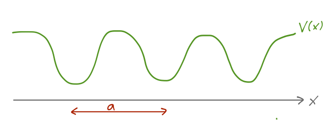
In this system, translation by an arbitrary length L will not be a symmetry. However, for the particular operator \hat{\tau}(a) such that \hat{\tau}^\dagger(a) V(\hat{x}) \hat{\tau}(a) = V(\hat{x} + a) = V(\hat{x}) then we find that \hat{\tau}^\dagger(a) \hat{H} \hat{\tau}(a) = \hat{H} \\ \Rightarrow [\hat{H}, \hat{\tau}(a)] = 0. where the last line follows since \hat{\tau}(L) is unitary. This commutator guarantees that we will be able to find simultaneous eigenstates of \hat{H} and \hat{\tau}(a).
12.2.1 Tight-binding approximation
It’s interesting to start with the case of a potential which is periodic, but with infinite potential barriers between neighboring identical wells of width a.
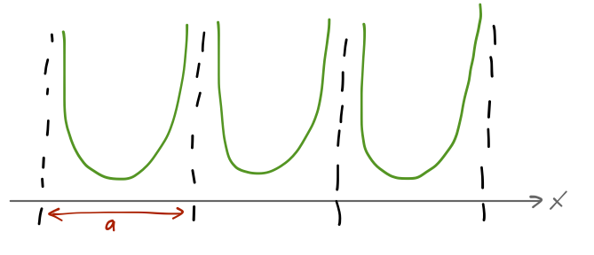
Suppose that if we solved the Schrödinger equation for one copy of this potential, we would find a set of bound states with energies E. Labeling the infinite set of wells by some integers n, we can construct a state \ket{n, E} which is equal to the E eigenstate in well n, and zero elsewhere. So \hat{H} \ket{n, E} = E \ket{n, E}, and there are an infinite number of such states in our infinite, periodic potential.
These states, however, are not eigenstates of the lattice translation operator, which clearly acts to give us \hat{\tau}(a) \ket{n, E} = \ket{n+1, E}. This should remind you a little bit of a ladder operator, and of coherent states in the simple harmonic oscillator, since it should be obvious that if we want to find an eigenstate of \hat{\tau}(a) it’s going to have to be in the form of an infinite sum. Let’s try a state of the following form: \ket{\theta, E} = \sum_{n=-\infty}^\infty e^{in\theta} \ket{n,E}. Acting with the translation operator, we see that \hat{\tau}(a) \ket{\theta, E} = \sum_{n=-\infty}^\infty e^{in \theta} \ket{n+1, E} \\ = \sum_{n=-\infty}^\infty e^{i(n-1)\theta} \ket{n, E} \\ = e^{-i\theta} \ket{\theta, E}. So indeed, \ket{\theta, E} is an eigenstate of lattice translation (and also of \hat{H}, since we constructed it as a sum of energy eigenstates.) The eigenvalue with respect to translation is a pure phase, so we can see that \ket{\theta, E} = \ket{\theta+2\pi, E} for any \theta. By convention we take the physical state to be labelled by -\pi < \theta \leq \pi.
Although the above derivation works just fine, the first step is a little vague. A reasonable question to ask is, why should the coefficients of \ket{\theta, E} be pure phases, instead of just arbitrary complex numbers?
The best way to answer this question is to just try the more general expansion: we allow an arbitrary complex coefficient for each well eigenstate,
\ket{T, E} = \sum_{n=-\infty}^\infty z_n \ket{n, E}.
Now what happens if we act with the translation operator? We find the following, doing the same sum redefinition trick: \hat{\tau}(a) \ket{T, E} = \sum_{n=-\infty}^\infty z_{n-1} \ket{n, E}. In general, there’s no reason for this state to be a translation eigenstate. But if we assume it is, then we find the equation \hat{\tau}(a) \ket{T, E} = T \ket{T, E} \\ \sum_{n=-\infty}^\infty z_{n-1} \ket{n,E} = T \sum_{n=-\infty}^\infty z_n \ket{n,E}. Since both sides are summing over the same states, every coefficient in the sum has to be identical, i.e. we find the result z_{n-1} = T z_n. This is a significant constraint, but it doesn’t prove the z_n must be a phase yet. We go a step further and apply the identity operator, in the form \hat{\tau}^\dagger(a) \hat{\tau}(a): \bra{T, E} \hat{\tau}^\dagger(a) \hat{\tau}(a) \ket{T,E} = |T|^2 since \bra{T,E} \hat{\tau}^\dagger(a) = (\hat{\tau}(a) \ket{T,E})^\dagger. But this is also just \left\langle T,E | T,E \right\rangle = 1, so T must be a pure phase T = e^{i\theta}, which means that z_n = e^{in\theta} z_0. So up to an overall constant, the form \ket{\theta, E} is the only possibility for an eigenstate of \hat{\tau}(a). The key here is actually a much more general result, which we basically just proved: the eigenvalues of a unitary operator are pure phases.
This is a good point to briefly connect back to our discussion about groups and representations. If we had a potential that was invariant under translation and was also finite, e.g. there was a periodic boundary somewhere (like a ring of N atoms), then we would have \hat{\tau}(a)^N = 1, and the symmetry corresponding to translation would be the cyclic group \mathbb{Z}_N. However, we’ve been considering the case of infinite potentials here, which we can think of as the limit of \mathbb{Z}_N with N \rightarrow \infty; this just gives us back \mathbb{Z}, the group formed by the integers under addition. Since \mathbb{Z} is infinite, a faithful representation in terms of our original basis \ket{n, E} takes the form of an infinite-dimensional matrix.
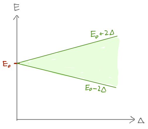
This is, so far, something of a formal exercise; the construction of the \ket{\theta, E} states doesn’t alter the energy spectrum at all since the wells have infinite barriers between them. At this point we’ll focus on a single eigenstate E_0, and label our well-centered states as \ket{n}. Let’s lower the barriers between the wells to be finite, but still high. In fact, we will assume that the barriers are high enough that while tunneling between adjacent wells is possible, leading to overlap of the wavefunctions, the overlap with wells separated by two or more barriers is totally negligible. In other words, the matrix elements of the Hamiltonian between localized states is \bra{n} \hat{H} \ket{n} = E_0 \\ \bra{n'} \hat{H} \ket{n} = -\Delta \delta_{n', n\pm 1}. This set of assumptions is known in solid state physics as the tight-binding approximation. Now, the localized states in an individual well are no longer energy eigenstates: the action of the Hamiltonian gives us \hat{H} \ket{n} = E_0 \ket{n} - \Delta \ket{n+1} - \Delta \ket{n-1}. However, it turns out that the \ket{\theta} translation eigenstates are still energy eigenstates! \hat{H} \ket{\theta} = E_0 \ket{\theta} - \Delta \sum_{n=-\infty}^\infty \left( e^{in\theta} \ket{n+1} + e^{in\theta} \ket{n-1} \right) \\ = E_0 \ket{\theta} - \Delta (e^{-i\theta} + e^{i\theta}) \ket{\theta} \\ = (E_0 - 2\Delta \cos \theta) \ket{\theta}. So as a result of the interaction term \Delta, our single, discrete bound-state energy has split into a continuous band of energies in the range E \in [E_0 - 2\Delta, E_0 + 2\Delta].
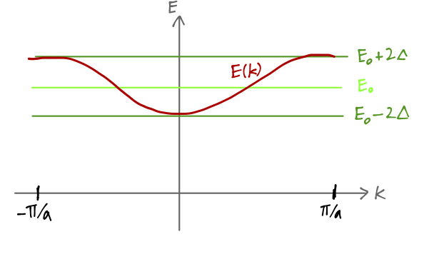
The wavefunctions corresponding to these continuous energies should also look different, now that tunneling between wells is allowed. We know that for any particular choice of \theta, the position-space wavefunction will be \left\langle x | \theta \right\rangle. But now we notice that \bra{x} \hat{\tau}(a) \ket{\theta} = \left\langle x-a | \theta \right\rangle \\ = \left\langle x | \theta \right\rangle e^{-i\theta} letting \hat{\tau}(a) act to the left and then to the right. For these two quantities to be equal, the wavefunction must be (1) periodic under lattice translation, except for (2) a part which kicks out exactly e^{-i\theta} when we shift x \rightarrow x-a. In other words, the wavefunction must take the form \left\langle x | \theta \right\rangle = e^{i\theta x/a} u_k(x), where u_k(x) is a periodic function with the same period as V(x), i.e. u_k(x+a) = u_k(x). The other piece here is a plane wave, from which we read off the wave number k = \theta/a. The observation above, that the wavefunction in the presence of a translation symmetry splits into a plane wave times a periodic function, is known as Bloch’s theorem; the periodic functions themselves are called Bloch functions. Preferring to work with the wave number, we see that the physical states are now labelled by -\pi/a < k \leq \pi/a, and the corresponding bound-state energies are E(k) = E_0 - 2\Delta \cos ka
This range of allowed distinct values for k is known as the Brillouin zone associated with this potential. The associated energy range E_0 - 2 \Delta \leq E \leq E_0 + 2\Delta is sometimes called the bandwidth.
It’s worth noting that the fact that we obtain a continuous band of energies E(k) is entirely because we have assumed that our potential is built from an infinite number of distinct, localized wells. We could have instead a finite chain of length N, say with periodic boundary conditions so that translation from well N returns us back to well 1. Then we must have \bra{x} \hat{\tau}(a)^N \ket{\theta} = \left\langle x | \theta \right\rangle = \left\langle x-Na | \theta \right\rangle = \left\langle x | \theta \right\rangle e^{iN\theta} which gives us a quantization condition, \theta = \frac{2\pi}{N} j where j is an integer between (-N/2, N/2). So with a finite number of states to translate between, we return to the case of having a discrete number of energy levels.
Let’s go back and focus more on the relationship between energy and wave number that we found above for the case when \ket{\theta} is also an energy eigenstate: E(k) = E_0 - 2\Delta \cos ka.
An equation of this form relating energy and wave number/momentum is known as a dispersion relation. What does this equation really mean, and why is it called a “dispersion relation”? The short answer is that the relationship between energy and wave number is crucial in how quantum states evolve in time and space. Recall that for a plane wave solution, the time-dependent wavefunction is u_E(x,t) = Ae^{i(kx-\omega t)} + Be^{-i(kx+\omega t)} where \omega = E/\hbar. A dispersion relation generalizes this form to systems where E(k) is different than the simple E \sim k^2 relationship for free particles. The exact form of the dispersion relation literally controls the dispersal of initial quantum states. (For example, a wave packet built of free plane waves will spread out in time. For a particle with linear dispersion, i.e. a photon \omega = ck, then there is no dispersal; the shape of a wave packet would be fixed as time evolves.)
12.3 Example: periodic delta functions
Let’s go back to periodic symmetry and try an explicit example with a simple model: a periodic array of identical delta functions, V(x) = \sum_{n=-\infty}^\infty V_0 \delta(x-na) where I’m assuming V_0 > 0.
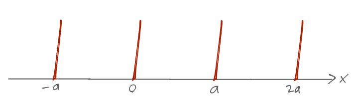
From our derivation before, we know that a general energy eigenstate can be written as a Bloch function times a plane wave, \psi(x) = e^{ikx} u_k(x) where u_k(x+a) = u_k(x). We also know that the full wavefunction between the delta functions must look like the sum of plane waves alone, \psi(x) = A e^{iqx} + B e^{-iqx}, where E(q) = \hbar^2 q^2 / (2m). Comparing the two equations, we see that the Bloch function has to be u_k(x) = A e^{i(q-k)x} + B e^{-i(q+k)x}. Now we apply the boundary conditions. Since u_k(0) = u_k(a), we see that A + B = A e^{i(q-k)a} + B e^{-i(q+k)a}. The other boundary condition, which you’re now quite familiar with from the homework, is that the derivative \psi'(x) will have a specific discontinuity due to the delta functions: \psi'(\epsilon) - \psi'(-\epsilon) = \frac{2mV_0}{\hbar^2} \psi(0) = \frac{2mV_0}{\hbar^2} (A+B). Exploiting the periodicity of the wavefunction, we can write \psi'(-\epsilon) = \psi'(a-\epsilon) e^{-ika}. Combining, we find the boundary condition \frac{2mV_0}{\hbar^2} (A+B) = iq[A (1-e^{i(q-k)a}) - B (1-e^{-i(q+k)a})]. Solving the two boundary conditions gives us a transcendental equation relating k and q: \cos (ka) = \cos (qa) + \frac{mV_0a}{\hbar^2} \frac{\sin(qa)}{qa}. (As a quick check on units: \hbar^2 has units of energy times time squared, [E]^2 [t]^2, which is [m]^2 [d]^2 / [t]^2. Dividing by ma leaves units of [m] [d] / [t]^2, mass times acceleration, which is energy - cancelling the V_0 so that the combination is dimensionless as it must be.)
Derive the equation above relating k to q, using the boundary condition equations we found above.
Answer:
Solving for continuity first, we can obtain the ratio B/A: 1 + \frac{B}{A} = e^{i(q-k)a} + \frac{B}{A} e^{-i(q+k)a} \\ \frac{B}{A} \left(1 - e^{-i(q+k)a} \right) = e^{i(q-k)a} - 1 \\ \frac{B}{A} = \frac{e^{i(q-k)a} - 1}{1 - e^{-i(q+k)a}}.
Now we plug this in to the other boundary equation: \frac{2mV_0}{\hbar^2} \left(1 + \frac{B}{A} \right) = iq [(1 - e^{i(q-k)a}) - \frac{B}{A} (1 - e^{-i(q+k)a})] \\ \frac{2mV_0}{\hbar^2} \frac{e^{i(q-k)a} - e^{-i(q+k)a}}{1 - e^{-i(q+k)a}} = iq[ (1 - e^{i(q-k)a}) - (e^{i(q-k)a} - 1)] \\ = 2iq(e^{i(q-k)a} - 1). This looks messy still, but let’s clear out the denominator on the left and try to simplify: \frac{mV_0}{\hbar^2} \left( e^{i(q-k)a} - e^{-i(q+k)a} \right) = iq(e^{i(q-k)a} - 1)(1 - e^{-i(q+k)a}) \\ \frac{mV_0}{\hbar^2} e^{-ika} (e^{iqa} - e^{-iqa}) = iq (e^{i(q-k)a} + e^{-i(q+k)a} - e^{-2ika} - 1) \\ \frac{mV_0}{\hbar^2} (2i \sin (qa)) = iq (e^{iqa} + e^{-iqa} - e^{-ika} - e^{+ika}) \\ = iq (2 \cos (qa) - 2 \cos(ka)) or cancelling off the 2i and rearranging, \cos(ka) = \cos(qa) + \frac{mV_0}{\hbar^2} \frac{\sin (qa)}{q} reproducing the result above.
Now we recall that q determines the energy of our state, E = \hbar^2 q^2 / 2m. In the limit q \rightarrow \infty, we just have \cos (ka) = \cos (qa), and we recover the standard free-particle dispersion E(k) = \hbar^2 k^2 / 2m. However, for smaller values of qa, the right-hand side of this equation can be larger than 1 (or smaller than -1), whereas the left-hand side can’t be.
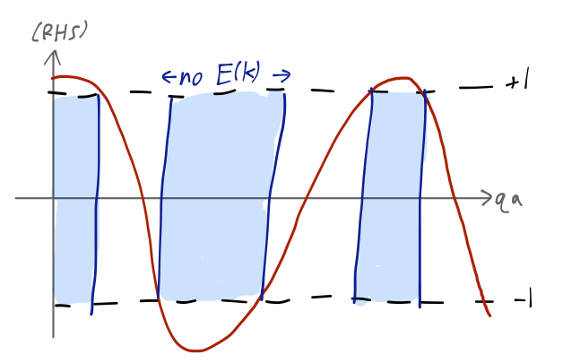
So certain values of E (and thus q) can never satisfy this equation. When the right-hand side of this equation is between -1 and 1, we find a continuum E(k) of possible energies, known as a band. The forbidden regions between the bands are known as band gaps.

Some bands have much larger separations in energy than others. If you imagine the bands as being filled with single electrons, you can begin to see the difference between a metal (in which it’s easy to excite an electron out of the ground state), and an insulator (in which it isn’t easy.)